1. Introduction
Modern photonic imaging systems, used in astronomy and in other areas of science, are required to perform with high imaging quality, a wide aperture (i.e., low F-numbers), and high spatial resolution. These systems are known as UWFOV systems. The wide-angle optical elements used in UWFOV systems introduce a significant shift variance [
1], which complicates the modeling task. Many recent research works have focused on finding a model of UWFOV systems that is suitable for reducing the uncertainties in reconstructing image data from wide-field microscopic systems [
2,
3,
4], security cameras [
5,
6,
7], and all-sky cameras [
8,
9,
10,
11,
12,
13,
14,
15]. Any imaging system can be described by its spatial impulse response function, commonly referred to as the Point Spread Function (PSF). PSF is used to represent the aberrations of UWFOV devices, and can be applied either to the entire image or within regions uniquely defined by the isoplanatic angle. However, it can sometimes be complicated to obtain a PSF model of the system. It can be difficult to achieve the desired accuracy using conventional methods—not from the measurement point of view, but because it is difficult to describe the space variance (SV) of the PSF over the Field of View (FOV). This leads to an obvious issue. From the measurement point of view, it is necessary to obtain the PSF for all discrete points of the entire FOV. Then the PSF of the system is described by such a field of individual PSFs. Born [
16] calls this type of PSF partially space-invariant because there are just discrete points (PSFs) in parts of the FOV. However, a space-variant PSF is described by a model in all points of the acquired image. Of course, this brings high demands on the precision of the model. Issues associated with sampling, pixel size and the pixel sensitivity profile must be taken into account in the design. It is very difficult to obtain the parameters of the model, especially in image areas with an aberrated impulse response and for objects with a small Full Width at Half Maximum (FWHM) parameter in relation to the pixel size. These objects, captured, e.g., in microscopy using all-sky cameras and/or special optical elements, can hardly be processed using current techniques, which are typically oriented to multimedia content.
A widely-used approach for obtaining the PSF is to model wavefront aberrations using Zernike polynomials. These polynomials were introduced by Zernike in [
17]. This work was later used by Noll [
18], who introduced his approach to indexing, which is widely used in the design of optics. Zernike polynomials are usually applied to rotationally symmetric optical surfaces. Zernike polynomials form a basis in optics with Hopkins [
19] field dependent wave aberration. Recently, Sasián [
20] reformulated the work of Hopkins. This new formulation is more practical for optical design. A more recent contribution by Ye et al. [
21] uses Bi-Zernike polynomials, which is an alternative to the method mentioned in Gray’s article [
22].
Zernike polynomials are used in modern interferometers for describing wave aberrations. However, researchers have begun to think about using these polynomials for an overall description of lens optics. When the first all-sky camera projects appeared, the question of how to model aberrations of fisheye lenses arose. Weddell [
23] proposed the approach of a partially space-invariant model of PSF based on Zernike polynomials. Another all sky project, Pi of the Sky [
1], focusing on gamma ray bursts, attempted to make a model of PSF. Their approach was quite different from Weddell’s [
23]. First, they calculate the dependency of the coefficients of the polynomials on the angle to the optical axis for several points. Then they interpolate these coefficients over the entire FOV. The WILLIAM project [
24] (WIde-field aLL-sky Image Analyzing Monitoring system) faces the issue of aberrations at an extremely wide-field FOV (see also [
25,
26]). Gray [
22] proposed a method for describing the spatial variance of Zernike polynomials. This approach is derived from the description provided by Hopkins [
19], and laid the foundations for truly space-variant Zernike polynomials. Of course, there is also the problem of space-variant PSF. In fact, we cannot be limited to rotationally symmetric imaging systems only. Hasan [
27] and Thompson [
28] came up with a more general description of the pupil function for elliptical or rotationally non-symmetrical Zernike polynomials. This description can be used for calculating the wave aberration in optical materials such as calomel for acousto-optical elements [
29]. The first optical approach to wave aberration estimation was described by Páta et al. [
30].
The search for the best description of UWFOV systems is not limited to astronomical imaging. Microscopy is another area where the UWFOV type of lens is used. Measurements of the special spherical aberration using a shearing interferometer were described in [
31]. A promising new approach was formulated in [
32]. It is based on aberration measurements of photolithographic lenses with the use of hybrid diffractive photomasks. The aperture exit wavefront deformation is modeled in [
33] for wide field-of-view fluorescence image deconvolution with aberration-estimation from Fourier ptychography.
UWFOV cameras are also used in surveillance systems. However, an image affected by aberrations can have a negative effect in criminal investigations [
6]. Ito et al. [
5] face this issue, and they propose an approach that estimates a matrix of coefficients of the wavefront aberrations. Many authors have reported on investigations of space-variant imaging systems. An estimate of the PSF field dependency is critical for restoring the degraded image. Qi and Cheng proposed their linear space-variant model [
34] and focused on the restoration algorithm for imaging systems. Heide et al. [
35] proposed techniques for removing aberration artifacts using blind deconvolution for the imaging system with a simple lens.
In our work, we propose a modeling method for PSF estimation for space-variant systems. Since we would like to use this model for general optical systems, the method is based on modeling the PSF of the system without knowledge of the wavefront. Thus, the method can be an alternative to the Shack–Hartmann interferometer [
4,
36], or to other direct wavefront measurement methods, since we can estimate wavefront aberrations from fitting PSF in the image plane. The following section begins with a description of wavefront aberrations.
2. Wavefront Aberration Functions
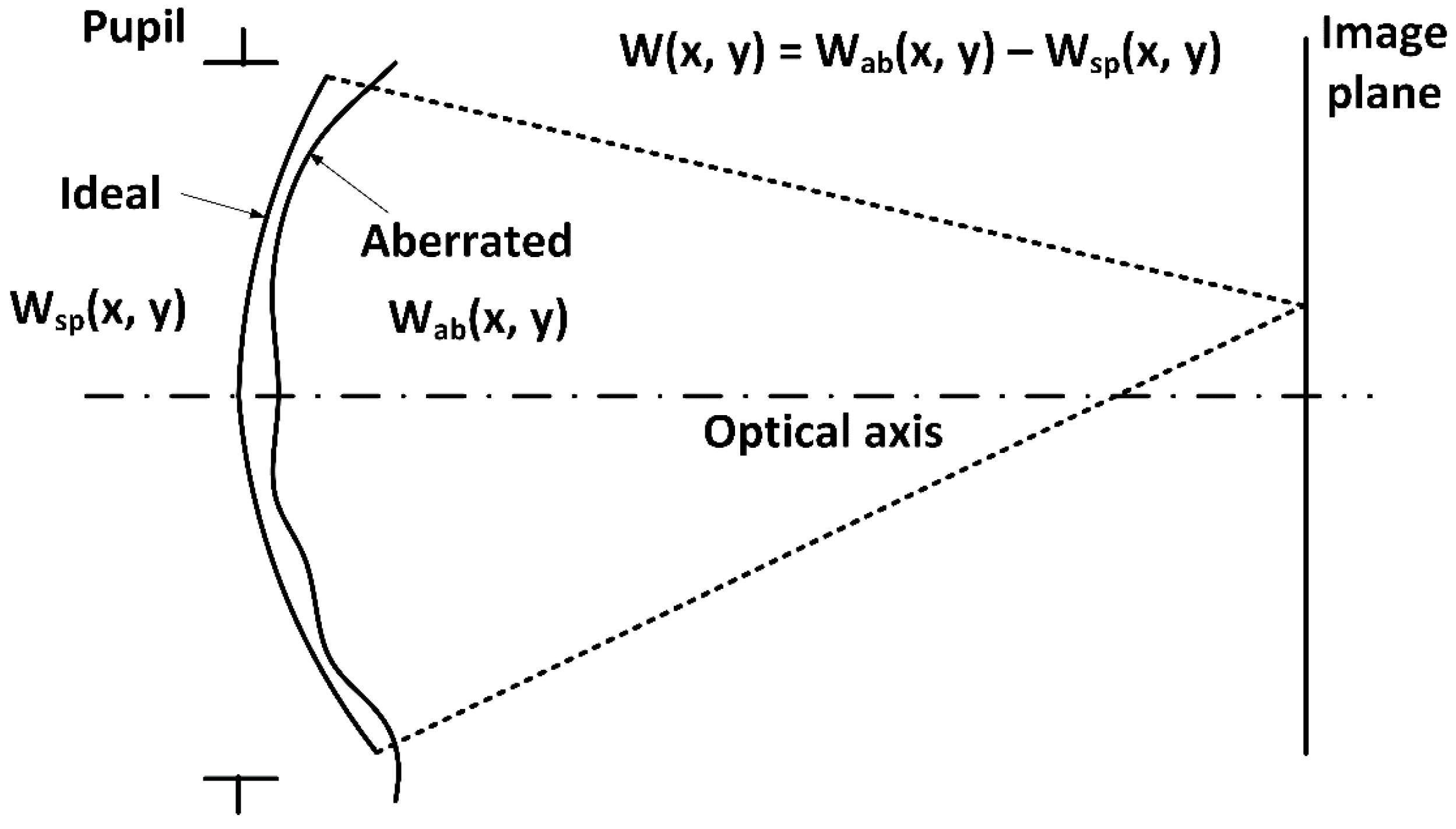
An ideal diffraction limited imaging system transforms a spherical input wave with an inclination equal to the plane wave direction. As described by Hopkins [
19], real imaging systems convert the input plane wave into a deformed wavefront. The difference between an ideal wavefront and an aberrated wavefront in the exit aperture can be expressed as
where
W(
x,
y) are wavefronts—the surface of points characterized by the same phase.
Figure 1 illustrates the shape of the ideal spherical wavefront
and aberrated wavefront
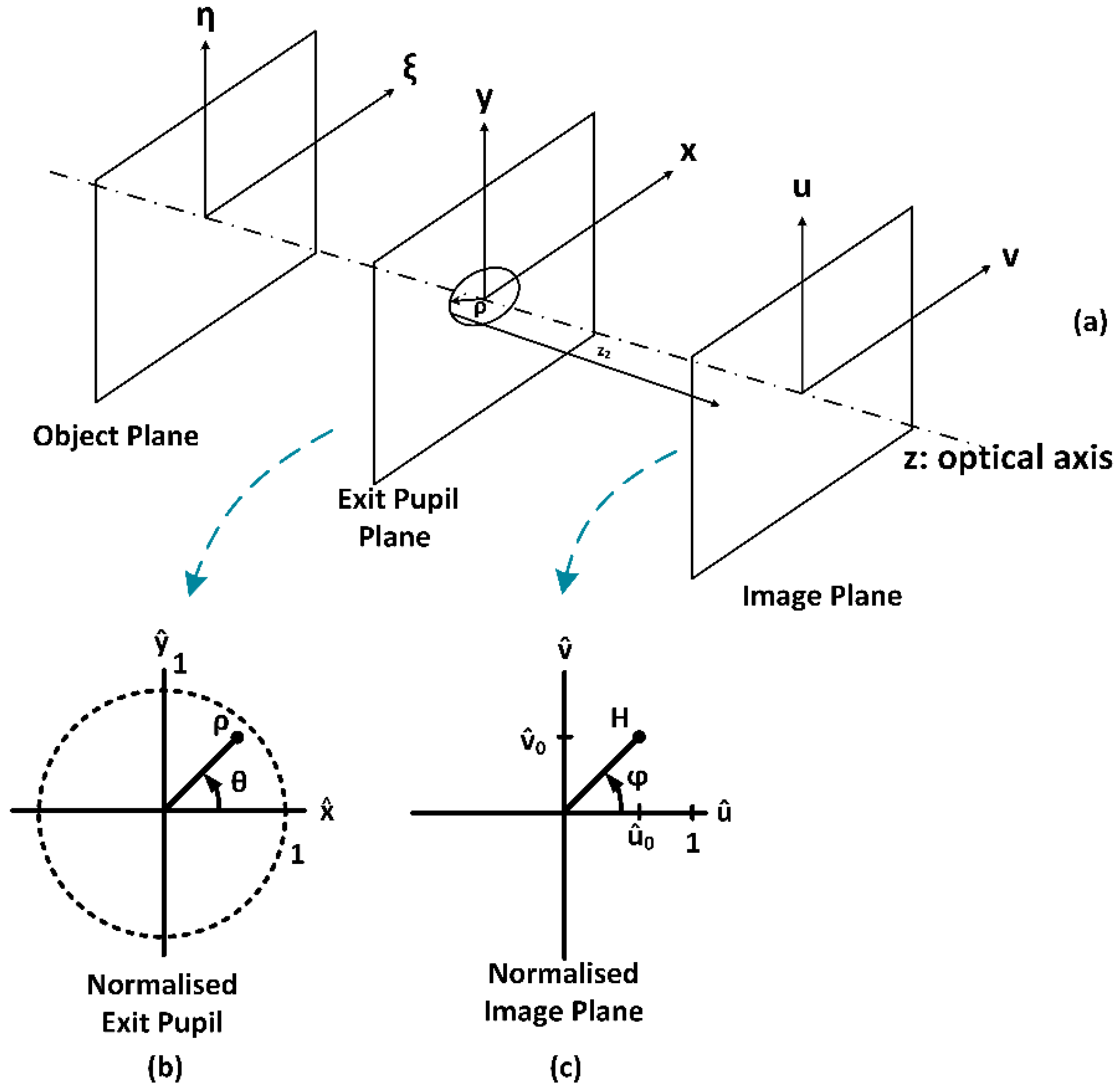
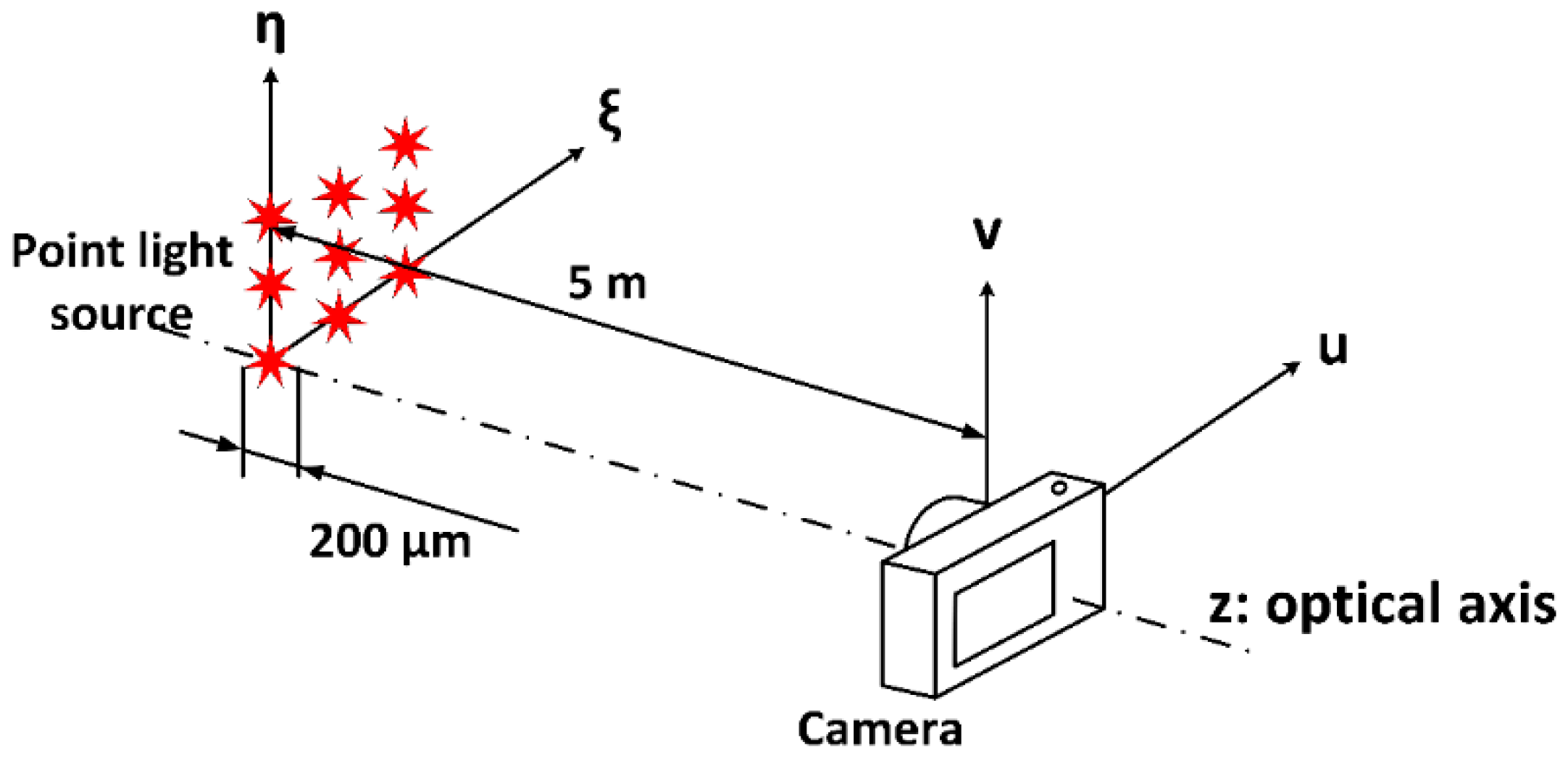
. It can be useful to introduce the coordinate system illustrated in
Figure 2. The object plane is described by the
ξ,
η coordinates; the exit pupil uses
x,
y notation, and the image plane uses
u,
ν notation. Then we introduce the
normalized coordinates (see
Figure 2b,c) at the exit pupil and ρ, θ polar coordinates. The normalized image plane coordinates are
and
H, ϕ, respectively.
The aberrated wavefront can be represented by a set of orthonormal base functions, known as Zernike polynomials. Zernike polynomials, which are described in [
17] and in [
37,
38,
39,
40], are a set of functions orthogonal over the unit circle, usually described in polar coordinates as
, where
ρ is the radius and
θ is the angle with respect to the
-axis in the exit aperture (see
Figure 2b). They represent functions of optical distortions that classify each aberration using a set of polynomials. The set of Zernike polynomials is defined in [
17]; other adoptions are in [
37,
38,
39,
40], and it can be written as
with
n describing the power of the radial polynomial and
m describing the angular frequency.
is the normalization factor with the Kronecker delta function
= 1 for
m = 0, and
= 0 for
m ≠ 0, and
is the radial part of the Zernike polynomial.
Any wavefront phase distortion over a circular aperture of unit radius can be expanded as a sum of the Zernike polynomials as
which can be rewritten using Equation (2) as
where
m has values of
k is the order of the polynomial expansion, and
is the coefficient of the
mode in the expansion, i.e., it is equal to the root mean square (RMS) phase difference for that mode. The wavefront aberration function across the field of view of the optical system can then be described as
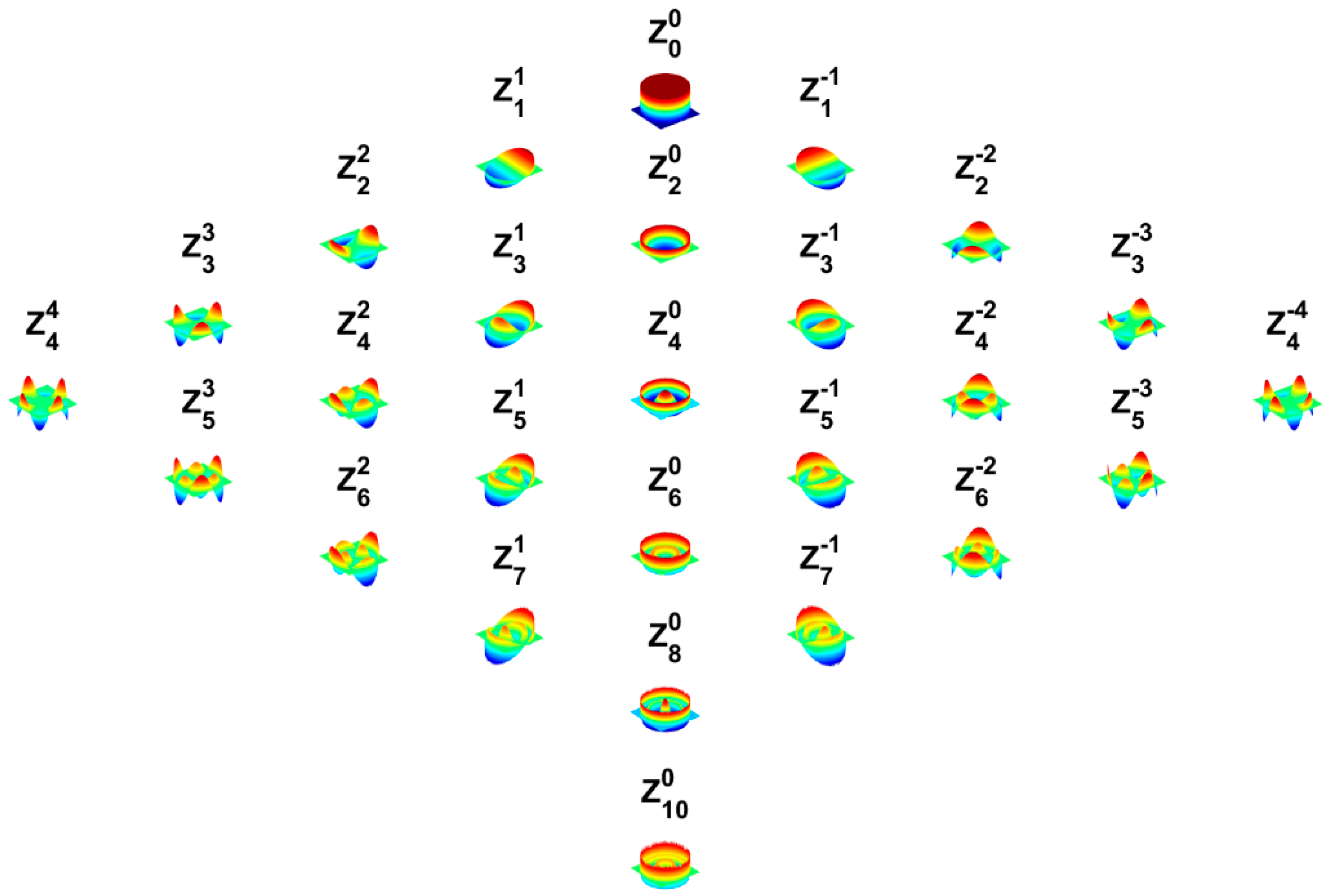
where the wavefront is described with normalized polar coordinates. A better understanding can be provided by
Table A1 in
Appendix A and by
Figure 3, which describes the indexing of Zernike polynomials and the kind of aberration associated with an index of Zernike polynomials.
4. The Space-Variant Point Spread Function
Wide-field optics is usually affected by various aberrations, such as distortion which makes the PSF of the system space-variant, i.e., the PSF changes across the field of view. It is, therefore, necessary to use a complicated model of the system’s PSF. Let us begin with a linear space-invariant optical imaging system, which can be expressed as
where
defines the shape, the size, and the transmission of the exit pupil, and
is the phase deviation of the wavefront from a reference sphere. The generalized exit pupil function is described in [
16] as
An imaging system is space-invariant if the image of a point source object changes only in position, not in the functional form [
41]. However, wide-field optical systems give images where the point source object changes both in position and in functional form. Thus, wide-field systems and their impulse responses lead to space-variant optical systems. If we consider a space-variant system, we cannot use the convolution for expressing the relation between object and image. When computing SVPSF, we have to use the diffraction integral [
6,
42]. SVPSF can then be expressed as
with a defined magnification of the system
where
z1 is the distance from the object plane to the principal plane and
z2 is the distance from the principal plane to the image plane.
5. Proposed Method
The method proposed in this paper is based on modeling the PSF of the system, and comparing it with real image data without requiring measurements of the wavefront aberrations. The fitting of the model takes place in the image plane.
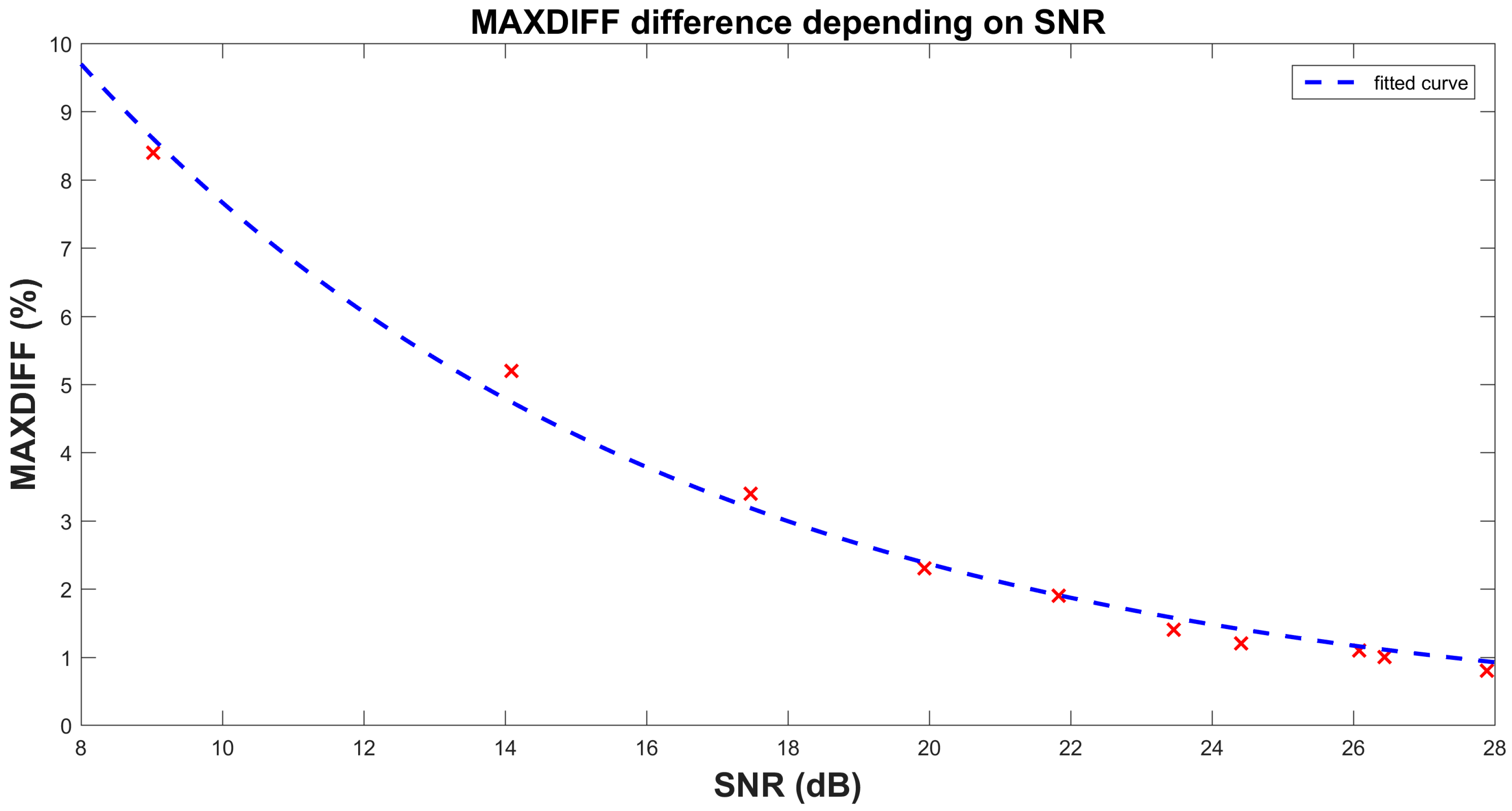
There are three conditions for acquiring the set of calibration images. The first criterion is that FWHM of the image of the light source should be sufficient for PSF estimation. The experimental results show that FWHM size greater than 5 px is enough for the algorithm. FWHM of the diffractive image of the source should be smaller than 1 px. Otherwise the diffractive function has to be added to the model of the system. The image of the 200 µm pinhole has FWHM size 0.6 µm which is less than the size of the pixel of our camera. The influence of the source shape has to be taken into account. The second criterion is the Signal-to-Noise Ratio (SNR), which should be greater than 20 dB.
Section 6 contains a comparison of results obtained with different SNR. The third criterion is that the number of test images depends on the space variance of the system, i.e., a heavily distorted optical system will require more test images to satisfy this criterion. We have to choose the distance of two different PSFs in such a way that
where
and
are the images of the point light source in the image plane.
M and
N are the sizes of the
and
images. In our example, a grid of 24 positions of the PSFs in one quadrant of the optical system is sufficient to estimate the model. The wavefront is modeled using Zernike polynomials and known optical parameters. In addition to the input image data, we need to know camera sensor parameters such as resolution, the size of the sensor and optical parameters such as the focal length (crop factor, if included), the F-number and the diameter of the exit pupil. The obtained model of the PSF of the optical system is based on the assessment of differential metrics.
We can describe the modeling of real UWFOV systems as a procedure with three main parts: the optical part, the image sensor, and the influence of the sensor noise. The space-variant impulse response
can include the influence of the image sensor (e.g., pixel shape and sensitivity profile, noise or quantization error). The sensor has square pixels with uniform sensitivity. Then, the PSF of the imaging system can be described as
where
is the PSF of the sensor and
is the PSF of the optical part. Symbol * describes the convolution.
can be calculated from the system parameters and wavefront deformations using the Fourier transform as described in Equation (13). The wavefront deformation is modeled using Zernike polynomials for the target position in the image plane (see Equation (7)). Ultra-wide field images typically have angular dependent PSF. High orders of Zernike polynomials are therefore used in the approximation. The wavefront approximation is used up to the 8th order plus the 9th spherical aberration of the expansion function. The field dependence of the coefficients is formulated in [
22]. In our work, the set of field-dependent coefficients was expanded up to the 8th order plus the 9th spherical aberration. The actual table of the used
coefficient is attached in
Appendix A as
Table A1.
Let us assume an imaging system with an unknown aberration model. We then obtain with this system a grid of
K test images of a point light sources covering the entire FOV as
Then, let
be the
d-th realization of the model in the corresponding position in the image as the original object. Sub-matrix
is the image of the point light source in the image plane, while matrix
is the sub-image model computed by our method. The size of the sub-arrays must be sufficient to cover the whole neighborhood of the point light object on the positions
.
As was mentioned above, symbols are used for image plane coordinates in the normalized optimization space, and are image plane coordinates. Note that and can be located at any point over the entire field of view. The step between the positions of the point light source has to be chosen to cover the observable difference of the acquired point. The positions of the point light source in the field of view play an important role in the convergence efficiency. In our example, we divided the field of view each 10 degrees uniformly horizontally and vertically. We therefore obtain a matrix of PSFs sufficient for a description of the model. It turned out that finer division of the FOV is not necessary and does not improve the accuracy of the model and it satisfies the condition in Equation (15).
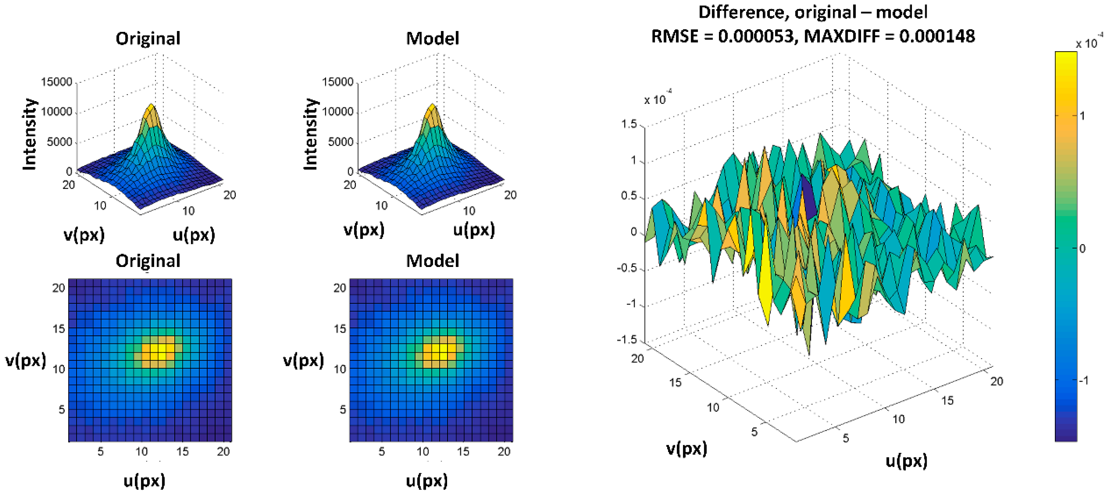
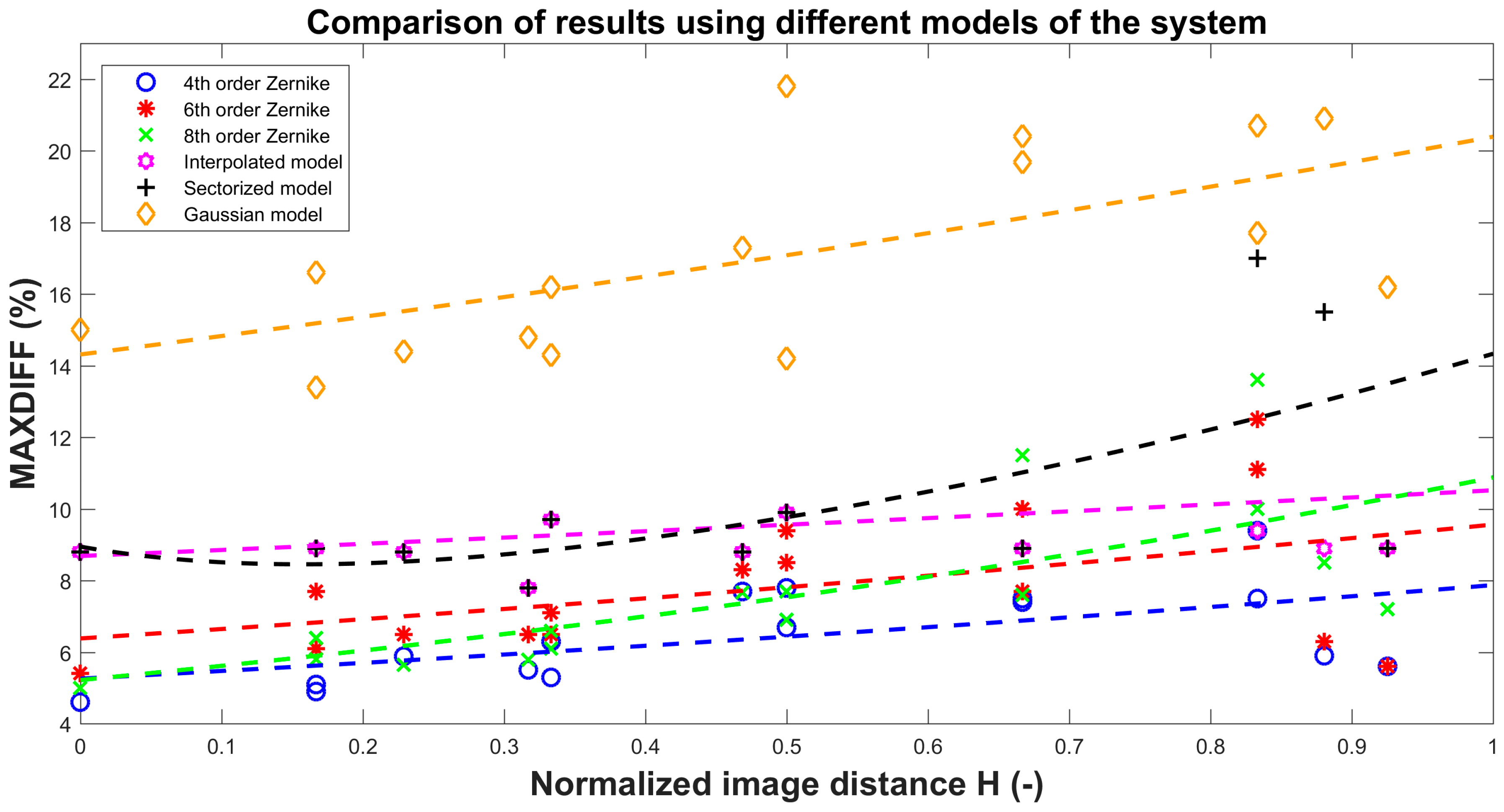
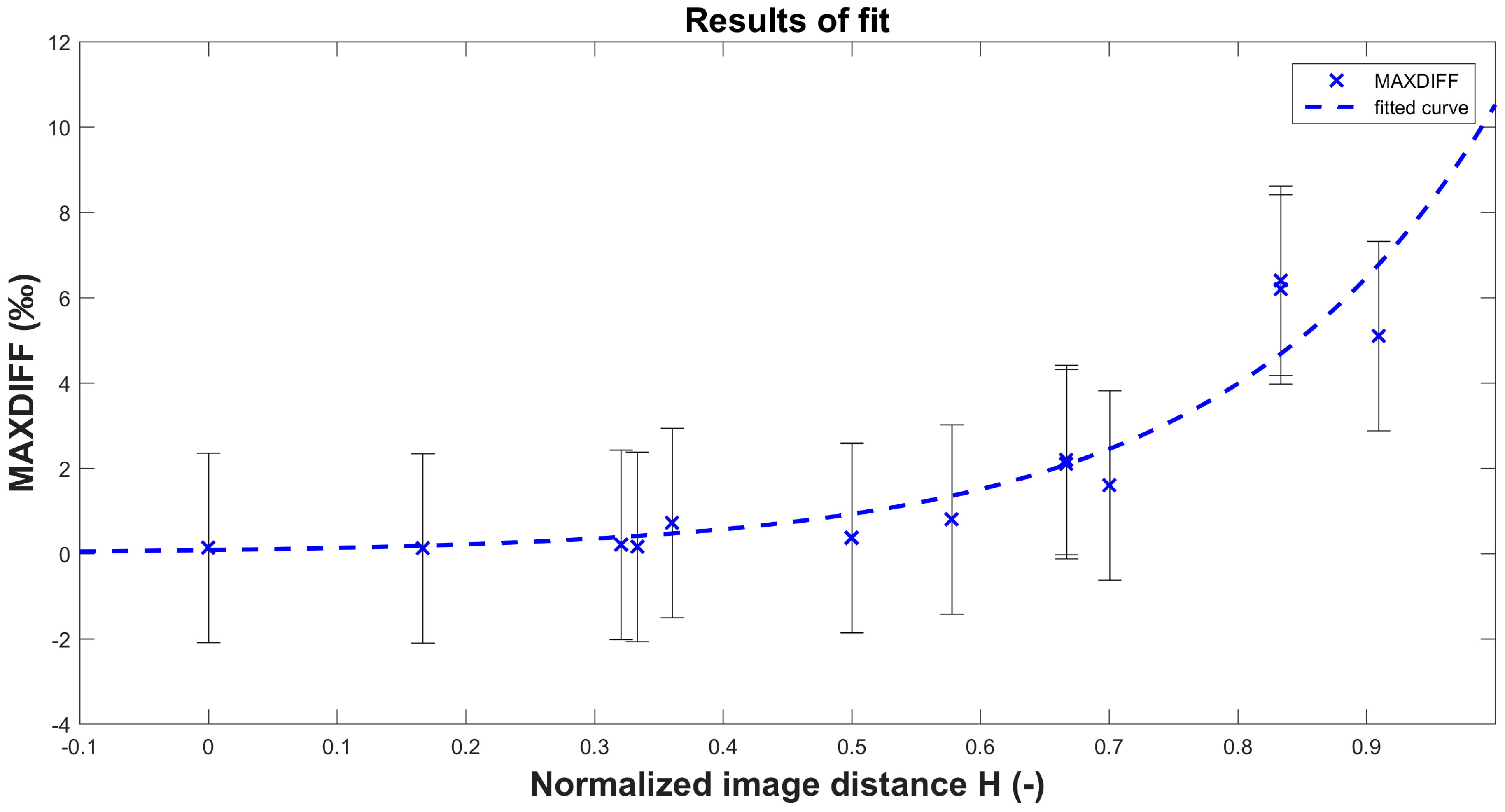
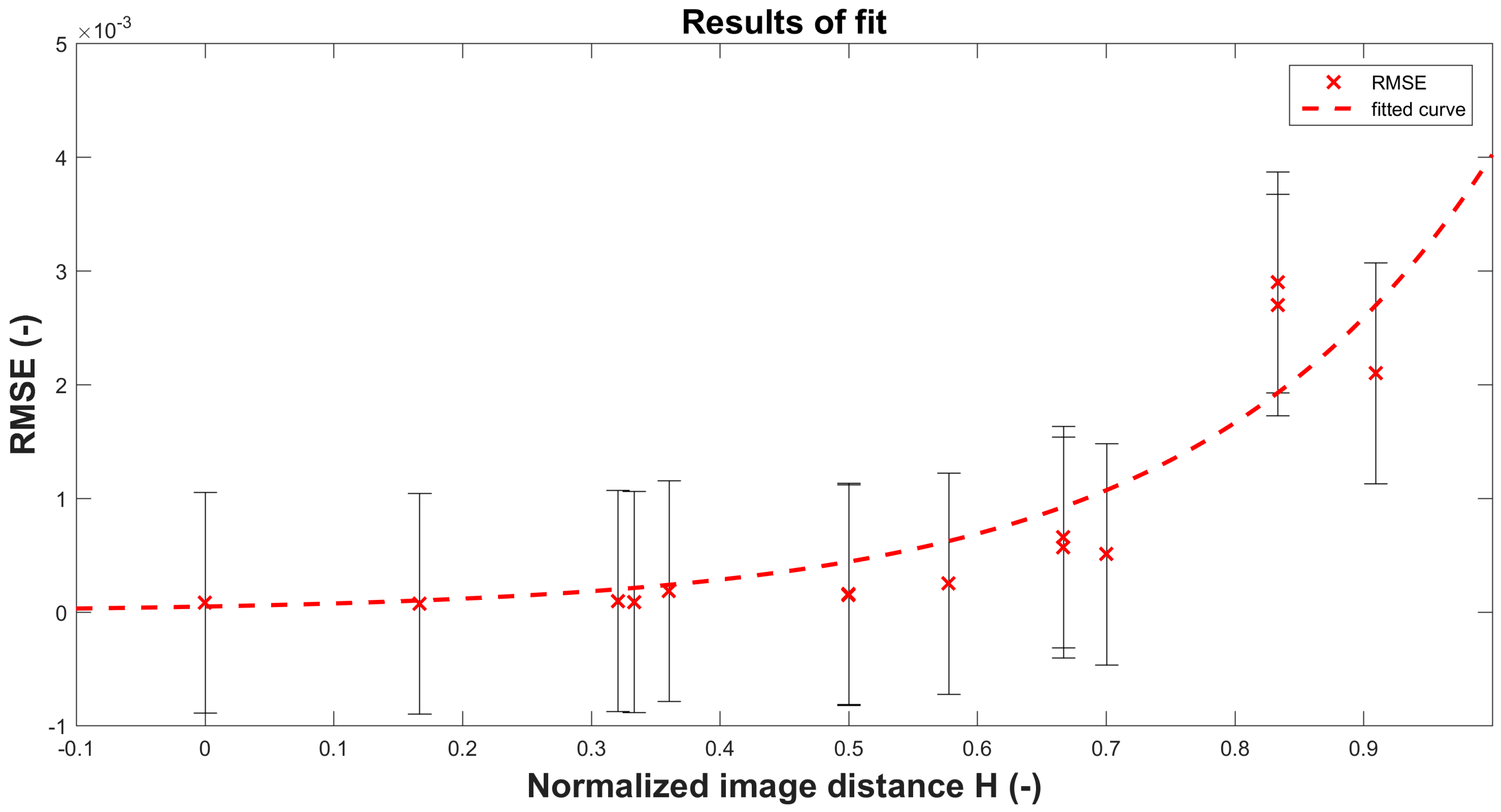
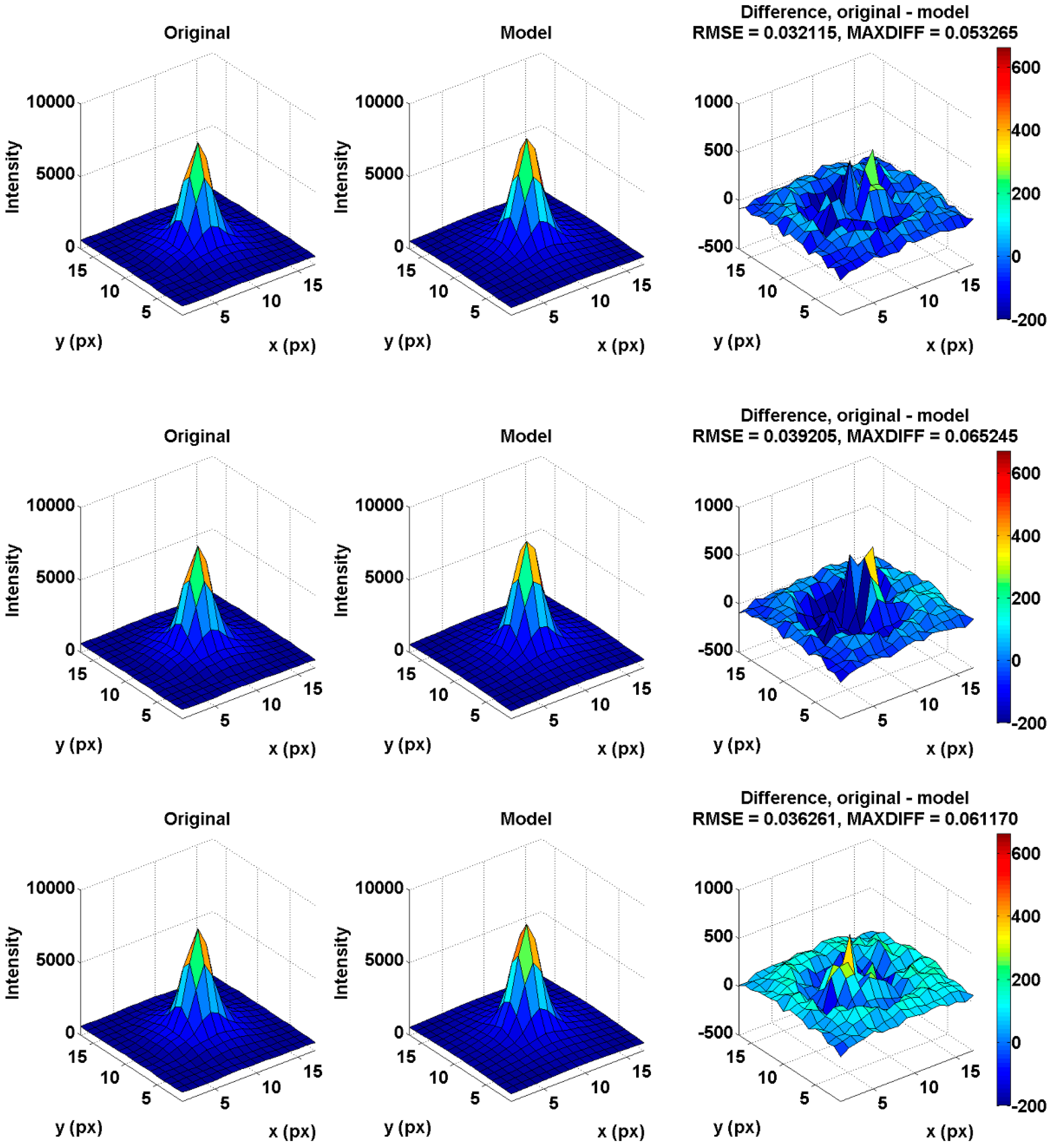
The algorithm uses two evaluation methods. The first method is based on calculating the root mean square error (RMSE) over the difference matrix in Equation (21) and optimizing the parameters and the positions for decreasing residuals. The second method is based on deducting the original and model matrix to obtain the maximum difference (MAXDIFF). Then, the residuals of this method indicate the deviation against the original matrix. The first method with RMSE calculation provides a better shape description. However, this method can result in local extremes. The reduction can be resolved by using the MAXDIFF calculation method. This method minimizes the local extremes, because it is focused on minimizing the maximum difference between the and object matrices, but the output can be a more general shape of PSF.
Let us now introduce operators
and
, which are used as descriptors of the differences between the original PSF and the model of PSF (
and
).
M and
N are the sizes of the
and
sub-arrays. The optimization parameter of the
coefficients uses the Nelder–Mead optimizing algorithm, which is described in detail in [
43]. Let
be the optimizing operator, then
where
are variables for minimizing the cost function. For multiparameter optimization tasks, the challenge is to find the global minimum of the function. Considering this issue, we can find an appropriate set of starting parameters of the fit algorithm by smart selection of on-axis points (PSFs) on which we will obtain appropriate
variables, and we will then increase the precision of our model by selecting off-axis points and improving
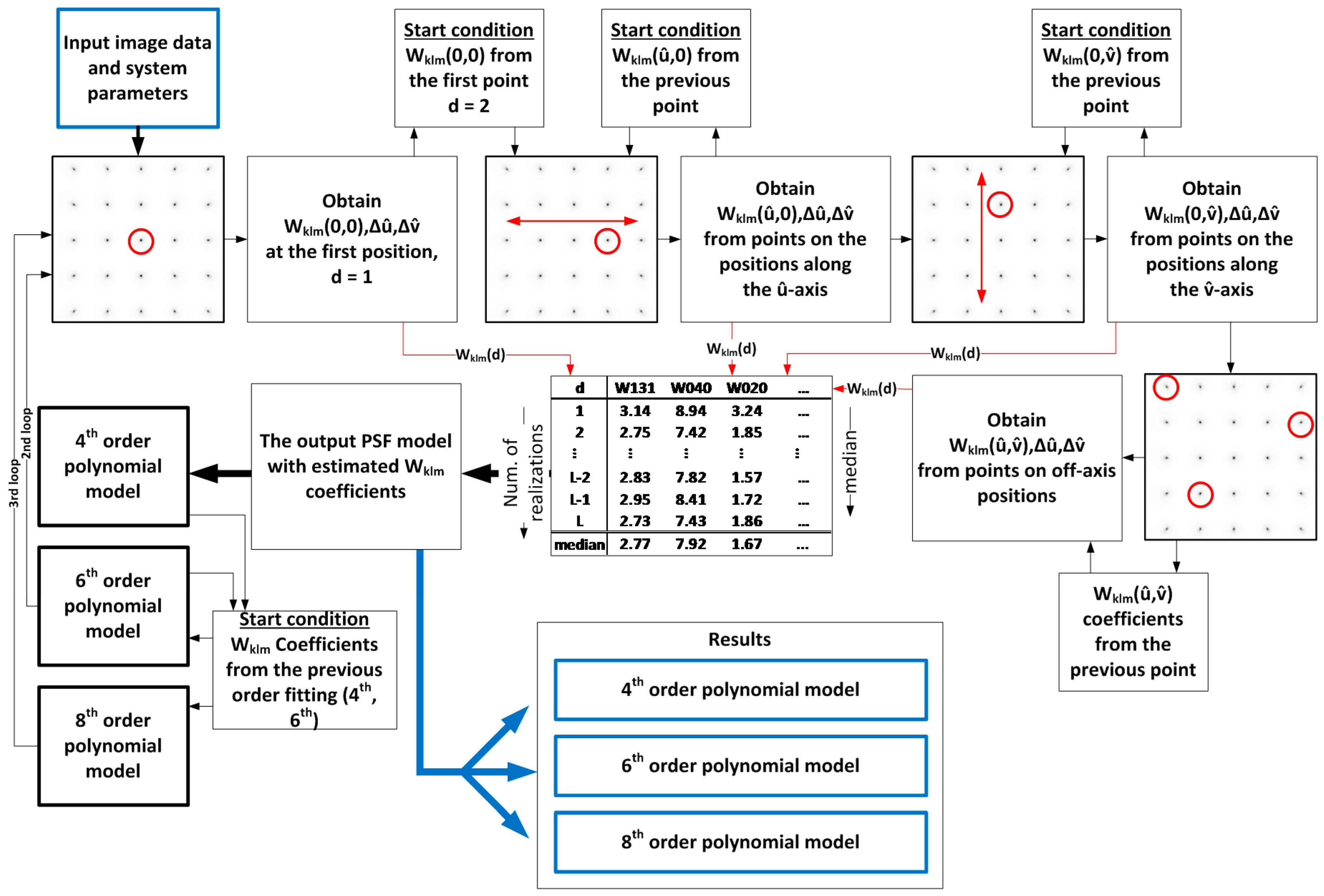
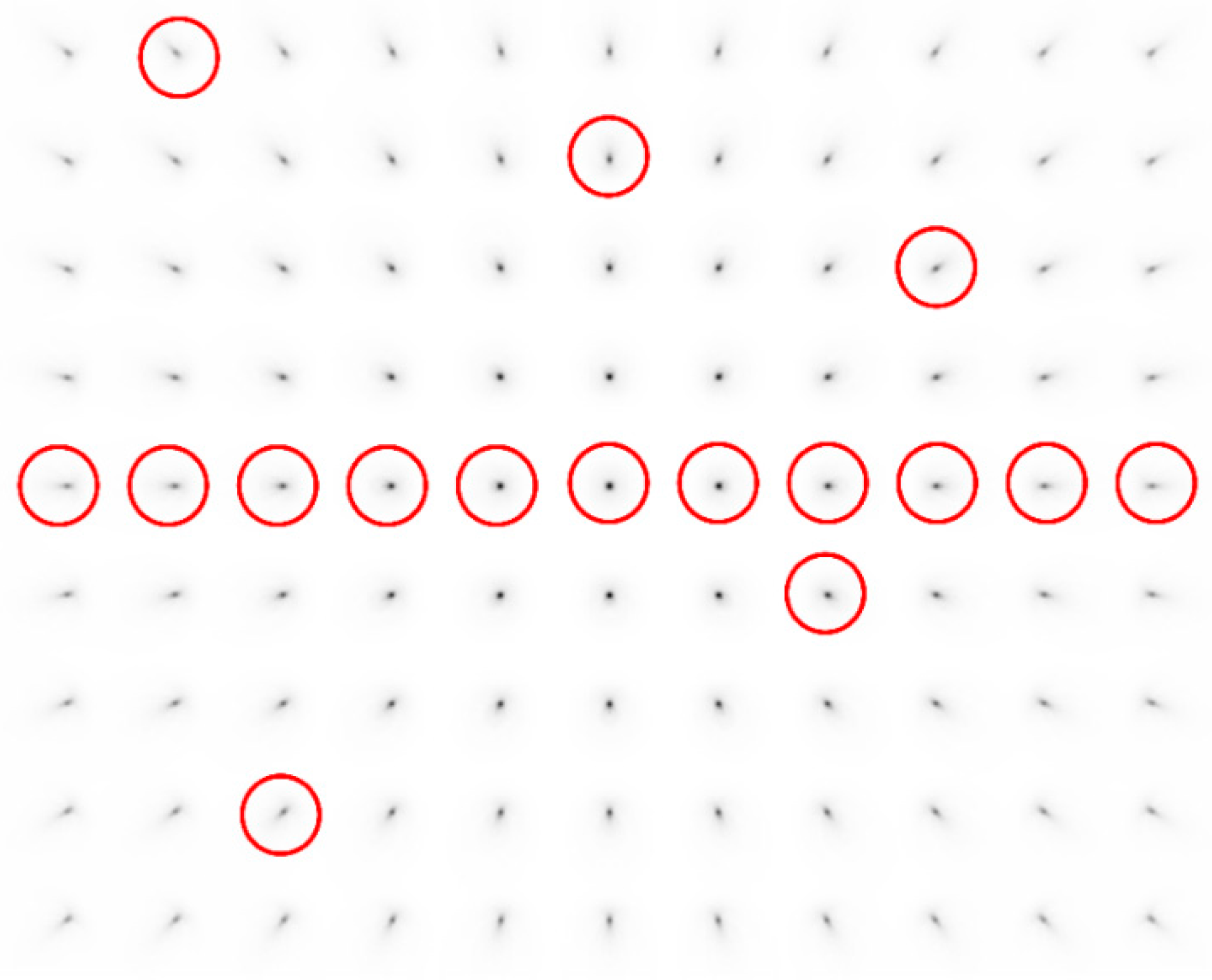
variables. The process of point selection is illustrated in
Figure 4, and the steps in the algorithm are as follows:
- ●
Select a point placed on the optical axis (this point is considered as SV aberration free).
- ○
The
optimization coefficient is based on minimizing RMSE or the MAXDIFF metrics. Then we obtain
- ○
where is the first realization of the fit, and represent the displacement of the object point in the image plane.
- ●
The next calibration point will be placed on the -axis and next to the first point.
- ○
All coefficients from the first point fit will be used as start conditions in the next step of the fit.
- ●
In the next step, we will fit all the points along the -axis by increasing distance H.
- ○
The previous result is used as the start condition for the next point.
- ●
Then, we can continue along the
-axis by increasing distance
H. This procedure gives the first view of the model.
- ○
where is the d-th realization of the fit.
- ●
After fitting all the on-axis points, we will start to fit all the off-axis points.
- ○
The example in this paper uses 24 points.
- ●
After fitting all the points, we need to evaluate the output coefficients which can describe the field dependency of our model.
- ●
We verified experimentally that the median applied to the set of estimated coefficients provides better results of the output model than other statistical methods. Thus, we need to find the median of every coefficient over all fit realizations (the number of realizations is L) of the used points. This step will eliminate extreme values of coefficients which can occur at some positions of the PSF due to convergence issues caused by sampling of the image or overfitting effects caused by high orders polynomials. Extreme values indicate that the algorithm found some local minimum of the cost function and not the global minimum. The values of the coefficients are then significantly different from the coefficients obtained in the previous position. These variations are given by the goodness of fit.
- ●
The output set of coefficients then consists of values verified over the field.
As is illustrated in
Figure 4, the described procedure repeats in every order (as defined in Equation (10)) of
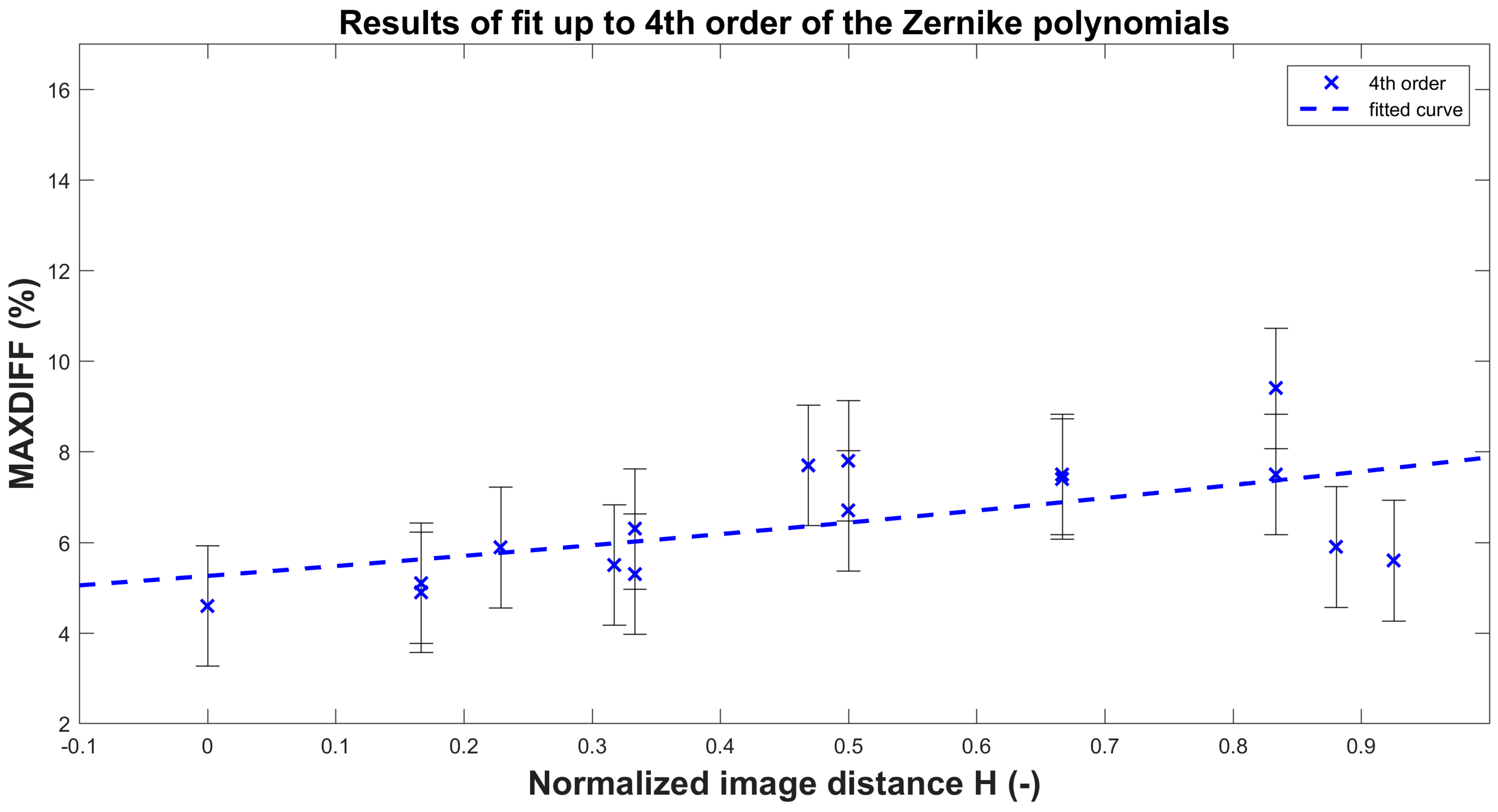
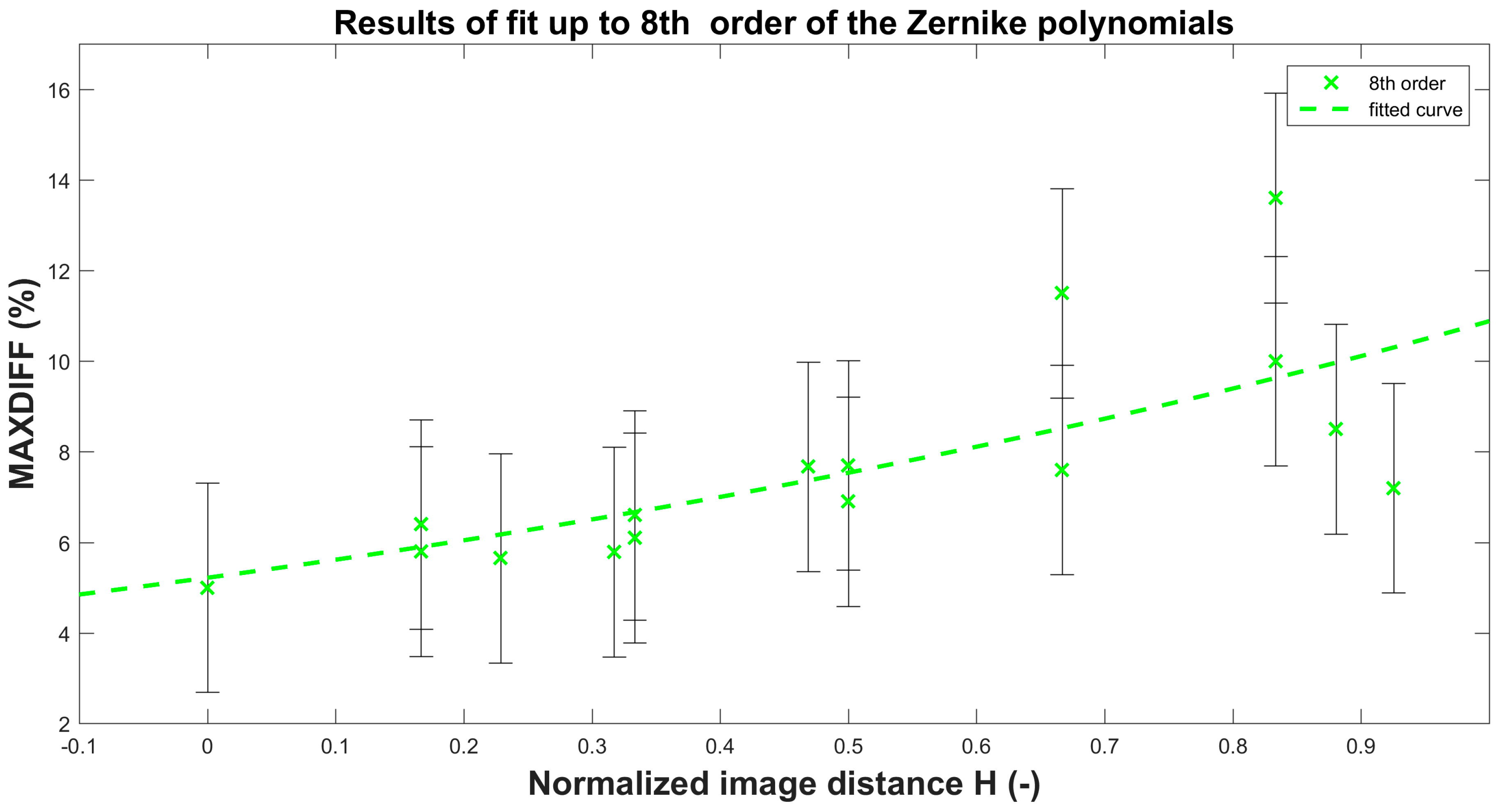
coefficients. The estimates of higher order coefficients (6th and 8th) come from lower order coefficients that have already been estimated from lower orders. If we want to describe our optical system with coefficients up to the 8th order, we will first need to obtain coefficients of the 4th order. Then, it is necessary to repeat the procedure from Equation (22) to Equation (25) of the previously described procedure assuming 4th order
coefficients as a starting condition. Following the whole procedure, we will estimate the 6th order coefficients. Then, repeating the procedure again with 6th order coefficients as a starting condition, we can finally calculate 35 coefficients of the 8th order. The result is a set of coefficients (the number of coefficients depends on the order that is used) related to the optical system with the field dependency described in
Section 3.


