A Review of Interferometric Synthetic Aperture RADAR (InSAR) Multi-Track Approaches for the Retrieval of Earth’s Surface Displacements

Featured Application

This review paper primarily aims to investigate the capabilities of the recently proposed multiple-satellite/multiple-angle Interferometric Synthetic Aperture RADAR (InSAR) combination techniques, which allow discriminating and monitoring the time evolution of three-dimensional (3-D) components of Earth’s surface deformations. Such methods are nowadays being widely applied, mostly in areas characterized by the presence of significant deformation signals (for instance, due to massive volcanic or seismic episodes) and to less extent in regions with low-to-moderate deformation signals. This work intends to provide insights on theoretical aspects of multi-pass InSAR techniques and their applicability for the monitoring of a heterogeneous class of deformation phenomena.

Abstract

Synthetic Aperture RADAR Interferometry (InSAR) provides a unique tool for the quantitative measurement of the Earth’s surface deformations induced by a variety of natural (such as volcanic eruptions, landslides and earthquakes) and anthropogenic (e.g., ground-water extraction in highly-urbanized areas, deterioration of buildings and public facilities) processes. In this framework, use of InSAR technology makes it possible the long-term monitoring of surface deformations and the analysis of relevant geodynamic phenomena. This review paper provides readers with a general overview of the InSAR principles and the recent development of the advanced multi-track InSAR combination methodologies, which allow to discriminate the 3-D components of deformation processes and to follow their temporal evolution. The increasing availability of SAR data collected by complementary illumination angles and from different RADAR instruments, which operate in various bands of the microwave spectrum (X-, L- and C-band), makes the use of multi-track/multi-satellite InSAR techniques very promising for the characterization of deformation patterns. A few case studies will be presented, with a particular focus on the recently proposed multi-track InSAR method known as the Minimum Acceleration (MinA) combination approach. The presented results evidence the validity and the relevance of the investigated InSAR approaches for geospatial analyses.

1. Introduction

Synthetic Aperture RADAR (SAR) is a coherent active microwave remote sensing instrument [1,2,3], whose capability to efficiently map the scattering properties of the Earth’s surface is well documented [4,5,6]. A SAR sensor—which can be mounted on board an aircraft or satellite—has a side-looking illumination direction and can accurately retrieve the location of an object (target) relative to the position of the platform where the sensor is mounted. Both the acquisition geometry and the physical characteristics of the imaged scene contribute to the formation of the received backscattered RADAR signal (echo) which, correctly processed, leads to the reconstruction of a complex-valued high-resolution microwave image of the observed area [2]. SAR is an active imaging sensor, i.e., it does not need an external energy source to work. Moreover, since it typically operates in the microwave region of the electromagnetic spectrum, it can be used efficiently in any meteorological condition (i.e., in the presence of a significant clouds’ cover) and with a full day-and-night operational capability. As a consequence of its flexibility, SAR technology mostly improved over the last decades, thus developing further technologies based on the use of SAR data for the detection and monitoring of several geophysical phenomena [7,8,9,10,11,12,13,14,15,16]. Among these techniques, the SAR interferometry [13,14,15,16] plays a major role in the study of the dynamic of Earth’s crust, thus permitting the monitoring of the surface movements. Deformations can be induced by several geophysical phenomena, such as the extensive fractures due to big earthquakes [17,18,19], pre-seismic deformations [20], slow-moving landslides [21,22,23,24], the eruptions of active volcanoes [25,26,27,28]. Human beings also severely contribute to the changes in the environment. In this framework, InSAR can monitor the modifications over time of highly urbanized zones by measuring the settlements of buildings, private and public facilities [29,30,31]. The results of these investigations are useful for city planners and local authorities to mitigate the urban risk and design effective plans of cities development.

This review paper will first address the fundamentals of InSAR technology and, then, will provide an overview of recently proposed multi-track/multi-satellite InSAR-based methodologies [32], which allow the detection and the continuous monitoring of the three-dimensional shape of deformation phenomena.

The paper is organized as follows. Section 2 illustrates the InSAR rationale, emphasizing key strengths and potential limitations. Section 3 provides an overview of the multi-pass InSAR techniques and Section 4 describes, with more details, the recently proposed minimum acceleration InSAR combination method [32]. The results of a few experiments will also be presented. Future perspectives on the use of InSAR and multi-satellite InSAR methodologies will be finally provided in Section 5.

2. Overview of InSAR Methodology

One of the principal applications of the SAR technology is represented by the SAR interferometry (InSAR) technique [13,14,15,16]. It relies on the measurement of the phase difference between two (or more) complex-valued SAR images, acquired from different orbital positions and/or at different times. In principle, different distributions of the receiving/transmitting antennas define distinctive interferometric configurations. In particular, conventional mono-static InSAR configurations involve the use of two antennas observing the investigated scene:

➢

at the same time and from different positions, spaced in the across-track direction (across-track interferometry);

➢

at different times and from the same position (along-track interferometry) [33,34];

➢

at different times and from different orbital positions (repeat-pass across-track interferometry).

Bi-static and multi-static InSAR interferometry configurations, where receiving and transmitting antennas are on board different moving platforms, have also been explored [35,36,37]. Such field of research, within InSAR framework, represents one of the most promising lines of development of InSAR technology.

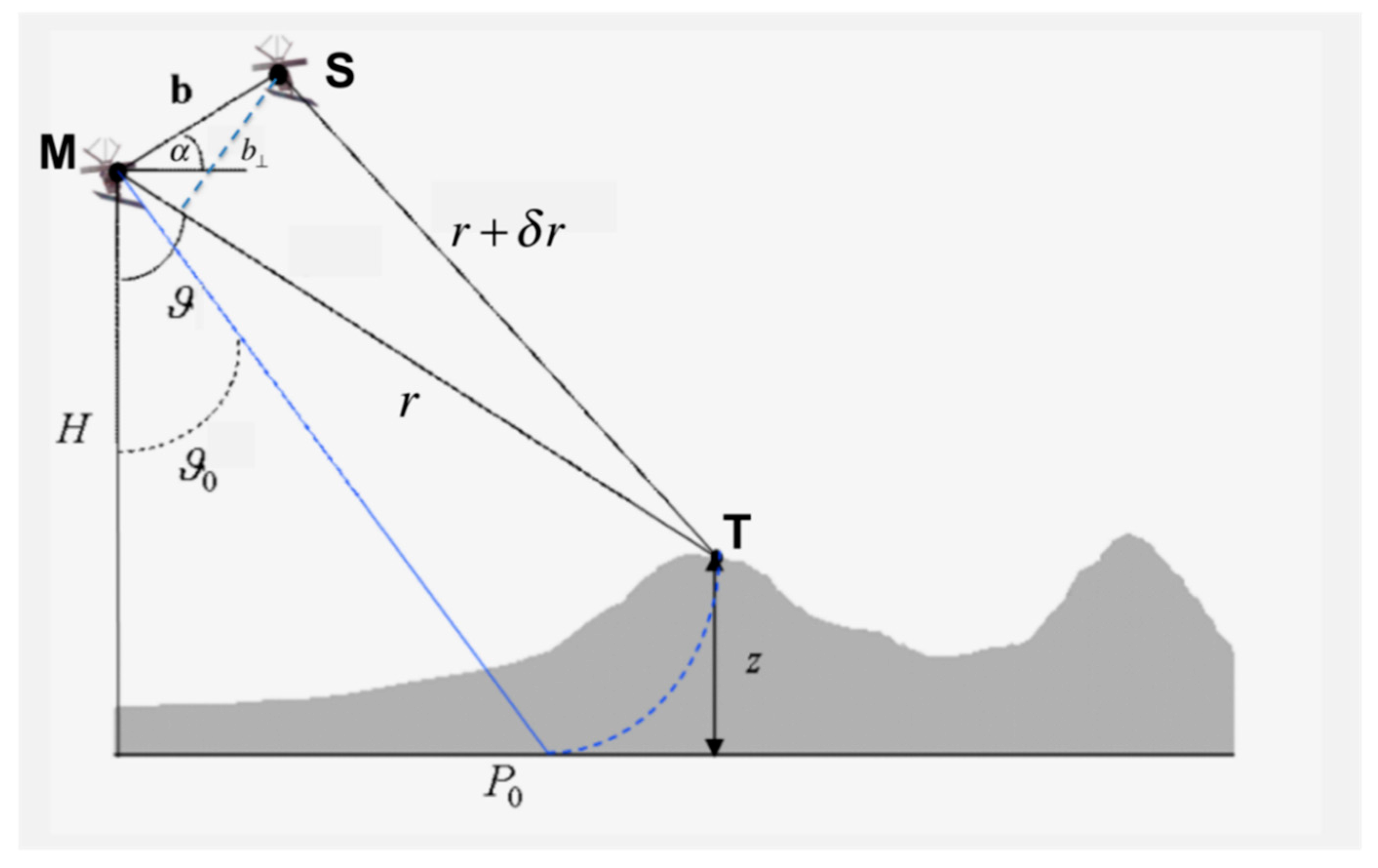
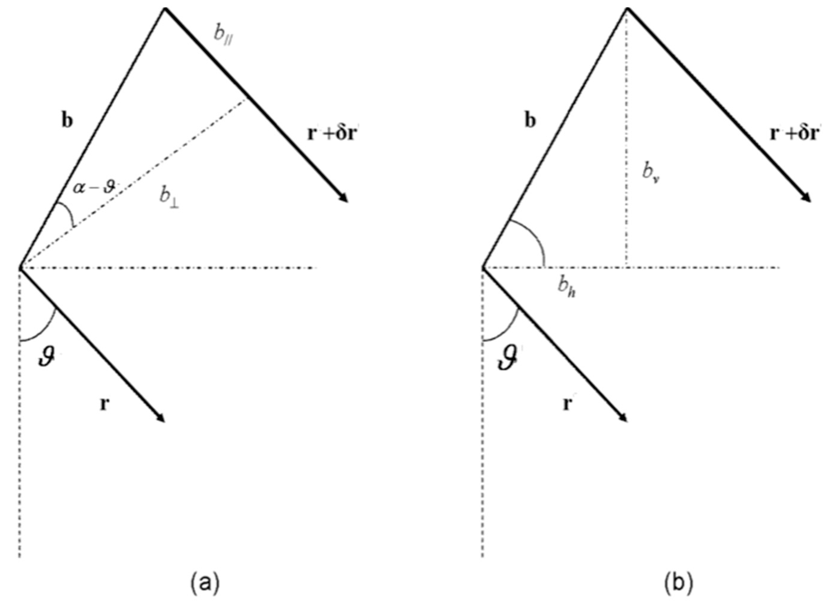
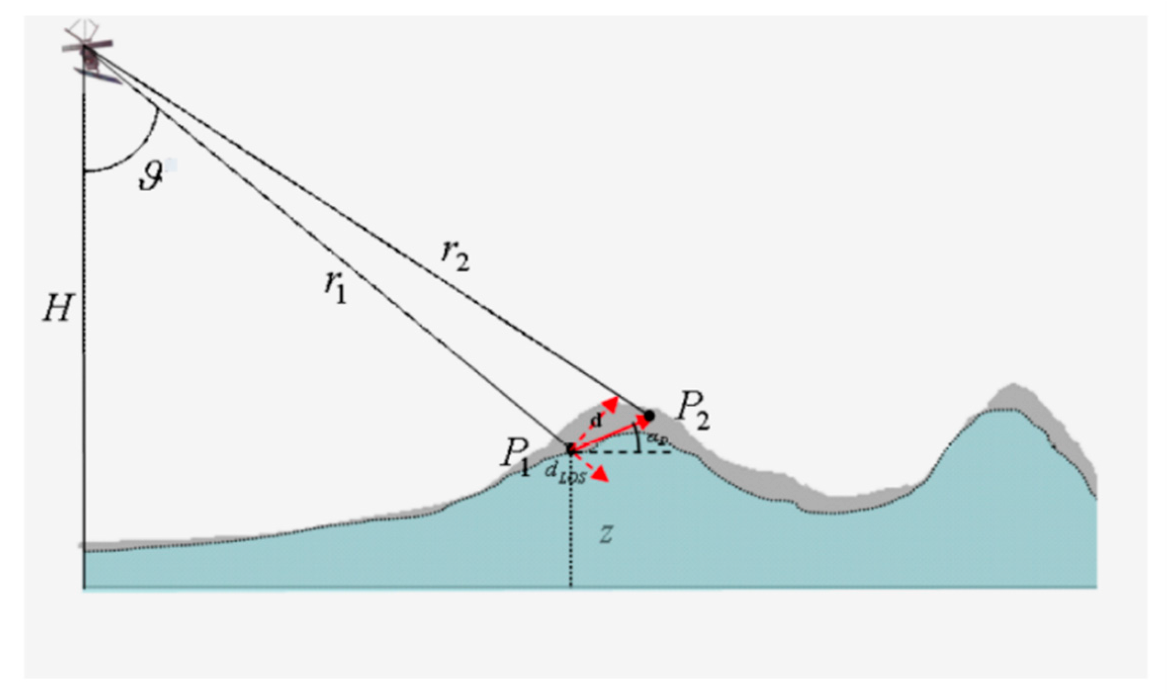
2.1. InSAR Technique for the Estimation of Height Topography

In this review, we concentrate on the repeat-pass across interferometry. As earlier anticipated, such technology allows the measurement of geomorphological characteristics of the ground, such as the topography height and the modifications of the Earth’s surface, due to earthquakes, volcano eruptions or other geophysical phenomena. Historically, InSAR has been mostly used for the measurement of the ground topography [38,39,40]. To understand how InSAR works, let us refer to the imaging geometry depicted in Figure 1 and suppose the involved RADAR system acquires two SAR images over the same area. The first SAR image (i.e., commonly referred to as master image) is taken from the orbital position labelled to as M. The second image (i.e., the so-called slave image) is captured from the orbital position marked as S, located at a distance b (referred to as baseline) from M. Notice that in the plane orthogonal to azimuth direction the two SAR antennas are separated by the baseline vector b, which can be decomposed into either its parallel/perpendicular $\left(b_{//},b_{\perp }\right)$ or horizontal/vertical $\left(b_h,b_v\right)$ components, respectively. Taking into account geometric considerations and by direct inspection of Figure 1 and Figure 2, it is easy to demonstrate the validity of the following mathematical relationships:

$$\{\begin{array}{c}{b}_{\perp }=b\cos \left(\mathsf{\vartheta }-\mathsf{\alpha }\right)=b_h\cos \mathsf{\vartheta }+b_v\sin \mathsf{\vartheta }\\ b_{//}=-b\sin \left(\mathsf{\vartheta }-\mathsf{\alpha }\right)=b_h\sin \mathsf{\vartheta }-b_v\cos \mathsf{\vartheta }\\ b_h=b\cos \mathsf{\alpha }=b_{\perp }\cos \mathsf{\vartheta }+b_{//}\sin \mathsf{\vartheta }\\ b_v=b\sin \mathsf{\alpha }=b_{\perp }\sin \mathsf{\vartheta }-b_{//}\cos \mathsf{\vartheta }\end{array}$$

(1)

where ϑ and α are the satellite side-looking angle and the inclination angle of the baseline vector with respect to the horizontal plane, respectively. Equations (1) are fundamental to calculate the sensitivity of InSAR measurements to deformation measurements, as subsequently outlined in this Section. If we assume that the RADAR system has an infinite bandwidth, the master and slave complex-valued SAR images can be mathematically represented, pixel-by-pixel, as follows:

$${\widehat{\mathsf{\gamma }}}_1={\mathsf{\gamma }}_1\exp \left[-j\frac{4\mathsf{\pi }}{\mathsf{\lambda }}r\right]$$

(2)

$${\widehat{\mathsf{\gamma }}}_2={\mathsf{\gamma }}_2\exp \left[-j\frac{4\mathsf{\pi }}{\mathsf{\lambda }}\left(r+\mathsf{\delta }r\right)\right]$$

(3)

where ${\mathsf{\gamma }}_1$ and ${\mathsf{\gamma }}_2$ are the complex reflectivity functions of the master and slave data, respectively and λ denotes the effective RADAR wavelength. The interferometric phase map (called an interferogram) is formed, on a pixel-by-pixel basis, starting from the two co-registered (complex-valued) master and slave SAR images. Notice that the misalignment of the second image is precisely due to the path difference between the two RADAR signals.

Precisely for this reason, it is needed to properly co-register the images to represent the two SAR images in the same reference geometry [41,42]. In Equations (2) and (3), for the sake of simplicity, we have not considered the presence of any possible noise signals that corrupt the SAR signals. A comprehensive overview of the sources of noise associated with SAR images falls beyond the scopes of this review paper. Nonetheless, the Section 2.2 addresses the problem of noise corrupting interferometric SAR signal. Let us first discuss the rationale of the interferometry SAR technique. Taking into account Equations (2) and (3), we obtain, for each RADAR pixel, the phase difference between the two SAR images by merely multiplying the first image (master) by the complex conjugate of the second image (slave) and, then, by extracting its phase term:

$$C={\widehat{\mathsf{\gamma }}}_1{\widehat{\mathsf{\gamma }}}_2^{*}=\left|{\widehat{\mathsf{\gamma }}}_1{\widehat{\mathsf{\gamma }}}_2\right|\exp \left[j\left(\frac{4\mathsf{\pi }}{\mathsf{\lambda }}\mathsf{\delta }r+\measuredangle {\mathsf{\gamma }}_1-\measuredangle {\mathsf{\gamma }}_2\right)\right]$$

(4)

where the symbol (*) denotes the complex conjugate operation and the symbol $\measuredangle$ represents the phase extraction operation. From Equation (4), assuming that the electromagnetic-wave scattering mechanism on the ground has not changed between the two passages of the sensor over the illuminated area (this requirement could be directly accomplished if a single-pass configuration was considered), we get:

$$C={\widehat{\mathsf{\gamma }}}_1{\widehat{\mathsf{\gamma }}}_2^{*}={\left|\widehat{\mathsf{\gamma }}\right|}^2\exp \left[j\frac{4\mathsf{\pi }}{\mathsf{\lambda }}\mathsf{\delta }r\right]$$

(5)

and its full phase term (i.e., not restricted to the [−π, π] interval) represents the so-called interferometric phase:

$$\mathsf{\phi }=\frac{4\mathsf{\pi }}{\mathsf{\lambda }}\mathsf{\delta }r$$

(6)

Taking into account the acquisition geometry illustrated in Figure 1 and Figure 2 and in the application of the cosine’s rule to the MST triangle depicted in Figure 1 [41], it is straightforward to demonstrate that:

$$r+\mathsf{\delta }r=\sqrt{b^2+r^2-2br\sin \left(\mathsf{\vartheta }-\mathsf{\alpha }\right)}\simeq r\prime -b\sin \left(\mathsf{\vartheta }-\mathsf{\alpha }\right)$$

(7)

Accordingly, the interferometric phase, see (6), can be written as:

$$\mathsf{\phi }\simeq -\frac{4\mathsf{\pi }}{\mathsf{\lambda }}b\sin \left(\mathsf{\vartheta }-\mathsf{\alpha }\right)=\frac{4\mathsf{\pi }}{\mathsf{\lambda }}{b}_{//}$$

(8)

where $b_{//}$ is the parallel baseline component, see Equation (1).

At this stage, the problem to be addressed is the recognition of the interferometric phase dependency upon the surface topography and the subsequent estimation of the error budget of the InSAR-based topographic measurements. To this aim, let us refer again to the geometry of the problem sketched in Figure 1 and we expand Equation (8) around the angular position ϑ = ϑ₀, which represents the side-looking angle that corresponds to the case when Earth’s surface is flat (i.e., z = 0). Therefore:

$$\mathsf{\phi }\simeq -\frac{4\mathsf{\pi }}{\mathsf{\lambda }}b\left[\sin \left({\mathsf{\vartheta }}_0-\mathsf{\alpha }\right)+\cos \left({\mathsf{\vartheta }}_0-\mathsf{\alpha }\right)\left(\mathsf{\vartheta }-{\mathsf{\vartheta }}_0\right)\right]$$

(9)

The target height, namely z, is related to the side-looking angle ϑ and to the satellite height H as $z=H-r\cos \mathsf{\vartheta }$.

Hence:

$$\frac{\partial z}{\partial \mathsf{\vartheta }}=r\sin \mathsf{\vartheta }\to \frac{\partial \mathsf{\vartheta }}{\partial z}=\frac{1}{r\sin \mathsf{\vartheta }}\to \mathsf{\vartheta }-{\mathsf{\vartheta }}_0=\frac{z}{r\sin \mathsf{\vartheta }}$$

(10)

Finally, the interferometric phase can be seen as composed of two distinctive terms, as follows:

$$\mathsf{\phi }\simeq -\frac{4\mathsf{\pi }}{\mathsf{\lambda }}b\sin \left({\mathsf{\vartheta }}_0-\mathsf{\alpha }\right)-\frac{4\mathsf{\pi }}{\mathsf{\lambda }}\frac{b_{\perp }}{r\sin \mathsf{\vartheta }}z$$

(11)

where the mathematical relation $b_{\perp }=b\cos \left(\mathsf{\vartheta }-\mathsf{\alpha }\right)$ (see (1)) has been used.

The first term on the right-end side of Equation (11) represents the so-called flat-Earth phase contribution, i.e., the phase that is obtained when the topographic profile is entirely flat (z = 0). The second term relates the interferometric phase to the surface height z. By Equation (11), it is simple to understand that the interferometric phase is proportional to the height through the value of the perpendicular baseline of the interferometric data pair. Accordingly, the larger the perpendicular baseline, the more accurate the estimate of the topography, as clarified by the following Equation (12) that relates the standard deviation of the phase measurement (i.e., the error of the InSAR phase measurement)—namely σ_ϕ—to the standard deviation of the InSAR-driven height measurements, namely σ_z:

$${\mathsf{\sigma }}_z=-\frac{\mathsf{\lambda }}{4\mathsf{\pi }}\frac{r\sin \mathsf{\vartheta }}{b_{\perp }}{\mathsf{\sigma }}_{\mathsf{\phi }}$$

(12)

By using the parameters of the C-band ASAR RADAR instrument mounted on board the ENVISAT satellite of the European Space Agency (ESA), we have evaluated the accuracy of the height measurement in a real context. Note that the ENVISAT/ASAR instrument operated from 2002 to 2010 with a wavelength of 5.6 cm, the scenes were imaged with an average side-looking angle of about 23° and the sensor-to-target distance, namely r, was approximately 800 km. Figure 3 and Figure 4 depict the plot of the standard deviation of the height measurement (as calculated by Equation (12)) vs. the perpendicular baseline and the standard deviation of the interferometric phase, respectively. The accuracy of InSAR phase, however, depends on the perpendicular baseline of the interferogram. Unfortunately, an increase in the perpendicular baseline, which would be beneficial for reducing the standard deviation of the height measurement by Equation (12), is responsible for increasingly severe decorrelation noise artefacts [41,43,44,45] (see Section 2.2 for details) in the generated map of the interferometric phase. Accordingly, the use of very large baseline interferograms limits the efficacy of InSAR-based height measurement. For this reason, in practice, a compromise arises for establishing a criterion for the selection of the optimal baseline separation between orbits for InSAR applications. Height accuracy can also be calculated with respect to the components of the baseline vector. To do that, we observe that, by using Equations (7) and (11) (neglecting the flat-Earth term contribution), the topography can be expressed as a function of the parallel baseline component as:

$$z=\frac{r\sin \mathsf{\vartheta }}{b_{\perp }}{b}_{//}$$

(13)

and, making use of Equations (1), we get:

$$z=\frac{r{\sin }^2\mathsf{\vartheta }}{b_{\perp }}{b}_h-\frac{r\sin \left(2\mathsf{\vartheta }\right)}{2b_{\perp }}{b}_v$$

(14)

Therefore, the standard deviation of the topography can also be expressed as follows:

$$\begin{array}{l}{\mathsf{\sigma }}_z=\frac{r{\sin }^2\mathsf{\vartheta }}{b_{\perp }}{\mathsf{\sigma }}_{b_h}\\ {\mathsf{\sigma }}_z=\frac{r\sin \left(2\mathsf{\vartheta }\right)}{2b_{\perp }}{\mathsf{\sigma }}_{b_v}\end{array}$$

(15)

Finally, another frequently-used measure of the interferometric performance for the estimation of height topography is the so-called height ambiguity, which represents the amount of height change leading to a 2π-change of the interferometric phase, which can be easily derived from Equation (12) by imposing σ_ϕ = 2π, as:

$$z_{2\mathsf{\pi }}=\left|-\frac{\mathsf{\lambda }r\sin \mathsf{\vartheta }}{2b_{\perp }}\right|$$

(16)

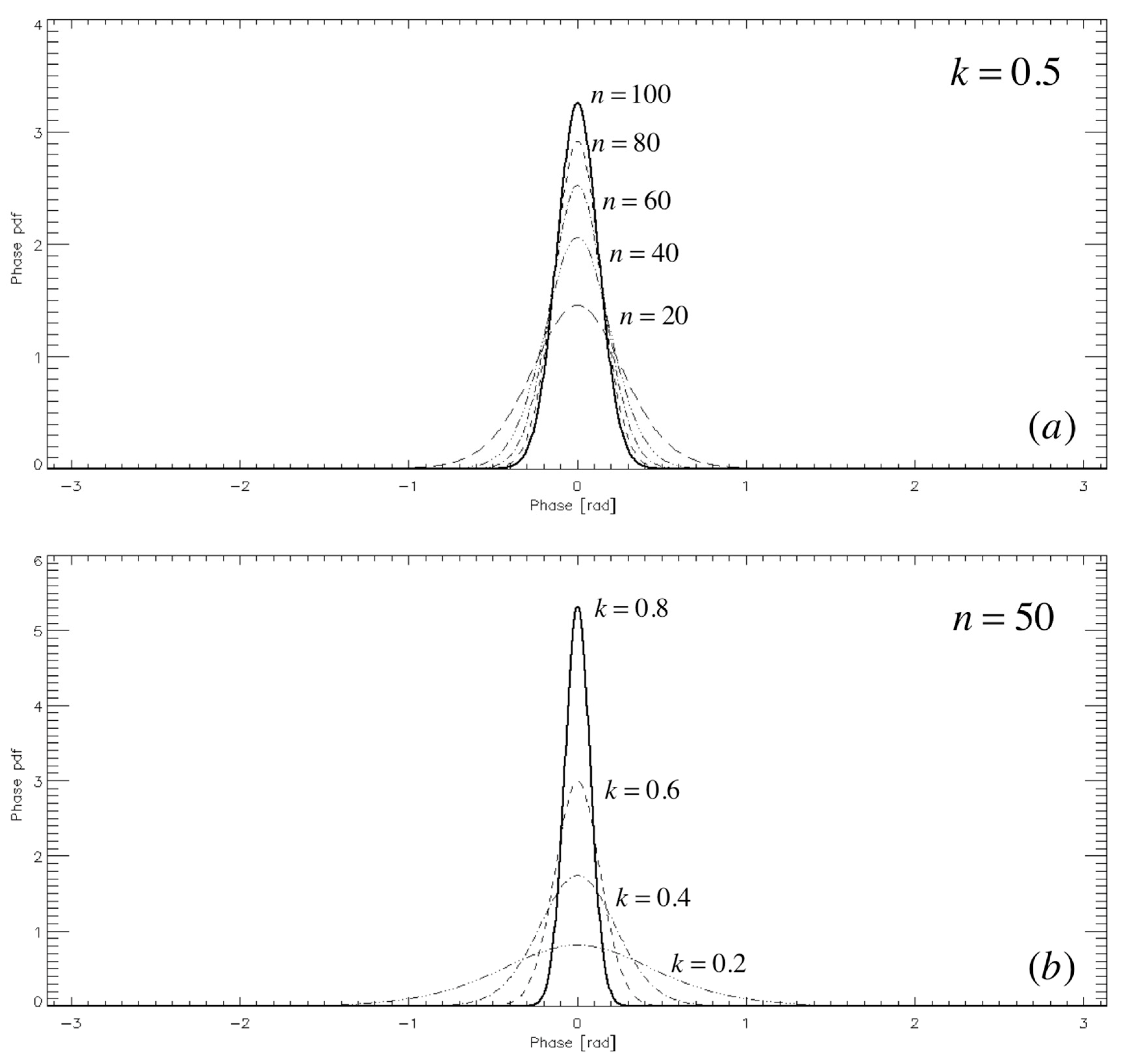
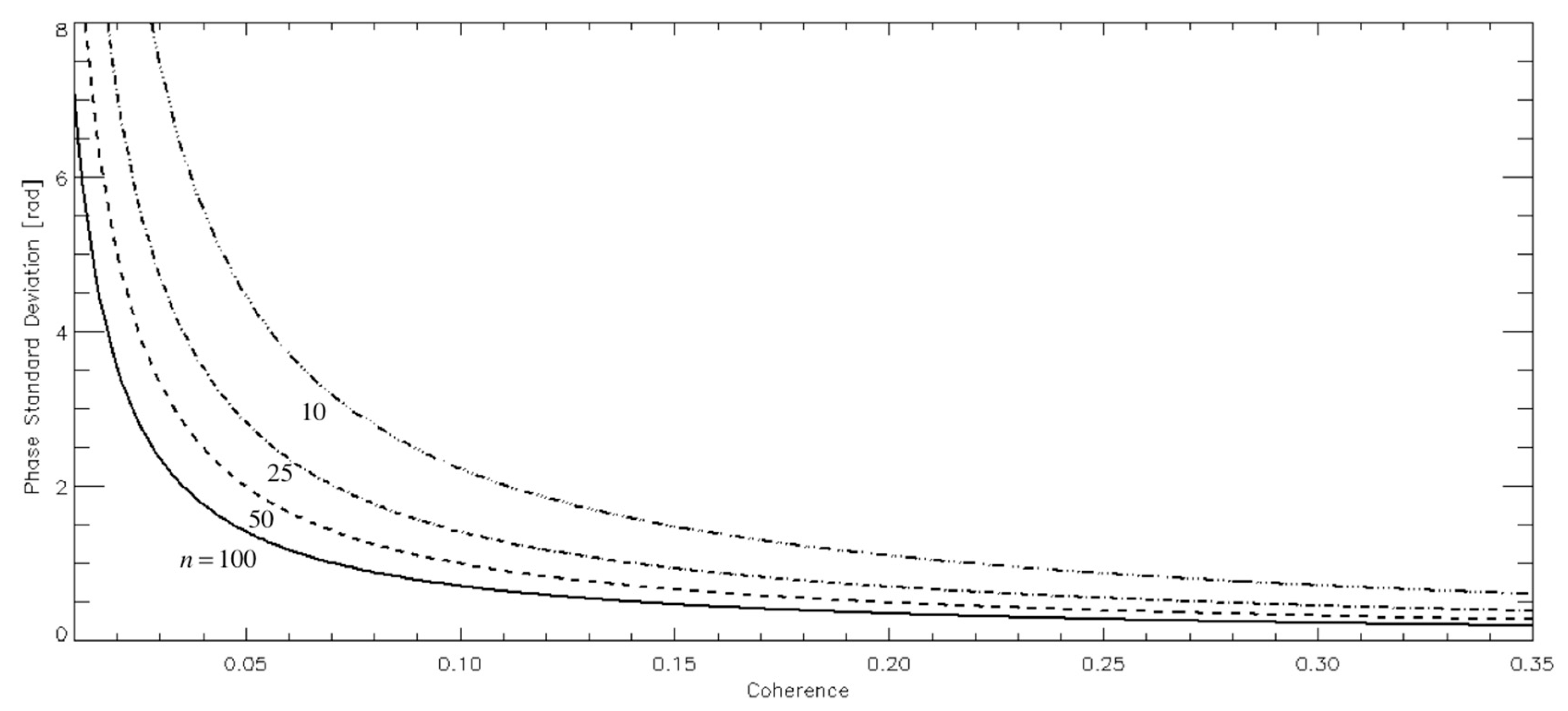
2.2. Noise Signals Corrupting SAR Interferograms

This subsection shortly addresses the issue of characterizing the noise that corrupts the interferometric SAR signal. The focus is mostly on the noise signals that characterize the interferometric phase. Accordingly, we neglect the effect of additional noise signals corrupting the complex-valued SAR signals that are ascribable to inaccurate pre-processing of SAR data. To this class belong the errors due to an incorrect focusing of SAR raw data [41,46,47,48], the presence of uncompensated radio frequency interference (RFI) signatures in the focused SAR imagery [49,50,51], or other possible causes of disturbances in the complex SAR signal. These effects globally increase the level of noise in the generated interferograms but their full characterization is outside the aim of this review paper. Here, we only spend a few words about the effect of uncompensated RFI signals in the two interfering master and slave SAR acquisitions. RFI artefacts are due to electromagnetic interference signals emitted by civil and military communication systems at the operational radar frequency in many areas of the world [49,50]. These artefacts are known to be more prominent at low frequency (L-band). For instance, SAR raw data collected by the Japanese L-band PALSAR systems are affected by such mistakes, which are mostly compensated during pre-processing and focusing of SAR data at ground stations before the delivering to users. At higher frequencies, RFI events have occurred but they are somewhat limited. ESA has reported some limited RFI events at C-band (although there is evidence they are increasing), whereas at X-band they have not been reported so frequently to represent a real problem [50]. Uncompensated RFI artefacts appear as various kinds of bright linear features in the azimuth-time range frequency domain [51]. Incoherent RFI is filtered out (at most) by the matched-filter used for focusing the SAR images. However, high-power RFI signals might be filtered during focusing step and they require proper RFI filters to be implemented [52,53,54]. Uncompensated RFI can increase the noise level in the phase signature of SAR images at L-band [55]. As said, however, the characterization of the RFI effects falls outside the limits of our investigation. Interested readers can find details on the RFI sources and the developed algorithms for their mitigation in SAR images, in [51] and the references listed therein.

This subsection aims to get an estimate of the error-budget associated to the InSAR measurement of the terrain height topography. As said, the standard deviation of the height is linked to the standard deviation of the InSAR phase σ_ϕ by Equation (12). Our analysis moves from the basic observation that, in the interferometric processing, the conjugate multiplication of the two co-registered master and slave SAR images yields the complex interferogram:

$$I={\widehat{\mathsf{\gamma }}}_1\cdot {\widehat{\mathsf{\gamma }}}_2^{*}=\left|{\widehat{\mathsf{\gamma }}}_1\cdot {\widehat{\mathsf{\gamma }}}_2^{*}\right|\exp \left[j\mathsf{\phi }\right]$$

(17)

where ϕ is the interferometric phase. To further reduce the phase noise corrupting the interferometric phase, a multi-look operation [56] is usually carried out on the generated SAR interferograms, at the expenses of a worse spatial resolution of InSAR products. The multi-looking operation consists in the calculation, pixel-by-pixel, of the statistical expectation value of the complex interferogram, namely E[I]. Mathematically, under the hypothesis that SAR processes are stationary, jointly stationary and ergodic (in mean), the ensemble value can be substituted with spatial averages, thus resulting in the so-called sample co-variance:

$$Z_n=E\left[I\right]=E\left[{\widehat{\mathsf{\gamma }}}_1\cdot {\widehat{\mathsf{\gamma }}}_2^{*}\right]={\langle {\widehat{\mathsf{\gamma }}}_1\cdot {\widehat{\mathsf{\gamma }}}_2^{*}\rangle }_n=\frac{1}{n}{\displaystyle \sum _{i=1}^n{\widehat{\mathsf{\gamma }}}_1\cdot {\widehat{\mathsf{\gamma }}}_2^{*}}=I_n\exp \left[j{\mathsf{\phi }}_n\right]$$

(18)

where n epresents the number of average neighbouring samples, the symbol ${\langle \cdot \rangle }_n$ denotes the spatial average operation and I_n and ϕ_n represent the amplitude and the phase of the n-multi-looked SAR interferogram, respectively. Therefore, the multi-looking procedure leads to a worsening of the spatial resolution of InSAR measurements of factor n. Nevertheless, this does not represent a serious drawback because, as a counterpart, the average operation leads to a reduction of the phase noise standard deviation, as outlined hereinafter. Statistics of the multi-looked interferometric phase have been investigated in several papers [6,57,58,59,60]. In particular, the InSAR phase has been modelled as characterized by an additive noise [60]:

$${\mathsf{\phi }}_n={\mathsf{\phi }}_n+{\mathsf{\nu }}_n$$

(19)

with ϕ_x being the true phase and ν_n denotes a zero-mean additive noise the variance of which is independent of ϕ_x. The InSAR multi-looked phase is described by the following pdf:

$$p_{{\mathsf{\phi }}_n}\left({\mathsf{\phi }}_n\right)=\frac{\mathsf{\beta }\sqrt{n}}{2\sqrt{\mathsf{\pi }}}\cdot \frac{{\left(1-{\left|k\right|}^2\right)}^n}{{\left(1-{\mathsf{\beta }}^2\right)}^{n+0.5}},\hspace{1em}k\cos \left({\mathsf{\phi }}_n\right)\ne 0$$

(20)

where $\mathsf{\beta }=k\cos \left({\mathsf{\phi }}_n-{\mathsf{\phi }}_x\right)$ and the term k denotes the spatial coherence, which represents the amplitude of the cross-correlation factor $\mathsf{\chi }$ between ${\widehat{\mathsf{\gamma }}}_1$ and ${\widehat{\mathsf{\gamma }}}_2$ defined as follows:

$$\mathsf{\chi }=\frac{{\langle {\widehat{\mathsf{\gamma }}}_1\cdot {\widehat{\mathsf{\gamma }}}_2^{*}\rangle }_n}{\sqrt{{\langle {\left|{\widehat{\mathsf{\gamma }}}_1\right|}^2\rangle }_n\cdot {\langle {\left|{\widehat{\mathsf{\gamma }}}_2\right|}^2\rangle }_n}}$$

(21)

Figure 4a,b sketches the pdf in Equation (20) for different values of the number of looks (with a given value of the spatial coherence equal to 0.5) and for different values of the spatial coherence (for a fixed value of the number of looks equal to 50), respectively. Plots depicted in Figure 4 are obtained by imposing ϕ_x = 0. It is straightforward to note that the pdf distribution of the multi-look phase (see Equation (20)) is symmetrical with respect to its mean value (i.e., ϕ_x). This is in agreement with the additive model of Equation (19). It is worth noting that the validity of the model (19) is restricted to the [ϕ_x − π, ϕ_x + π] interval. A closed-form for the standard deviation of the interferometric phase is hard to investigate, unless in the limit of Cramer-Rao, which is valid for high values of the spatial coherence k, where it assumes the asymptotic value [60]:

$${\mathsf{\sigma }}_{{\mathsf{\phi }}_n}=\frac{1}{\sqrt{2n}}\cdot \frac{\sqrt{1-k^2}}{k}$$

(22)

Figure 5 plots the standard deviation of the multi-looked phase vs. the spatial coherence for different values of n.

For example, if we consider a SAR pixel with given spatial coherence k = 0.35 and we assume n = 80, we obtain the height estimate has a standard deviation of about 1.5 m (by assuming a perpendicular baseline of the interferogram of 200 m). In the calculations, we took into account asymptotical formulations in Equations (12) and (21) and we used the parameters of ASAR/ENVISAT sensor. Note that the obtained value represents a lower bound for the height measurement accuracy.

Generalized models for the multi-looked interferometric noise have also been proposed in [60]. They are based on the observation that a restriction ${\mathsf{\phi }}_n\in [{\mathsf{\phi }}_x-\pi ,{\mathsf{\phi }}_x+\pi ]$ does not apply when the phase is considered in the complex plane instead of the real plane. These models describe the real and imaginary parts of the complex phasor exp[jϕ_n] as:

$$\mathrm{Re}\left\{\exp \left[j{\mathsf{\phi }}_n\right]\right\}={\mathsf{{\rm N}}}_c\cos \left({\mathsf{\phi }}_x\right)+\mathsf{\nu }{\prime }_{n1}\cos \left({\mathsf{\phi }}_x\right)-\mathsf{\nu }{\prime }_{n2}\sin \left({\mathsf{\phi }}_x\right)$$

(23)

$$\mathrm{Im}\left\{\exp \left[j{\mathsf{\phi }}_n\right]\right\}={\mathsf{{\rm N}}}_c\sin \left({\mathsf{\phi }}_x\right)+\mathsf{\nu }{\prime }_{n1}\sin \left({\mathsf{\phi }}_x\right)+\mathsf{\nu }{\prime }_{n2}\cos \left({\mathsf{\phi }}_x\right)$$

(24)

where N_c is the expected value of cos(ν_n) and ν′_n1 and ν′_n2 are two zero-mean random variables. $\mathrm{Re}\{\cdot \}$ and $\mathrm{Im}\{\cdot \}$ denote the extraction of the real and imaginary parts operations, respectively. The combination of Equations (23) and (24) in the complex plane results in the following noise model for the complex phasor exp[jϕ_n]:

$$\exp \left[j{\mathsf{\phi }}_n\right]=\left(N_c+\mathsf{\nu }{\prime }_{n1}+j\mathsf{\nu }{\prime }_{n2}\right)\exp \left[j{\mathsf{\phi }}_x\right]$$

(25)

It can be demonstrated that, for large values of the multi-look factor n (and in the case k ≠ 0):

$$N_c=1-\frac{1}{8n}$$

(26)

and the standard deviation of the two zero-mean random variables ν′_n1 and ν′_n2 are:

$${\mathsf{\nu }{\prime }_{n1}}_{\mathsf{\sigma }}^2={\mathsf{\sigma }}_{\mathsf{\nu }{\prime }_{n2}}^2\simeq \frac{1}{2}{\left(1-k^2\right)}^{\mathsf{\alpha }n}$$

(27)

where α is a constant value [60]. Interested readers can also find a comprehensive derivation of the noise model for multi-looked multi-dimensional SAR data in [60].

As earlier anticipated, the InSAR height measurement accuracy strictly depends on the InSAR phase measurement accuracy. InSAR phase can be modelled with the pdf function in Equation (20), which depends on the spatial coherence k of the given SAR pixel. Therefore, it is worth to discuss the sources of noise decorrelation that may impact on the value of the measured spatial coherence. It is known in the literature that the cross-correlation factor (see Equation (21)) can be profitably factorized to make it evident the single sources of decorrelation as follows [41]:

$$\mathsf{\chi }={\mathsf{\chi }}_{thermal}\cdot {\mathsf{\chi }}_{spatial}\cdot {\mathsf{\chi }}_{Doppler}\cdot {\mathsf{\chi }}_{misreg}\cdot {\mathsf{\chi }}_{temp}$$

(28)

where ${\mathsf{\chi }}_{thermal}$ depends on RADAR thermal noise, ${\mathsf{\chi }}_{spatial}$ depends on geometric relations between the two SAR acquisitions, ${\mathsf{\chi }}_{Doppler}$ takes account of reduced azimuth spectral overlap of the two interfering SAR images due to their difference of the Doppler Centroid (DC) frequencies, ${\mathsf{\chi }}_{misreg}$ accounts for possible misregistration errors and, finally, ${\mathsf{\chi }}_{temp}$ takes into account temporal decorrelation effects, also including the changes over time of the scattering centres location within a volume.

A few additional observations on the decorrelation noise sources are now in order.

(i) The loss of correlation due to thermal noise is given by:

$$k_{thermal}=\left|{\mathsf{\chi }}_{thermal}\right|=\frac{1}{1+SN{R}^{-1}}$$

(29)

where SNR denotes the signal-to-noise ratio.

(ii) The spatial decorrelation arises from the fact that the same ground resolution cell is imaged from slightly different illumination angles, while the master and slave images are collected. It can be modelled as [6]:

$$k_{spatial}=\left|{\mathsf{\chi }}_{spatial}\right|=1-\frac{2b_{\perp }}{\mathsf{\lambda }}\cdot \frac{\Delta r}{r\tan \left(\mathsf{\vartheta }-\mathsf{\Omega }\right)}=1-\frac{b_{\perp }}{b_{\perp c}}$$

(30)

where $b_{\perp }$ is the interferometric perpendicular baseline, $\mathsf{\lambda }$ is the operational wavelength, $\mathsf{\vartheta }$ is the side-looking angle, $b_{\perp }$ is the slant-range distance from the sensor to target, $r$ is the range resolution and $\Delta r$ is the (average) terrain slope angle. From Equation (30), we can easily note how complete decorrelation occurs when the perpendicular baseline is larger than the critical value, defined as: $b_{\perp c}=\left(\mathsf{\lambda }/2\right)\cdot \frac{r\tan \left(\mathsf{\vartheta }-\mathsf{\Omega }\right)}{\Delta r}$.

(iii) The Doppler Centroid (DC) decorrelation accounts for the loss of coherence due to a non-perfect overlap of the azimuth spectra for the master and slave SAR acquisitions. The loss of coherence is modelled as follows:

$$k_{Doppler}=\left|{\mathsf{\chi }}_{Doppler}\right|=1-\frac{f_{D{C}_{Master}}-f_{D{C}_{Slave}}}{4\mathsf{\pi }}\cdot \frac{L}{v}$$

(31)

where $f_{D{C}_{Master}}$ and $f_{D{C}_{Slave}}$ are the DC frequencies of the master and slave SAR images, $L$ is the real antenna aperture and $v$ is the velocity of the platform.

(iv) Mis-registration decorrelation is due to co-registration mistakes [41].

(v) Temporal decorrelation occurs in repeat-pass interferometry. It is very difficult to be modelled from a statistical point of view. Nonetheless, a quantification of temporal decorrelation is available [6]. The volumetric change of a resolution element is measured by considering the influence of horizontal ${\mathsf{\sigma }}_x$ and height ${\mathsf{\sigma }}_z$ random changes, respectively. Then, by assuming those changes are unrelated to the initial position and are characterized by independent Gaussian probability distributions, the temporal decorrelation is given by:

$$k_{temp}=\left|{\mathsf{\chi }}_{temp}\right|=\exp \left[-\frac{1}{2}{\left(\frac{4\mathsf{\pi }}{\mathsf{\lambda }}\right)}^2\left({\mathsf{\sigma }}_x^2{\sin }^2\mathsf{\vartheta }+{\mathsf{\sigma }}_z^2{\cos }^2\mathsf{\vartheta }\right)\right]$$

(32)

Temporal decorrelation is one of the main limitations of InSAR technology and particularly over vegetated areas, where decorrelation increases with the amount of vegetation cover because the scatterers of the plants sensibly change over time. From Equation (32), it is clear that volumetric decorrelation is more significant at the lower frequencies (C-band) than at the higher frequencies (L-band). For this reason, use of L-band SAR data, provided (for instance) by the ALOS-1/2 Japanese RADAR instrument, is advantageous for the monitoring of surface height and the changes over time of terrain covered by vegetation [61].

To reduce the decorrelation noise in single InSAR interferograms, several noise-filtering methods have been developed over the last three decades [12,57,62,63,64]. More recently, some new hybrid multi-temporal InSAR noise-filtering approaches, based on the joint exploitation of sequences of InSAR interferograms, have also been proposed [65,66,67,68].

2.3. InSAR Technique for the Estimation of Surface Displacements

SAR interferometry nowadays is mostly used for the detection/monitoring of surface changes occurring between passages of the RADAR sensor over the same scene. In such a case, as a slight change across the two SAR acquisition times happens in the imaged scene, an additive term in the interferometric phase associated with the RADAR line of sight (LOS) component of the surface displacement arises, in addition to the phase dependency on the topography. By the inspection of the imaging geometry depicted in Figure 6, we get:

$$\Delta \mathsf{\phi }=-\frac{4\mathsf{\pi }}{\mathsf{\lambda }}\cdot \frac{b_{\perp }}{r\sin \mathsf{\vartheta }}z+\frac{4\mathsf{\pi }}{\mathsf{\lambda }}{d}_{LOS}$$

(33)

where d_LOS represents the projection of the occurred deformation with respect to sensor LOS direction. For the sake of convenience, we neglected the presence of the flat earth phase contribution.

To measure the interferometric phase term associated with the displacement, the interferometric phase contribution pertinent to the underlying topography in Equation (33) has to be removed. Precisely, the differential SAR interferometry (DInSAR) mainly consists in the synthesis of a simulated topographic phase screen from an available Digital Elevation Model (DEM) of the area and to subtract, pixel-by-pixel, these synthetic fringes, leaving only the term associated with the displacement. Computed differential SAR interferograms, however, contain, in addition to the deformation component, some (unwanted) phase terms arising from certain inaccuracies on the knowledge of the actual topographic pattern and of the orbital parameters. In particular, the variation of the interferometric phase can be expressed, more in general, in the form:

$$\Delta \mathsf{\phi }=\Delta {\mathsf{\phi }}_{displ}+\Delta {\mathsf{\phi }}_{topo}+\Delta {\mathsf{\phi }}_{orb}+\Delta {\mathsf{\phi }}_{atmo}+\Delta {\mathsf{\phi }}_{scatt}+\Delta {\mathsf{\phi }}_{noise}$$

(34)

where:

• $\Delta {\mathsf{\phi }}_{displ}=\frac{4\mathsf{\pi }}{\mathsf{\lambda }}{d}_{LOS}$ accounts for a possible displacement of the scatterer on the ground between observations, where $d_{LOS}$ denotes the projection of the relevant displacement vector on the LOS;
• $\Delta {\mathsf{\phi }}_{topo}=-\frac{4\mathsf{\pi }}{\mathsf{\lambda }}\cdot \frac{b_{\perp }}{r\sin \mathsf{\vartheta }}\Delta z$ represents the residual-topography-induced phase due to a non-perfect knowledge of the actual height profile (i.e., the DEM errors ∆z);
• $\Delta {\mathsf{\phi }}_{orb}$ accounts for residual fringes due to the use of inaccurate orbital information in the synthesis of the topographic phase;
• $\Delta {\mathsf{\phi }}_{atm}$ denotes the phase components due to the variation of propagation conditions (pertinent to the change in the atmospheric and ionospheric dielectric constant) between the two master/slave acquisitions;
• $\Delta {\mathsf{\phi }}_{scatt}$ denotes the phase components due to changes in scattering behaviour;
• $\Delta {\mathsf{\phi }}_{noise}$ includes all the phase noise contributions (see Section 2.2).

Finally, another source of misinterpretation about the (wanted) deformation signal is the presence of phase unwrapping errors, due to an incorrect estimate of 2π-multiple integers to be added to the (measured) InSAR phase to recover the full (unrestricted) phase [69]. Additional information on the phase unwrapping procedures is provided in Section 2.3.

Overall, limits and potential of InSAR technique are addressed in [44].

Some additional remarks on the error budget of DInSAR measurements are now in order. First of all, we remark that for DInSAR applications, the (wanted) signal to be recovered is the terrain displacement $d_{LOS}$ (see Equations (33) and (34)), whereas the additional phase terms that appear on the right-hand side of Equation (34) evidently represent error sources, namely $\Delta {\mathsf{\phi }}_{artifacts}$. Hence, we can rewrite Equation (34) as:

$$\Delta \mathsf{\phi }=\frac{4\mathsf{\pi }}{\mathsf{\lambda }}{d}_{LOS}+\Delta {\mathsf{\phi }}_{artifacts}$$

(35)

Accordingly, by assuming the (actual) signal and the additive phase artefacts are uncorrelated, the variance of the DInSAR phase signal ${\mathsf{\sigma }}_{\Delta \mathsf{\phi }}^2$ can be modelled as:

$${\mathsf{\sigma }}_{\Delta \mathsf{\phi }}^2={\left(\frac{4\mathsf{\pi }}{\mathsf{\lambda }}\right)}^2{\mathsf{\sigma }}_{d_{LOS}}^2+{\mathsf{\sigma }}_{\Delta {\mathsf{\phi }}_{artefacts}}^2$$

(36)

As a consequence, long-wavelength RADAR systems (e.g., operating at L-band) are characterized by less accurate measurements of the LOS deformation through SAR interferometry. At the same time, as earlier said, temporal decorrelation is less severe at L-band, thus leading to a reduced standard deviation of the noise. Hence, there is a balance between these two distinctive effects. In particular, the authors of [70] have demonstrated that LOS range precision of ALOS is globally 1.5 times worse than the corresponding measurements obtained using the C-band ERS RADAR system.

As far as residual topographic artefacts are concerned, they are due to inaccurate knowledge of height topography by the used DEM of the area used for interferogram flattening. The residual topographic phase $\Delta {\mathsf{\phi }}_{topo}$ depends on RADAR parameters as well as on the perpendicular baseline of the considered interferogram. Note that multi-pass interferometry techniques (which are addressed in the following Section 2.3) permit to recover and compensate for such artefacts. The exploited strategy consists in correlating the residual topographic phase terms of a long-lasting sequence of InSAR interferograms with their relevant perpendicular baselines (for instance, see [71]).

As far as orbit errors are concerned, the critical information is the separation between the two acquisition tracks. The estimation and correction of satellite orbit errors that corrupt the computed differential SAR interferograms have already been the matter of previous studies [72,73,74,75,76]. In many cases, the phase artefacts induced by orbit errors are merely approximated with their linear (or quasi-linear) components, often referred to as “orbital ramps,” and then compensated. Moreover, other techniques exploit the pixel offsets between the interferometric image pairs to estimate the baseline components [77,78]. The main drawback of this class of algorithms is their limited estimation accuracy that confines their use to preliminary coarse orbit estimation. Accordingly, an additional baseline refinement step is necessary, typically performed by solving for the baseline components that minimize the phase difference between the unwrapped interferometric phase and the corresponding synthetic interferogram. A multi-orbit correction method has recently been proposed in [79] to align the achieved precision of the corrected RADARSAT-1 orbits to that of the precise orbits of the other first-generation C-band spaceborne SAR sensors (e.g., the ERS, ENVISAT sensors of ESA). In particular, the algorithm in [79] investigates the differential phase gradient directly computed from the wrapped interferograms and is focused on the estimation of the perpendicular baseline and of the parallel baseline azimuth rate components, separately performed along the range and azimuth directions, respectively. Starting from the estimates carried out on the interferograms, the orbit correction associated with each SAR acquisition is retrieved by solving a system of linear equations via the Singular Value Decomposition (SVD) method [80].

Finally, for what attains the Atmospheric Phase Screen (APS), the phase artefact is due to the heterogeneity of the medium crossed by the transmitted electromagnetic signal. Studies have shown that APS is correlated over space but uncorrelated in time [81]. In fact, the dominant contribution to the path delay component of phase error is from the spatial heterogeneity of the wet component of the atmospheric refractivity [81,82,83,84,85], which primarily depends on local temperature, pressure and humidity. The APS varies gradually over space and is modelled as a long-wavelength component in the unwrapped phase [83]. Experiments also showed that changes in the tropospheric thickness are responsible for additional phase error contributions that are correlated with the terrain topography [85]. They are due to heterogeneities of the troposphere that appear on interferograms with large topographic variations. Accordingly, because these contributions to APS are highly correlated with the topography, they can be extracted and compensated in sequences of interferograms by searching for those residual phases that are highly correlated with the terrain height, as synthesized from a DEM of the area [83,86].

Furthermore, an additional contribution to the path delay is related to ionospheric heterogeneities, which can significantly differ from the tropospheric artefacts [87,88,89,90]. Simple models that describe the APS phase statistics in single interferograms and a noise co-variance model for InSAR time-series is provided in [91].

Figure 7, Figure 8, Figure 9 and Figure 10 show a selection of DInSAR interferograms generated from SAR data acquired from RADAR instruments mounted on board the first- and second-generation of SAR missions. In particular, Figure 7a,b shows two differential SAR interferograms relevant to the Big Island of the Hawaii, U.S., which is dominated by the deformation due to the Kilauea volcano eruptions. The first interferogram (left side) was produced by processing two SAR images collected by the ASAR instrument on board the ESA ENVISAT satellite [92] on 3 September 2007 and 8 October 2007, with a VV polarization and a perpendicular baseline of 240 m. The second interferogram was obtained starting from two RADARSAT-1 images collected on 28 July 2001 and 25 March 2002, respectively: RADARSAT-1 was an Earth Observation satellite working at C-band managed by the Canadian Space Agency, operational from November 1995 to March 2013 [93].

Figure 8a shows an Advanced Land Observation Satellite (ALOS)-1 differential interferogram relevant to Mt. Etna volcano, Italy, superimposed on amplitude SAR image of the area. Acquisition dates are 22 March and 7 May 2010. Figure 8b shows the map of ground deformation (in LOS) corresponding to the interferogram shown in Figure 8a. The maximum detectable deformation along the satellite LOS direction was about 23 cm, corresponding approximately to the two fringes that are apparently visible in the interferogram. Note that ALOS-1, managed by the Japanese Aerospace Exploration Agency (JAXA), was operational from January 2006 to May 2011 and worked at L-band (23.6 cm-wavelength) [95]. As a representative of the use of COSMO-SkyMed SAR data for InSAR applications, Figure 9 shows one differential interferogram (in radar coordinates) relevant to the coastal area of Shanghai produced by SAR images collected on 8 January and 9 February 2014. COSMO-SkyMed is a constellation of four satellites for Earth Observation managed by the Italian Space Agency and operating at X-band (3-cm-wavelength) [96].

Finally, two differential interferograms showing the deformation induced by 16 September 2015, Mw 7.7 Chile earthquake [97] are reported in Figure 10. The interferograms are generated from two SAR data pairs acquired on 26 August–19 September 2015 (Figure 10a) and on 31 July–17 September 2015 (Figure 10b) by the Sentinel-1 mission [98].

2.4. Multi-Pass InSAR Techniques for the Retrieval of Surface Displacement Time-Series

In this section, we provide a short overview of advanced multi-pass InSAR techniques [71,99,100,101,102,103,104,105,106,107,108,109], allowing to retrieve the temporal evolution of deformation by properly combining sequences of differential SAR interferograms. Two main categories of advanced DInSAR techniques for deformation time-series generation have been proposed. They are often referred to as persistent scatterer (PS) [99,100,101,102] and small baseline (SB) [71,103,104,105,106] techniques, respectively, although a solution that incorporates both PS and SB approaches has also recently been proposed [107]. Furthermore, more recently, the SqueeSAR method [108], which operates on interferograms computed at the same spacing of the full resolution ones but following an ad-hoc Low-Pass filtering step, has been introduced. SqueeSAR implements a statistical approach, which exploits both phase and amplitude information, to directly retrieve from all the possible interferograms, i.e., without imposing baseline constraints, the noise-filtered phase values associated with the SAR acquisitions. To this aim, the phase triangulation method [108] is applied. The reconstructed phase maps related to each SAR acquisitions, properly post-processed, lead to the generation of surface displacement time-series.

More precisely, PS algorithms select all the interferometric data pairs about a single common master image, without imposing any constraint on the temporal and spatial separation (baseline) among the orbits. In this case, the analysis is carried out at the full spatial resolution scale and is focused on the pixels containing a single dominant scatterer. Conversely, for what concerns the SB techniques, the differential SAR interferograms are generated by considering multiple-master images, in order to have interferometric data pairs with small temporal and spatial baselines. Accordingly, distributed targets can also be investigated and the analysis may exploit both single-look and multi-look interferograms. Among the SB techniques, a popular approach is the one referred to as Small BAseline Subset (SBAS) [71] that allows producing LOS-projected mean deformation velocity maps and corresponding displacement time-series. The SBAS technique has been initially developed to analyse multi-look (complex average) interferograms [71] and it has subsequently been extended to work with full-resolution interferograms [109], with the aim to analyse localized deformation signals affecting, for instance, single buildings or artificial structures.

As previously said, the SBAS approach relies on imposing constraints on the spatial and temporal baselines of SAR data pairs used to produce the interferograms. Accordingly, the selected SAR data pairs may be arranged in (few) subsets that are separated by large baselines. These subsets turn out to be independent of each other (since no suitable interferogram that connects SAR images belonging to different subsets exists). The presence of subsets gives rise to an underdetermined problem for the time-series inversion, which can be solved by searching for a minimum norm least squares solution via the SVD method [80].

In 2015, an improved SBAS processing chain, which complements the Extended Minimum Cost Flow (EMCF) [110] space-time phase unwrapping operations with an innovative space-time noise-filtered approach and an optimized selection of InSAR data to be inverted, has also been proposed [68]. To provide an example of the effectiveness of the noise-filtered approach implemented in [68], we show in Figure 11 a comparison between conventional and noise-filtered ASAR/ENVISAT differential SAR interferograms detecting the 6 April 2009, Mw. 6.3 L’Aquila (Italy) earthquake.

Hereinafter, a few additional details about the rationale of the Small BAseline Subset (SBAS) approach will be provided.

The starting point is the availability of a sequence of, say M, differential SAR interferograms. Measured interferometric phases are restricted to the [−π, π] interval. However, to produce deformation time-series, the information conceived in the phase must be unrestricted. Phase Unwrapping (PhU) operations, essentially consisting in recovering the absolute phase field from the observed wrapped measurements, are employed to accomplish this task. Over the years, much work has been done on two-dimensional (space) PhU, which has resulted in many algorithms. They may be arranged in three main categories: minimum-norm [111,112], branch-cut [113] and minimum cost flow (MCF) network [69] methods. More recently, the need for analysing long sequences of multi-temporal interferograms for (advanced) DInSAR applications has also promoted the development of new PhU approaches, based on the joint exploitation of the spatial and temporal relationships among the produced DInSAR interferograms [110,114,115]. Among them, a technique that is very well integrated within the SBAS procedure is the one proposed in [110], which is referred to as extended MCF (EMCF) and represents the space–time extension of the conventional MCF approach [69].

The sequence of unwrapped interferograms can be expressed, pixel-by-pixel, as follows:

$$\Delta {\mathsf{\phi }}_k=\frac{4\mathsf{\pi }}{\mathsf{\lambda }}{d}_k^{}-\frac{4\mathsf{\pi }}{\mathsf{\lambda }}\frac{b_{\perp k}}{r\sin \mathsf{\vartheta }}\Delta z+\Delta {\mathsf{\phi }}_{orb,k}+\Delta {\mathsf{\phi }}_{atmo,k}+\Delta {\mathsf{\phi }}_{scatt,k}\hspace{1em}k=1,\dots ,M$$

(37)

where $d_k$ and $b_{\perp k}$ are the LOS deformation and the perpendicular baseline values of the k-th interferogram. ∆z is the error of the used DEM and $\Delta {\mathsf{\phi }}_{orb,k}$, $\Delta {\mathsf{\phi }}_{atmo,k}$ and $\Delta {\mathsf{\phi }}_{scatt,k}$ are the orbital inaccuracies, the APS and the scattering phase contributions relevant to the k-th interferogram. For the sake of simplicity, we have included in $\Delta {\mathsf{\phi }}_{scatt,k}$ also the phase noise signal that corrupt the measure of the phase measurement.

The system of Equations (37) can be reorganized using the matrix formalism as follows [71]:

$$A\cdot \mathsf{\Phi }=\Delta \mathsf{\Phi }$$

(38)

where A is an incidence-like matrix, related to the identified set of SB InSAR data-pair and $\Delta \mathsf{\Phi }$ is the vector of unwrapped phases. The elements of matrix A are defined as follows:

$$\{\begin{array}{c}A\left(j,I{M}_j\right)=1\hspace{1em}I{M}_j\ne 0\\ A\left(j,I{S}_j\right)=-1\hspace{1em}I{S}_j\ne 0\\ 0\hspace{1em}\hspace{1em}otherwhise\end{array}$$

(39)

where IM and IS are the indices vectors of the master and slave time acquisitions concerning the N + 1 ordered times ${\left[t_0,t_1,t_2,\dots ,t_N\right]}^T$. The system of Equation (38) can be solved in the Least Squares (LS) sense:

$$\mathsf{\Phi }=A^{+}\cdot \Delta \mathsf{\Phi }=({(A^T\cdot A)}^{-1}\cdot A^T)\cdot \Delta \mathsf{\Phi }$$

(40)

where A⁺ is the left inverse matrix. However, generally speaking, the matrix A can also be rank deficient: This happens when SB InSAR data pairs lead to the presence of several independent subsets of SB interferograms separated by large baselines [71]. In this case, the matrix $A^T\cdot A$ is rank-deficient and does not admit an inverse matrix, that is to say the number of LS solutions of the problem (38) is infinite. Among the infinite LS solutions, one solution is selected by applying the SVD method to matrix A.

More specifically, the solution of the problem is the one that minimizes the norm of the residuals of the system of Equation (38) and, at the same time, the norm of the phase vector Φ (i.e., ${\Vert \mathsf{\Phi }\Vert }_2$). However, such a solution may introduce large discontinuities in the obtained results, thus leading to a non-physical sound solution (see Figure 12). A strategy to overcome this problem is at the base of the SBAS algorithm [71]: it consists in manipulating the system of Equations (38) in such a way to replace the phase unknowns ${\mathsf{\Phi }}_i,i=0,\dots ,N$ with the mean phase velocity between time-adjacent acquisitions $V_i,i=0,\dots ,N-1$, which are defined as follows:

$$V={\left[V_0=\frac{{\mathsf{\Phi }}_1-{\mathsf{\Phi }}_0}{t_1-t_0},V_1=\frac{{\mathsf{\Phi }}_2-{\mathsf{\Phi }}_1}{t_2-t_1},\dots ,V_{N-1}=\frac{{\mathsf{\Phi }}_N-{\mathsf{\Phi }}_{N-1}}{t_N-t_{N-1}}\right]}^T$$

(41)

Accordingly, the system of Equation (38) becomes:

$$B\cdot V=\Delta \mathsf{\Phi }$$

(42)

which is solved in the LS sense by applying the SVD method to the matrix B.

Once the phase associated with each SAR acquisition, as well as the residual topography, are estimated, the phases are converted to deformation and the APS is computed and filtered out from the obtained deformation time-series. APS removal is achieved by exploiting the assumption that APS is correlated in space and uncorrelated in time. Thus, the processing of the atmospheric corrupted time-series is performed with a spatial low-pass (LP) filter and a time high-pass (HP) filter [71,109].

The quality of retrieved LOS time-series is finally evaluated pixel-by-pixel by calculating the values of the temporal coherence factor, originally proposed in [110]. Residual orbital fringes are also estimated and filtered out in the SBAS processing chain by searching for (in each interferogram) any possible phase ramp, which can be directly related to errors in the knowledge of sensor position along its orbit. Such residual phase ramps are jointly analysed to correct the orbits state vectors. Finally, for pixels with high temporal coherence, the map of LOS mean deformation rate over the analysed period is computed.

The accuracy of the displacement time-series retrieval by the SBAS algorithm in different geophysical contexts has been assessed and the results have been the subject of several investigations (see, for instance, [107,116,117,118]). Experiments, based on the comparison between DInSAR deformation time-series and independent GPS/levelling measurements, show that the SBAS technique provides an estimate of the mean deformation velocity with a standard deviation of about 1 mm/year for a typical data set composed by 40 to 60 SAR images [117]. Moreover, the single displacement measurements, computed with respect to a reference point of known motion, show a sub-centimetric accuracy, with a standard deviation of about 5 mm, consistently in both the SAR/levelling and SAR/GPS comparisons. Different SB multi-pass DInSAR tools have been developed in the recent years for the reconstruction of ground deformation [119,120,121]. A cross-comparison analysis between different SB approaches is provided in [121]. To illustrate the capability of the SBAS methodology, we present the results of experiments conducted for three different applications (Figure 13, Figure 14 and Figure 15). The first investigation concerns the study of urban deformations within the metropolitan area of Istanbul, Turkey. The second experiment is relevant to the Mt. Etna volcano area, Sicily Island, Italy, while the third one pertains to the analysis of landslide deformations in the city of Assisi, Italy. Figure 13 shows the SBAS-DInSAR results achieved over Istanbul by processing 43 TerraSAR-X data (3 m × 3 m spatial resolution) collected during the 2010–2012 period. In particular, the produced spatially-dense deformation velocity map and time-series associated to points affected by land subsidence, have been reported, pointing out the relevance of DInSAR techniques as tools for supporting sustainable urban planning and management [122].

Figure 14a–c show the LOS mean deformation velocity maps obtained by processing COSMO-SkyMed, ALOS and ERS/ENVISAT data, respectively, for the north-eastern flank of Mt. Etna volcano, Sicily, which corresponds to the area of the well-known Pernicana Fault [123]. An increased spatial coverage of the COSMO-SkyMed measurements, with respect to the C-band case, is clearly observed. On the other hand, a denser spatial coverage achieved by ALOS data shown in Figure 14b is visible, especially for areas closer to the fault. In this case, the coherence improvement due to the longer L-band wavelength is predominant over the effect of the different spatial resolution. On 3 April 2010, a Mw = 4.3 earthquake occurred in the Pernicana area, thus making this region particularly interesting for a time series analysis. When discontinuous seismic signals are expected, the choice of the SBAS approach is particularly appropriate since no temporal model is required. A comparison of the three datasets regarding their temporal features is shown in Figure 14d–f wherein the time series of the relative displacement across the Pernicana Fault are reported.

The SBAS-DInSAR technique has been successfully applied also to investigate mass movements, as the Ivancich landslide affecting the city of Assisi, Central Italy. In particular, a dataset of 39 COSMO-SkyMed images collected in the 2009–2012 time interval, along descending orbits with a 3 m × 3 m spatial resolution has been used. The analysis resulted in a very significant density of SAR measure points (in average, about 15,000 points/km²), showing the improved capability of the high spatial resolution SAR sensors in detecting and assessing ground deformations induced by active landslides in urban and sub-urban areas [24].

3. Multi-Track/Multi-Satellite InSAR Methodologies

Nowadays there is an increasing availability of large archives of SAR data collected by several RADAR instruments mounted on board space-borne platforms, which operate at different wavelengths and with distinctive looking angle geometries (and also possibly through different acquisition modes). This poses the issue of how to effectively combine the complementary pieces of information embedded by the different SAR datasets. In particular, the combination of multi-platform (multi-angle) LOS displacement time series can improve our ability to retrieve the 3-D, i.e., East-West (E-W), North-South (N-S), Up-Down (U-D) components of the measured surface displacement; thus, overcoming the main limitation of DInSAR to measure only the satellite LOS projection of the displacement. Such a problem has already been faced in the literature and a few technical solutions capable of combining multiple-orbit/multiple-angle DInSAR-based measurements, as well as merging DInSAR data products with other external information (such as the one derived from GPS stations), have been proposed [124,125,126,127,128,129,130,131,132,133,134,135]. Let us first consider the combination of InSAR data acquired from two satellites flying along ascending and descending orbits with ϑ₁ and ϑ₂ side-looking angles, respectively (see Figure 16). Note that, for the sake of convenience, the N-S deformation components have been considered negligible. This is due to the consideration that almost all modern space-borne satellites move along near-polar orbits (i.e., satellite azimuthal direction is approximately parallel to N-S) and, thus, there is no diversity in the viewing geometries to accurately measure N-S displacements.

The LOS components of the deformation d can be related to the E-W, namely d_H and U-D, namely d_V, components through the following equations [136]:

$$\{\begin{array}{c}{d}_{LO{S}_1}=d\cdot {\widehat{i}}_{{\mathrm{LOS}}_1}=d_H\sin {\mathsf{\vartheta }}_1+d_V\cos {\mathsf{\vartheta }}_1\\ d_{LO{S}_2}=d\cdot {\widehat{i}}_{{\mathrm{LOS}}_2}=-d_H\sin {\mathsf{\vartheta }}_2+d_V\cos {\mathsf{\vartheta }}_2\end{array}$$

(43)

The system of Equation (43) can be expressed using matrix formalism as:

$$\left(\begin{array}{cc}\sin {\mathsf{\vartheta }}_1& \cos {\mathsf{\vartheta }}_1\\ -\sin {\mathsf{\vartheta }}_2& \cos {\mathsf{\vartheta }}_2\end{array}\right)\cdot \left(\begin{array}{c}{d}_H\\ d_V\end{array}\right)=\left(\begin{array}{c}{d}_{LO{S}_1}\\ d_{LO{S}_2}\end{array}\right)$$

(44)

In this simplified case, a direct solution can be formally achieved as follows:

$$\left(\begin{array}{c}{d}_H\\ d_V\end{array}\right)={\left(\begin{array}{cc}\sin {\mathsf{\vartheta }}_1& \cos {\mathsf{\vartheta }}_1\\ -\sin {\mathsf{\vartheta }}_2& \cos {\mathsf{\vartheta }}_2\end{array}\right)}^{-1}\cdot \left(\begin{array}{c}{d}_{LO{S}_1}\\ d_{LO{S}_2}\end{array}\right)=\frac{\left(\begin{array}{c}{d}_{LO{S}_1}\cos {\mathsf{\vartheta }}_2-d_{LO{S}_2}\cos {\mathsf{\vartheta }}_1\\ d_{LO{S}_1}\sin {\mathsf{\vartheta }}_2+d_{LO{S}_2}\sin {\mathsf{\vartheta }}_1\end{array}\right)}{\sin \left({\mathsf{\vartheta }}_1+{\mathsf{\vartheta }}_2\right)}$$

(45)

In the more simplified case that ascending and descending SAR data are acquired from the satellite with the same side-looking angle ϑ, the results of the combination particularize as follows:

$$\left(\begin{array}{c}{d}_H\\ d_V\end{array}\right)=\frac{\left(\begin{array}{c}{d}_{LO{S}_1}\cos \mathsf{\vartheta }-d_{LO{S}_2}\cos \mathsf{\vartheta }\\ d_{LO{S}_1}\sin \mathsf{\vartheta }+d_{LO{S}_2}\sin \mathsf{\vartheta }\end{array}\right)}{\sin \left(2\mathsf{\vartheta }\right)}=\left(\begin{array}{c}\frac{d_{LO{S}_1}-d_{LO{S}_2}}{2\sin \mathsf{\vartheta }}\\ \frac{d_{LO{S}_1}+d_{LO{S}_2}}{2\cos \mathsf{\vartheta }}\end{array}\right)$$

(46)

We may observe that the vertical displacement is associated with the sum of the two LOS deformation measurements whereas the E-W component is related to the difference between the two deformation measurements, respectively. Note that this method is beneficial if we are interested in merely combining the rate of deformations from ascending and descending orbits. More challenging is the generation of combined deformation time-series (see Section 4) because, apart from rare exceptions, ascending and descending orbits are not coeval over the same region (i.e., SAR data are not acquired simultaneously from the two complementary observation points). A way to overcome this problem is to interpolate LOS time-series acquired on ascending and descending orbits over the whole set of time acquisitions. However, such solution, in general, is of a low precision because of atmospheric, orbital, thermal and interpolation noise presented in original and recreated by the interpolation data.

To illustrate the results achieved through the basic combination technique described by Equations (43)–(46), we show in Figure 17a,b the E-W and U-D displacement maps obtained by combing ascending and descending COSMO-SkyMed DInSAR products related to the Mount Etna volcano area, Italy (see

Table 1. Data used for generating the E-W and U-D DInSAR maps shown in Figure 17.

Mt. Etna Volcano
Sensor	Orbit	Start Time	End Time	Number of Acquisitions	Number of Interferograms
CSK	Descending	23 July 2011	15 January 2015	87	198
CSK	Ascending	12 July 2009	10 January 2015	146	309

).

Let us now address the issue of combining multi-track InSAR data in a more general way, by referring to the achievements proposed in the literature.

In the work of Wright et al. [124], a global approach to recover 3-D displacements from the combination of ascending/descending and right/left looking SAR acquisitions was initially discussed. In particular, the authors combined five RADARSAT-1 interferograms generated from four right-looking ascending/descending passes and recovered the U-D and the E-W deformation field induced by the 23 October 2002, Nenana Mountain (Alaska) earthquake. In their investigation, they voluntarily neglected the N-S deformation, which is assumed to be very small. Resolving the N-S components of deformation, as said, is very critical, because space-borne satellites move along N-S oriented orbits. Such a limitation in recovering the N-S components was circumvented in the work of Gray [125] by combining LOS displacements derived from the extra-low and the extra-high beams of the RADARSAT-2 sensor to estimate the full 3-D movements of the Henrietta Nesmith Glacier. The whole 3-D deformation components were also inferred in [126,127] by complementing LOS displacements with GPS measurements.

To overcome the problem due to the low sensitivity of LOS measurements to N-S displacements, Pixel Offset (PO) tracking techniques have also been exploited. In particular, in [128,129], the 3-D co-seismic displacements were derived for the 1999 Hector Mine and 2001 Bam earthquakes, based on the combination of ascending/descending interferograms and Azimuth Pixel Offset (AZPO) measurements. The accuracy of estimating the azimuth offsets with amplitude matching can reach a fraction (i.e., 1/30th) of the pixel spacing; henceforth, it is greater than 10 cm [137,138,139]. Although PO methods have mostly been devoted to studying single deformation events, some efforts have also been made for extending these techniques to the generation of 3-D displacement time series, by combining the information derived from both sequences of multi-temporal DInSAR interferograms and amplitude maps. In particular, this is the case of the Pixel-Offset SBAS (PO-SBAS) technique [139]. The algorithm analyses the amplitudes of selected image pairs to calculate the relative across-track (range) and along-track (azimuth) pixel-offsets and inverts them through an SVD method for the retrieval of the range and the azimuthal displacement time-series. Experiments carried out using ENVISAT images collected over Sierra Negra Caldera have proved the capability of the PO-SBAS technique to investigate the temporal evolution of large or rapidly varying surface deformation phenomena, guaranteeing accuracy values of the order of 10–12 cm. Very recently, a method for retrieving the 3-D components associated with massive deformation episodes, fully-based on the use of PO-SBAS measurements have been presented in [140]. The key idea of [140] is to combine the PO-SBAS time-series, which represent a direct measure of the deformation along the sensor-azimuthal direction (roughly parallel to N-S) and the LOS direction, taking into account the orbital flight parameters. To overcome the problem that orbitals are not coeval, the combination is performed by assuming that ascending and descending acquisitions are as close as possible in time (i.e., by considering them as acquired at the same time. A way to overcome this limitation has been studied in [32,136,141,142,143]. In particular, the Minimum Acceleration (MinA) combination algorithm has been developed in such a way to complement PO-SBAS, GPS and InSAR-based measurements in a single framework (see Section 4 for additional details). Very recently, innovative DInSAR-based combination approaches relying on the use of a Kalman filter have also been proposed [136]. More specifically, a method to combine overlapping segments of SAR images acquired at adjacent tracks to generate high spatiotemporal resolution maps of the (combined) LOS displacement field has been presented in [141]. Within this general context, in [142,143], similar methods have been proposed for the combination of multi-track interferograms from various sensors and orbital positions; thus, obtaining time series of the U-D and E-W displacement. These approaches preserve the temporally variable components of the deformation field and, practically, assume the N-S deformation negligibility. In particular, the algorithm presented in [142], which is known in the literature to as Multiple-SBAS (MSBAS) consists of generating and simultaneously processing a considerable sequence of multiple-platform differential SAR interferograms. The latter are jointly inverted to recover (over the geocoded grid common to all available SAR data tracks) 2-D (U-D and E-W) surface deformation time-series by solving an underdetermined system of linear equations. This latter relates the LOS displacements relevant to all the available unwrapped interferograms to the (unknown) 2-D deformation components and it is inverted through the LS approach by searching for a minimum-norm (MN)-velocity solution based on the use of the Tikhonov regularization [143,144].

4. Minimum Acceleration Combination Technique: Rationale and Applications

The potential of an alternative technique, known as minimum-acceleration (MinA) combination technique, which does not require the simultaneous process of very large archives of DInSAR interferograms has been proposed in [32]. It consists of a straightforward post-processing stage that involves the analysis of sequences of independently processed (potentially, also with different DInSAR toolboxes) multi-platform LOS displacement time series. Before their combination, LOS displacement time series are also depurated from atmospheric artefacts and residual topographic errors, as provided within the used DInSAR toolboxes. Following the lines of [71,142], the preliminary-computed LOS displacement time-series are connected to the unknown 3-D velocities among consecutive time acquisitions. This leads to the writing of an underdetermined system of independent linear equations, which might be solved in the LS sense by using the SVD. The obtained system of linear equations is regularized by imposing the additional constraint that the 3-D displacement components are with minimum acceleration, which means that the difference between consecutive velocities is minimal. Once estimated, the unknown 3-D velocities are eventually (and independently) time integrated to recover the E-W, N-S and U-D deformation time series.

To introduce the right mathematical framework, let us assume the availability of K independent sets of multiple-platform SAR data collected at ordered times $t^{\left(j\right)}={\left[t_0^{\left(j\right)},t_1^{\left(j\right)},\dots ,t_{Q_j-1}^{\left(j\right)}\right]}^T\forall j=1,\dots ,K$ over the same area on the ground, consisting of Q_j distinctive time epochs, respectively. The MinA algorithm [32] requires the preliminary generation from each single SAR data-track of the original LOS-projected deformation time-series. This task can be achieved by independently applying either the SBAS technique [71] or other alternative multi-temporal DInSAR approaches to the available K SAR datasets. During this preliminary stage, the residual topography, as well as the APS artefacts corrupting differential SAR interferograms, might be estimated and successfully filtered out from the generated LOS-projected displacement time-series.

The obtained LOS-projected time-series of deformation are geocoded to a common spatial grid of points where the subsequent combination stage is applied. During this preliminary step, the location of high coherent targets is also identified. Henceforth, let $d^{\left(j\right)}={\left[d_0^{\left(j\right)},d_1^{\left(j\right)},\dots ,d_{Q_j-1}^{\left(j\right)}\right]}^T\forall j=1,\dots ,K$ be the geocoded LOS-projected deformation time-series relevant to a pixel P that belongs to the group of high-coherent pixels common to all the available K SAR datasets. LOS-projected time-series of deformations are expressed with respect to the instants $t_0^{\left(j\right)},\forall j=1,\dots ,K$, which are singularly taken as reference for each dataset, that is to say $d_0^{\left(j\right)}=0,\forall j=1,\dots ,K$. Let us now describe how the algorithm works and let $Q={\displaystyle \sum _{j=1}^K{Q}_j}$ be the total number of the available SAR images collected at the “whole” ordered times $T={\displaystyle {\cup }_{j=1}^K{t}^{\left(j\right)}}={\left[T_0,T_1,\dots ,T_{Q-1}\right]}^T$. We observe that a generic LOS-projected deformation measurement, namely d_LOS, can be related to its inherent 3-D components, namely ${\left[d_{E-W},d_{U-D},d_{N-S}\right]}^T$, as [32]:

$$d_{LOS}=d\cdot {\widehat{i}}_{LOS}=\sin \mathsf{\vartheta }\cos \mathsf{\phi }{d}_{East-West}-\cos \mathsf{\vartheta }{d}_{Up-Down}+\sin \mathsf{\vartheta }\sin \mathsf{\phi }{d}_{North-South}$$

(47)

where ${\widehat{i}}_{LOS}$ is the LOS-direction versor. Note that θ and ϕ represent the RADAR side-looking and the satellite heading angles, respectively; the imaging geometries for ascending/descending data-tracks are shown in Figure 18. Extending to our case what initially proposed in [71], let us relate the available LOS deformations $d_{}^{\left(j\right)}\left(P\right),j=1,\dots ,K$ (for each high coherent pixel) to their unknown 3-D components. This leads to the writing of a system of Q-K independent linear equations with respect to the M = 3(Q − 1) unknowns representing the East-West (E-W), Up-Down (U-D) and North-South (N-S) deformation velocities components between adjacent time-acquisitions, namely $V_E=\left[V_{E_1},V_{E_2},\dots ,V_{E_{Q-1}}\right]$, $V_U=\left[V_{U_1},V_{U_2},\dots ,V_{U_{Q-1}}\right]$ and $V_N=\left[V_{N_1},V_{N_2},\dots ,V_{N_{Q-1}}\right]$. This system of linear equations can be expressed using matrix formalism as follows [71]:

$$B\cdot \left[\begin{array}{c}{V}_E\\ V_U\\ V_N\end{array}\right]=\left[\begin{array}{c}{\mathsf{\Gamma }}^1\left(d_{}^{\left(1\right)}-d_0^{\left(1\right)}\right)\\ {\mathsf{\Gamma }}^2\left(d_{}^{\left(2\right)}-d_0^{\left(2\right)}\right)\\ \dots \\ {\mathsf{\Gamma }}^K\left(d_{}^{\left(K\right)}-d_0^{\left(K\right)}\right)\end{array}\right]=\tilde{d}$$

(48)

where ${\mathsf{\Gamma }}^{j}j=1,\dots ,K$ are the values of temporal coherence [110] associated with the K different datasets (representing a quality factor of the obtained LOS displacement time-series) and B is the incidence-like matrix of the linear transformation that converts LOS-projected measurements into their essential 3-D components (see [71], for further details).

The system of Equations (47) and (48) has fewer linear independent equations (Q-K) than unknowns (M). Thus, it is an under-determined system that does not admit a unique solution. The matrix B has singular values that gradually decay to zero, thus rendering any solution much sensitive to noise level corrupting the vector $\tilde{d}$. It represents a canonical example of a linear discrete ill-posed problem whose meaningful solution can be obtained by replacing the “original” linear system (47) and (48) by a nearby system less sensitive to perturbations of the right-hand side of the system. This operation is known as regularization and can be performed using Tikhonov regularization [144], Truncated Singular Value Decomposition (TSVD) [145] and maximum entropy principle [146]. MinA algorithm accomplishes the regularization problem by adding to the original system (47) and (48) new equations that impose the condition the (unknown) 3-D (E-W, U-D, N-S) displacement time-series are with minimum curvature. That is to say, the velocity deformation differences (for all the 3-D components) between consecutive time intervals is minimal. Such conditions can formally be expressed by adding to (2) the following set of 3(Q − 2) additional equations:

$$\begin{array}{l}\kappa (V_{E_{i+1}}-V_{E_i})i=1,\dots ,Q-2\\ \kappa (V_{U_{i+1}}-V_{U_i})i=1,\dots ,Q-2\\ \kappa (V_{N_{i+1}}-V_{N_i})i=1,\dots ,Q-2\end{array}$$

(49)

where κ is a proper regularization factor. Accordingly, the regularized system of linear equations becomes:

$$\left[\begin{array}{c}B\\ C\end{array}\right]\cdot \left[\begin{array}{c}{V}_E\\ V_U\\ V_N\end{array}\right]=\left[\begin{array}{c}\tilde{d}\\ 0\end{array}\right]$$

(50)

where C is the incidence-like matrix related to the minimum-acceleration-regularization linear transformation. The solution of (50) is finally obtained in the LS sense by applying Truncated SVD to the matrix $\mathsf{\Omega }=\left(\begin{array}{c}B\\ C\end{array}\right)$.

Finally, once the problem in (40) is solved, the 3-D velocity deformation components are independently time-integrated to recover the relevant 3-D displacement time-series.

A simplified version of the MinA algorithm, which only computes the time-series of E-W and U-D components and estimates the rate of deformation along the N-S direction is detailed in [32]. Notice that in the areas where the expected N-S deformation is almost negligible the algorithm can be further simplified by only considering as unknowns the E-W and U-D displacement signals. MinA algorithm can be simply complemented, as a post-processing phase, with additional data, such as GPS, PO-based and levelling measurements, with no drastic modifications of the original algorithm. The general scheme of the MinA algorithm is shown in Figure 19.

An example, consisting of the application of the MinA algorithm to a data archive relevant to the Big Island of Hawaii (U.S.) was presented in [32]. Dataset was composed by 36 Stripmap and 13 ScanSAR images acquired on descending orbits (Track 200, Frame 3231) and 23 Stripmap and seven ScanSAR images collected on ascending orbits (Track 93, Frame 387) by the ASAR/ENVISAT satellite, spanning the overall time interval between 20 January 2003 and 22 September 2009. Figure 20, Figure 21 and Figure 22 show the mean displacement velocity maps as well as a selection of E-W, U-D and N-S displacement time-series relevant to pixels located in areas with significant deformations.

Let us finally discuss the accuracy of the 3-D displacement time-series retrieved by applying the MinA technique by comparing time-series with continuous GPS measurements available over the Big Island area. The deformation time-series for the E-W, U-D and N-S components are shown in Figure 20, Figure 21 and Figure 22, where the combined time-series are represented with black triangles and the GPS measurement with red stars. Standard deviation values of the difference between DInSAR and GPS data are indicated in the presented plots. In this analysis, GPS measurements were assumed as a reference, thus neglecting any possible errors that may affect the data. As a result of the comparison, it was demonstrated that U-D and E-W time-series have an accuracy (on average) of about 8 and 9 mm, respectively.

Conversely, N-S displacements estimates have accuracy of the order of 2.5 cm. Note that a simplified version of the MinA algorithm was applied in this case, allowing only the estimate of the N-S deformation rate. Accordingly, areas characterized by severe non-linear deformation signals (see for instance the deformation related to KTM GPS station) show worse accuracies (of about 8 cm in the case of KTM station). As expected, the N-S displacement time-series retrieval accuracy is on the order of a few centimetres, whereas for the E-W and U-D component it is on the order of some millimetres.

However, these values are better than ones expected by using Pixel-Offset [139] or Multiple-Aperture-Interferometry [147,148] techniques, which are on the order of fractions of the image pixel dimension (on the order of 10 centimetres, or more). As an additional example, we also show in Figure 23 the results of another experiment performed by combining a set of COSMO-SkyMed and Sentinel-1A SAR data acquired over the coastal area of Shanghai. In particular, the COSMO-SkyMed dataset is the one exploited in [149], consisting of 61 SAR scenes (descending passes, HH polarization, with a side-looking angle of about 29° and a satellite heading angle of about 8°) collected from December 2013 to March 2016. The second dataset, acquired through the Sentinel-1 mission from February 2015 to April 2017, consisted of 33 SAR scenes (ascending passes, VV polarization, with a side-looking angle of about 39° and a satellite heading angle of about 12°). Sentinel-1 data were available in the single-look-complex (SLC) format and acquired through the Interferometric Wide Swath (IW) mode by employing the Terrain Observation by Progressive Scans (TOPS) acquisition mode [150].

5. Conclusions

This review paper outlines the principal research lines developed over the last twenty years for the development of conventional and advanced InSAR techniques. The basic rationale of InSAR technique has first been provided to let readers have an understanding of the inherent mathematical framework and the state-of-the-art of InSAR methodologies. Emphasis has been put on recently-proposed multi-track InSAR combination methods. Current availability of large archives of SAR data collected by principal RADAR Earth Observation Missions makes the applicability of such integrated approaches largely encouraged. In particular, free of charge- and routinely-available SAR data collected by Sentinel-1A/B sensors’ constellation represent a unique opportunity for applying these methods on a global scale. Use of additional data, such as GPS/levelling measurements, will be helpful for better constraining the solution of the multi-track combination methods presented in this work.

References

1. Wiley, C.A. Pulsed Doppler Radar Methods and Apparatus. U.S. Patent US3196436 A, 20 July 1965. [Google Scholar]
2. Ulaby, F.; Moore, R.; Fung, A. Microwave Remote Sensing: Active and Passive, Vol. 2 Radar Remote Sensing and Surface Scattering and Mission Theory; Addison-Wesley: Boston, MA, USA, 1981. [Google Scholar]
3. Curlander, J.C.; McDonough, R. Synthetic Aperture Radar—Systems and Signal Processing; Wiley: New York, NY, USA, 1992. [Google Scholar]
4. Elachi, C. Spaceborne Radar Remote Sensing: Applications and Techniques; Institute of Electrical and Electronics Engineers: New York, NY, USA, 1998. [Google Scholar]
5. Graham, L.C. Synthetic interferometer radar for topographic mapping. Proc. IEEE 1974, 62, 763–768. [Google Scholar] [CrossRef]
6. Bamler, R.; Hartl, P. Synthetic Aperture Radar interferometry. Inverse Probl. 1998, 14, R1–R54. [Google Scholar] [CrossRef]
7. Alpers, W.; Ross, D.B.; Rufenach, C.L. On the detectability of ocean surface waves by real and synthetic aperture radar. J. Geophys. Res. 1981, 86, 6481–6498. [Google Scholar] [CrossRef]
8. Bouman, B.A.M.; van Kasteren, H.W.J. Ground-based X-band (3-cm wave) Radar backscattering of agricultural crops. II. Wheat, barley and oats; the impact of canopy structure. Remote Sens. Environ. 1990, 34, 107–118. [Google Scholar] [CrossRef]
9. Moran, M.S.; Vidal, A.; Troufleau, D.; Inoue, Y.; Mitchell, T.A. Ku- and C-band SAR for discriminating agricultural crop and soil conditions. IEEE Trans. Geosci. Remote Sens. 1998, 36, 265–272. [Google Scholar] [CrossRef]
10. Henderson, F.; Lewis, A. Manual of Remote Sensing: Principles and Applications of Imaging Radar; Wiley: Hoboken, NJ, USA, 1998. [Google Scholar]
11. Lee, J.S.; Pottier, E. Polarimetric Radar Imaging: From Basics to Applications; CRC Press: Boca Raton, FL, USA, 2009. [Google Scholar]
12. Tomiyasu, K. Tutorial Review of Synthetic-Aperture Radar (SAR) with Applications to Imaging of the Ocean Surface. Proc. IEEE 1978, 66, 563–583. [Google Scholar] [CrossRef]
13. Goldstein, R.M.; Zebker, H.A. Mapping small elevation changes over large areas: Differential Radar interferometry. J. Geophys. Res. 1989, 94, 9183–9191. [Google Scholar]
14. Massonnet, D.; Feigl, K.L. Radar interferometry and its application to changes in the Earth’s surface. Rev. Geophys. 1998, 36, 441–500. [Google Scholar] [CrossRef]
15. Bürgmann, R.; Rosen, P.A.; Fielding, E.J. Synthetic aperture Radar interferometry to measure Earth’s surface topography and its deformation. Annu. Rev. Earth Planet. Sci. 2000, 28, 169–209. [Google Scholar] [CrossRef]
16. Rosen, P.A.; Hensley, S.; Joughin, I.R.; Li, F.K.; Madsen, S.R.; Rodriguez, E.; Goldstein, R.M. Synthetic aperture Radar interferometry. Proc. IEEE 2000, 88, 333–382. [Google Scholar] [CrossRef]
17. Massonnet, D.; Rossi, M.; Carmona, C.; Adragna, F.; Peltzer, G.; Feigl, K.; Rabaute, T. The displacement field of the Landers earthquake mapped by Radar interferometry. Nature 1993, 364, 138–142. [Google Scholar] [CrossRef]
18. Peltzer, G.; Rosen, P.A. Surface displacement of the 17 May 1993 Eureka Valley earthquake observed by SAR interferometry. Science 1995, 268, 1333–1336. [Google Scholar] [CrossRef] [PubMed]
19. Biggs, J.; Bürgmann, R.; Freymueller, J.T.; Lu, Z.; Parsons, B.; Ryder, I.; Schmalzle, G.; Wright, T. The postseismic response to the 2002 M 7.9 Denali Fault earthquake: Constraints from InSAR 2003–2005. Geophys. J. Int. 2009, 176, 353–367. [Google Scholar] [CrossRef]
20. Hunstad, I.; Pepe, A.; Atzori, S.; Tolomei, C.; Salvi, S.; Lanari, R. Surface deformation in the Abruzzi region, Central Italy, from multi-temporal DInSAR analysis. Geophys. J. Int. 2009, 178, 1193–1197. [Google Scholar] [CrossRef]
21. Calò, F.; Calcaterra, D.; Iodice, A.; Parise, M.; Ramondini, M. Assessing the activity of a large landslide in southern Italy by ground-monitoring and SAR interferometric techniques. Int. J. Remote Sens. 2012, 33, 3512–3530. [Google Scholar] [CrossRef]
22. Guzzetti, F.; Manunta, M.; Ardizzone, F.; Pepe, A.; Cardinali, M.; Zeni, G.; Reichenbach, P.; Lanari, R. Analysis of ground deformation detected using the SBAS-DInSAR technique in Umbria, Central Italy. Pure Appl. Geophys. 2009, 166, 1425–1459. [Google Scholar] [CrossRef]
23. Lauknes, T.S.; Shanker, A.P.; Dehls, J.F.; Zebker, H.A.; Henderson, I.H.C.; Larsen, Y. Detailed rockslide mapping in northern Norway with small baseline and persistent scatterer interferometric SAR time series methods. Remote Sens. Environ. 2010, 114, 2097–2109. [Google Scholar] [CrossRef]
24. Calò, F.; Arizzone, F.; Castaldo, R.; Lollino, P.; Tizzani, P.; Guzzetti, F.; Lanari, R.; Angeli, M.; Pontoni, F. Manunta, M. Enhanced landslide investigation through advanced DInSAR techniques: The Ivancich case study, Assisi, Italy. Remote Sens. Environ. 2014, 142, 69–82. [Google Scholar] [CrossRef]
25. Massonnet, D.; Briole, P.; Arnaud, A. Deflation of Mount Etna monitored by spaceborne Radar interferometry. Nature 1995, 375, 567–570. [Google Scholar] [CrossRef]
26. Ruch, J.; Anderssohn, J.; Walter, T.R.; Motagh, M. Caldera-scale inflation of the Lazufre volcanic area, South America: Evidence from InSAR. J. Volcanol. Geotherm. Res. 2008, 174, 337–344. [Google Scholar] [CrossRef]
27. Briole, P.; Massonnet, D.; Delacourt, C. Post-eruptive deformation associated with the 1986–87 and 1989 lava flows of Etna detected by Radar interferometry. Geophys. Res. Lett. 1997, 24, 37–40. [Google Scholar] [CrossRef]
28. Trasatti, E.; Casu, F.; Giunchi, C.; Pepe, S.; Solaro, G.; Tagliaventi, S.; Berardino, P.; Manzo, M.; Pepe, A.; Ricciardi, G.P.; et al. The 2004–2006 uplift episode at Campi Flegrei caldera (Italy): Constraints from SBAS-DInSAR ENVISAT data and Bayesian source inference. Geophys. Res. Lett. 2008, 35, L07308. [Google Scholar] [CrossRef]
29. Osmanoglu, B.; Dixon, T.H.; Wdowinski, S.; Cabral-Cano, E.; Jiang, Y. Mexico city subsidence observed with persistent scatterer InSAR. Int. J. Appl. Earth Obs. Geoinf. 2010, 13, 1–12. [Google Scholar] [CrossRef]
30. Perissin, D.; Wang, Z.; Lin, H. Shanghai subway tunnels and highways monitoring through Cosmo-SkyMed persistent scatterers. ISPRS J. Photogramm. Remote Sens. 2012, 73, 58–67. [Google Scholar] [CrossRef]
31. Zeni, G.; Bonano, M.; Casu, F.; Manunta, M.; Manzo, M.; Marsella, M.; Pepe, A.; Lanari, R. Long-term deformation analysis of historical buildings through the advanced SBAS-DInSAR technique: The case study of the city of Rome, Italy. J. Geophys. Eng. 2011, 8, S1. [Google Scholar] [CrossRef]
32. Pepe, A.; Solaro, G.; Calò, F.; Dema, C. A Minimum Acceleration Approach for the Retrieval of Multi-Platform InSAR Deformation Time-Series. IEEE J. Sel. Appl. Earth Obs. Remote Sens. 2016, 9, 3883–3898. [Google Scholar] [CrossRef]
33. Moccia, A.; Rufino, G. Spaceborne along-track SAR interferometry: Performance analysis and mission scenarios. IEEE Trans. Aerosp. Electron. Syst. 2001, 37, 199–213. [Google Scholar] [CrossRef]
34. Suchandt, S.; Runge, H.; Breit, H.; Steinbrecher, U.; Kotenkov, A.; Balss, U. Automatic Extraction of Traffic Flows Using TerraSAR-X Along-Track Interferometry. IEEE Trans. Geosci. Remote Sens. 2010, 48, 807–819. [Google Scholar] [CrossRef]
35. Krieger, G.; Moreira, A. Spaceborne Bi- and Multistatic SAR: Potential and Challenges. IEE Proc. Radar Sonar Navig. 2006, 153, 184–198. [Google Scholar] [CrossRef] [Green Version]
36. Duque, S.; Dekker, P.L.; Mallorqui, J.J. Single-Pass Bistatic SAR Interferometry Using Fixed-Receiver Configurations: Theory and Experimental Validation. IEEE Trans. Geosci. Remote Sens. 2010, 48, 2740–2749. [Google Scholar] [CrossRef] [Green Version]
37. Krieger, G.; Fiedler, H.; Mittermayer, J.; Papathanassiou, K.; Moreira, A. Analysis of multistatic configurations for spaceborne SAR interferometry. IEE Proc. Radar Sonar Navig. 2003, 150, 87–96. [Google Scholar] [CrossRef]
38. Zebker, H.; Werner, C.; Rosen, P.; Hensley, S. Accuracy of topographic maps derived from ERS-1 Interferometric Radar. IEEE Trans. Geosci. Remote Sens. 1994, 32, 823–836. [Google Scholar] [CrossRef]
39. Crosetto, M. Calibration and validation of SAR interferometry for DEM generation. J. Photogramm. Remote Sens. 2002, 57, 213–227. [Google Scholar] [CrossRef]
40. Abdelfattah, R.; Nicolas, J.M. Topographic SAR interferometry formulation for high-precision DEM generation. IEEE Trans. Geosci. Remote Sens. 2002, 40, 2415–2426. [Google Scholar] [CrossRef]
41. Franceschetti, G.; Lanari, R. Synthetic Aperture Radar Processing; CRC Press: Boca Raton, FL, USA, 1999. [Google Scholar]
42. Sansosti, E.; Berardino, P.; Manunta, M.; Serafino, F.; Fornaro, G. Geometrical SAR image registration. IEEE Trans. Geosci. Remote Sens. 2006, 44, 2861–2870. [Google Scholar] [CrossRef]
43. Zebker, H.A.; Villasenor, J. Decorrelation in interferometric Radar echoes. IEEE Trans. Geosci. Remote Sens. 1992, 30, 950–959. [Google Scholar] [CrossRef]
44. Massonnet, D.; Rabaute, T. Radar Interferometry—Limits and Potential. IEEE Trans. Geosci. Remote Sens. 1993, 31, 455–464. [Google Scholar] [CrossRef]
45. Rodriguez, E.; Martin, J.M. Theory and design of interferometric synthetic aperture radars. IEE Proc. F Radar Signal Process. 1992, 139, 147–159. [Google Scholar] [CrossRef]
46. Cumming, I.G.; Wong, F.H. Digital Processing of Synthetic Aperture Radar Data; Artech House: Reading, MA, USA, 2005. [Google Scholar]
47. Cafforio, C.; Prati, C.; Rocca, F. SAR data focusing using seismic migration techniques. IEEE Trans. Aerosp. Electron. Syst. 1991, 27, 194–207. [Google Scholar] [CrossRef]
48. Imperatore, P.; Pepe, A.; Lanari, R. Spaceborne Synthetic Aperture Radar Data Focusing on Multicore-Based Architectures. IEEE Trans. Geosci. Remote Sens. 2016, 54, 4712–4731. [Google Scholar] [CrossRef]
49. Bianchi, C.; Meloni, A. Natural and Man-Made Terrestrial Electromagnetic Noise: An Outlook. Ann. Geophys. 2007, 50, 435–445. [Google Scholar]
50. National Academies of Sciences, Engineering, and Medicine. Radio-Frequency Interference Issues for Active Sensing Instruments. In A Strategy for Active Remote Sensing Amid Increased Demand for Radio Spectrum; National Academies Press: Washington, DC, USA, 2015; Chapter 8; pp. 161–233. Available online: https://www.nap.edu/read/21729/chapter/10 (accessed on 15 November 2017).
51. Meyer, F.J.; Nicoll, J.B.; Doulgeris, A.P. Correction and characterization of radio frequency interference signatures in L-band synthetic aperture radar data. IEEE Trans. Geosci. Remote Sens. 2013, 51, 4961–4972. [Google Scholar] [CrossRef] [Green Version]
52. Reigber, A.; Ferro-Famil, L. Interference suppression in synthesized SAR images. IEEE Geosci. Remote Sens. Lett. 2005, 2, 45–49. [Google Scholar] [CrossRef]
53. Lord, R.T.; Inggs, M.R. Efficient RFI suppression in SAR using LMS adaptive filter integrated with range/Doppler algorithm. Electron. Lett. 1999, 35, 629–630. [Google Scholar] [CrossRef]
54. Meyer, F.J.; Nicoll, J.; Doulgeris, A.P. Characterization and correction of residual RFI signatures in operationally processed ALOS PALSAR imagery. In Proceedings of the 9th European Conference on Synthetic Aperture Radar, Nuremberg, Germany, 23–26 April 2012; pp. 83–86. [Google Scholar]
55. Rosen, P.A.; Hensley, S.; Le, C. Observations and mitigation of RFI in ALOS PALSAR SAR data: Implications for the DESDynI mission. In Proceedings of the IEEE Radar Conference, Rome, Italy, 26–30 May 2008; pp. 1–6. [Google Scholar]
56. Rosen, P.A. Synthetic aperture radar interferometry. Proc. IEEE 2000, 88, 333–382. [Google Scholar] [CrossRef]
57. Lee, J.-S.; Papathanassiou, K.P.; Ainsworth, T.L.; Grunes, M.R.; Reigber, A. A New Technique for Noise Filtering of SAR Interferometric Phase Images. IEEE Trans. Geosci. Remote Sens. 1998, 36, 1456–1465. [Google Scholar]
58. Just, D.; Bamler, R. Phase statistics of interferograms with applications to synthetic aperture radar. Appl. Opt. 1994, 33, 4361–4368. [Google Scholar] [CrossRef] [PubMed]
59. Lee, J.-S.; Hoppel, K.W.; Mango, S.A.; Miller, A.R. Intensity and Phase Statistics of Multilook Polarimetric and Interferometric SAR Imagery. IEEE Trans. Geosci. Remote Sens. 1994, 32, 1017–1028. [Google Scholar]
60. López-Martínez, C.; Pottier, E. On the Extension of Multidimensional Speckle Noise Model from Single-Look to Multilook SAR Imagery. IEEE Trans. Geosci. Remote Sens. 2007, 45, 305–320. [Google Scholar] [CrossRef]
61. Wei, M.; Sandwell, D.T. Decorrelation of L-Band and C-Band Interferometry over Vegetated Areas in California. IEEE Trans. Geosci. Remote Sens. 2010, 48, 2942–2952. [Google Scholar]
62. Wang, Q.; Huang, H.; Yu, A.; Dong, Z. An Efficient and Adaptive Approach for Noise Filtering of SAR Interferometric Phase Images. IEEE Geosci. Remote Sens. Lett. 2011, 8, 1140–1144. [Google Scholar] [CrossRef]
63. Fu, S.; Long, X.; Yang, X.; Yu, Q. Directionally Adaptive Filter for Synthetic Aperture Radar Interferometric Phase Images. IEEE Geosci. Remote Sens. Lett. 2013, 51, 552–559. [Google Scholar] [CrossRef]
64. Baran, I.; Stewart, M.P.; Kampes, B.M.; Perski, Z.; Lilly, P. A Modification to the Goldstein Radar Interferogram Filter. IEEE Geosci. Remote Sens. Lett. 2003, 41, 2114–2118. [Google Scholar] [CrossRef]
65. Guarnieri, A.M.; Tebaldini, S. On the exploitation of target statistics for SAR interferometry applications. IEEE Geosci. Remote Sens. Lett. 2008, 46, 3436–3443. [Google Scholar] [CrossRef]
66. Parizzi, A.; Brcic, R. Adaptive InSAR stack multi-looking exploiting amplitude statistics: A comparison between different techniques and practical results. IEEE Geosci. Remote Sens. Lett. 2011, 8, 441–445. [Google Scholar] [CrossRef]
67. Pinel-Puyssegur, B.; Michel, R.; Avouac, J.P. Multi-link InSAR time-series: Enhancement of a wrapped interferometric database. IEEE J. Sel. Top. Appl. Earth Obs. Remote Sens. 2012, 5, 784–794. [Google Scholar] [CrossRef]
68. Pepe, A.; Yang, Y.; Manzo, M.; Lanari, R. Improved EMCF-SBAS Processing Chain Based on Advanced Techniques for the Noise-Filtering and Selection of Small Baseline Multi-look DInSAR Interferograms. IEEE Trans. Geosci. Remote Sens. 2015, 53, 4394–4417. [Google Scholar] [CrossRef]
69. Costantini, M. A novel phase unwrapping method based on network programming. IEEE Trans. Geosci. Remote Sens. 1998, 36, 813–821. [Google Scholar] [CrossRef]
70. Sandwell, D.T.; Myer, D.; Mellors, R.; Shimada, M.; Brooks, B. Foster, J. Accuracy and Resolution of ALOS Interferometry: Vector Deformation Maps of the Father’s Day Intrusion at Kilauea. IEEE Trans. Geosci. Remote Sens. 2008, 46, 3524–3534. [Google Scholar] [CrossRef]
71. Berardino, P.; Fornaro, G.; Lanari, R.; Sansosti, E. A new algorithm for surface deformation monitoring based on small baseline differential SAR interferograms. IEEE Trans. Geosci. Remote Sens. 2002, 40, 2375–2383. [Google Scholar] [CrossRef]
72. Amelung, F.; Galloway, D.L.; Bell, J.W.; Zebker, H.A.; Laczniak, R.J. Sensing the ups and downs of Las Vegas: InSAR reveals structural control of land subsidence and aquifer-system deformation. Geology 1999, 27, 483–486. [Google Scholar] [CrossRef]
73. Peltzer, G.; Crampe, F.; Hensley, S.; Rosen, P. Transient strain accumulation and fault interaction in the Eastern California shear zone. Geology 2001, 29, 975–978. [Google Scholar] [CrossRef]
74. Pritchard, M.E.; Simons, M.; Rosen, P.A.; Hensley, S.; Webb, F.H. Co-seismic slip from the 1995 July 30 Mw = 8.1 Antofagasta, Chile, earthquake as constrained by InSAR and GPS observations. Geophys. J. Int. 2002, 150, 362–376. [Google Scholar] [CrossRef]
75. Wright, T.J.; Parsons, B.; England, P.C.; Fielding, E.J. InSAR observations of low slip rates on the major faults of western Tibet. Science 2004, 305, 236–239. [Google Scholar] [CrossRef] [PubMed]
76. Amelung, F.; Yun, S.H.; Walter, T.R.; Segall, P.; Kim, S.W. Stress control of deep rift intrusion at Mauna Loa Volcano, Hawaii. Science 2007, 316, 1026–1030. [Google Scholar] [CrossRef] [PubMed]
77. Knedlik, S.; Loffeld, O.; Hein, A.; Arndt, C. A novel approach to accurate baseline estimation. In Proceedings of the IGARSS, Hamburg, Germany, 28 June–2 July 1999; Volume 1, pp. 254–256. [Google Scholar]
78. Rosen, P.A.; Hensley, S.; Peltzer, G.; Simons, M. Updated repeat orbit interferometry package released. Eos Trans. Am. Geophys. Union 2004, 85, 47. [Google Scholar] [CrossRef]
79. Pepe, A.; Berardino, P.; Bonano, M.; Euillades, L.D.; Lanari, R.; Sansosti, E. SBAS-Based Satellite Orbit Correction for the Generation of DInSAR Time-Series: Application to RADARSAT-1 Data. IEEE Trans. Geosci. Remote Sens. 2011, 49, 5150–5165. [Google Scholar] [CrossRef]
80. Strang, G. Linear Algebra and Its Appications; Harcourt Brace Jovanovich: Orlando, FL, USA, 1988. [Google Scholar]
81. Emardson, T.R.; Simons, M.; Webb, F.H. Neutral atmospheric delay in interferometric synthetic aperture radar applications: Statistical description and mitigation. J. Geophys. Res. 2003, 108, 2231. [Google Scholar] [CrossRef]
82. Goldstein, R.M. Atmospheric limitations to repeat-track radar interferometry. Geophys. Res. Lett. 1995, 22, 2517–2520. [Google Scholar] [CrossRef]
83. Onn, F.; Zebker, H.A. Correction for interferometric synthetic aperture radar atmospheric phase artifacts using time series of zenith wet delay observations from a GPS network. J. Geophys. Res. 2006, 111, B09102. [Google Scholar] [CrossRef]
84. Ebmeier, S.K.; Biggs, J.; Mather, T.A.; Amelung, F. Applicability of InSAR to Tropical Volcanoes: Insights from Central America. In Remote Sensing of Volcanoes and Volcanic Processes: Integrating Observation and Modelling; Pyle, D.M., Mather, T.A., Biggs, J., Eds.; Geological Society: London, UK, 2013; pp. 15–37. [Google Scholar]
85. Delacourt, C.; Briole, P.; Achache, A.J. Tropospheric corrections of SAR interferograms with strong topography. Application to Etna. J. Geophys. Res. Lett. 1998, 25, 2849–2852. [Google Scholar] [CrossRef]
86. Balbarani, S.; Euillades, P.A.; Euillades, L.D.; Casu, F.; Riveros, N.C. Atmospheric corrections in interferometric synthetic aperture radar surface deformation—A case study of the city of Mendoza, Argentina. Adv. Geosci. 2013, 35, 105–113. [Google Scholar] [CrossRef]
87. Chapin, E.; Chan, S.; Chapman, B.; Chen, C.; Martin, J.; Michel, T.; Muellerschoen, R.; Pi, X.; Rosen, P. Impact of the ionosphere on an L-band space based radar. In Proceedings of the 2006 IEEE Conference on Radar, Verona, NY, USA, 24–27 April 2006; Jet Propulsion Laboratory, National Aeronautics and Space Administration: Pasadena, CA, USA, 2006; p. 8. [Google Scholar]
88. Meyer, F. A review of ionospheric effects in low-frequency SAR—Signals, correction methods and performance requirements. In Proceedings of the 2010 IEEE International Geoscience and Remote Sensing Symposium (IGARSS), Honolulu, HI, USA, 25–30 July 2010; pp. 29–32. [Google Scholar]
89. Meyer, F.; Watkins, B. A statistical model of ionospheric signals in low-frequency SAR data. In Proceedings of the 2011 IEEE International Geoscience and Remote Sensing Symposium (IGARSS), Vancouver, BC, Canada, 24–29 July 2011; pp. 1493–1496. [Google Scholar]
90. Meyer, F.; Bamler, R.; Jakowski, N.; Fritz, T. The potential of low-frequency SAR systems for mapping ionospheric TEC distributions. IEEE Geosci. Remote Sens. Lett. 2006, 3, 560–564. [Google Scholar] [CrossRef]
91. Agram, P.S.; Simons, M. A noise model for InSAR time series. J. Geophys. Res. Solid Earth 2015, 120, 2752–2771. [Google Scholar] [CrossRef]
92. ESA Earth Online. Available online: https://earth.esa.int/web/guest/-/envisat-asar-science-and-applications-4489 (accessed on 15 November 2017).
93. Parashar, S.; Langham, E.; McNally, J.; Ahmed, S. RADARSAT mission requirements and concept. Can. J. Remote Sens. 1993, 19, 280–288. [Google Scholar] [CrossRef]
94. Currenti, G.; Solaro, G.; Napoli, R.; Pepe, A.; Bonaccorso, A.; Del Negro, C.; Sansosti, E. Modeling of ALOS and COSMO-SkyMed satellite data at Mt Etna: Implications on relation between seismic activation of the Pernicana fault system and volcanic unrest. Remote Sens. Environ. 2012, 125, 64–72. [Google Scholar] [CrossRef] [Green Version]
95. Iwata, T. Precision Attitude and Position Determination for the Advanced Land Observing Satellite (ALOS). In Proceedings of the SPIE 4th International Asia-Pacific Environmental Remote Sensing Symposium, Honolulu, HI, USA, 8–12 November 2004. [Google Scholar]
96. E-Geos, An ASI/Telespazio Company. Available online: http://www.e-geos.it/products/pdf/csk-user_guide.pdf (accessed on 15 November 2017).
97. Solaro, G.; De Novellis, V.; Castaldo, R.; De Luca, C.; Lanari, R.; Manunta, M.; Casu, F. Coseismic Fault Model of Mw 8.3 2015 Illapel Earthquake (Chile) Retrieved from Multi-Orbit Sentinel1-A DInSAR Measurements. Remote Sens. 2016, 8, 323. [Google Scholar] [CrossRef]
98. Torres, R.; Snoeij, P.; Geudtner, D.; Bibby, D.; Davidson, M.; Attema, E.; Potin, P.; Rommen, B.; Floury, N.; Brown, M.; et al. GMES Sentinel-1 mission. Remote Sens. Environ. 2012, 120, 9–24. [Google Scholar] [CrossRef]
99. Ferretti, A.; Prati, C.; Rocca, F. Permanent scatterers in SAR interferometry. IEEE Trans. Geosci. Remote Sens. 2001, 39, 8–20. [Google Scholar] [CrossRef]
100. Werner, C.; Wegmuller, U.; Strozzi, T.; Wiesmann, A. Interferometric point target analysis for deformation mapping. In Proceedings of the IEEE International Geoscience and Remote Sensing Symposium, Toulouse, France, 21–25 July 2003; Volume 7, pp. 4362–4364. [Google Scholar]
101. Hooper, A.; Zebker, H.; Segall, P.; Kampes, B.M. A new method for measuring deformation on volcanoes and other natural terrains using InSAR persistent scatterers. Geophys. Res. Lett. 2004, 31, L23611. [Google Scholar] [CrossRef]
102. Kampes, B. Radar Interferometry: Persistent Scatterer Technique; Springer: Dordrecht, The Netherlands, 2006; Volume 12. [Google Scholar]
103. Mora, O.; Mallorquı, J.J.; Broquetas, A. Linear and nonlinear terrain deformation maps from a reduced set of interferometric SAR images. IEEE Trans. Geosci. Remote Sens. 2003, 41, 2243–2253. [Google Scholar] [CrossRef]
104. Crosetto, M.; Crippa, B.; Biescas, E. Early detection and in-depth analysis of deformation phenomena by Radar interferometry. Eng. Geol. 2005, 79, 81–91. [Google Scholar] [CrossRef]
105. Doin, M.P.; Guillaso, S.; Jolivet, R.; Lasserre, C.; Lodge, F.; Ducret, G.; Grandin, R. Presentation of the small baseline NSBAS processing chain on a case example: The Etna deformation monitoring from 2003 to 2010 using Envisat data. In Proceedings of the ESA FRINGE Conference, Frascati, Italy, 19–23 September 2011. [Google Scholar]
106. Hetland, E.A.; Muse, P.; Simons, M.; Lin, Y.N.; Agram, P.S.; DiCaprio, C.J. Multiscale InSAR time series (MInTS) analysis of surface deformation. J. Geophys. Res. Solid Earth 2012, 117, B02404. [Google Scholar] [CrossRef]
107. Hooper, A. A multi-temporal InSAR method incorporating both persistent scatterer and small baseline approaches. Geophys. Res. Lett. 2008, 35, L16302. [Google Scholar] [CrossRef]
108. Ferretti, A.; Fumagalli, A.; Novali, F.; Prati, C.; Rocca, V.; Rucci, A. A New Algorithm for Processing Interferometric Data-Stacks: SqueeSAR. IEEE Trans. Geosci. Remote Sens. 2011, 49, 3460–3470. [Google Scholar] [CrossRef]
109. Lanari, R.; Mora, O.; Manunta, M.; Mallorquì, J.J.; Berardino, P.; Sansosti, E. A small baseline approach for investigating deformation on full resolution differential SAR interferograms. IEEE Trans. Geosci Remote Sens. 2004, 42, 1377–1386. [Google Scholar] [CrossRef]
110. Pepe, A.; Lanari, R. On the extension of the minimum cost flow algorithm for phase unwrapping of multi-temporal differential SAR interferograms. IEEE Trans. Geosci. Remote Sens. 2006, 44, 2374–2383. [Google Scholar] [CrossRef]
111. Ghiglia, D.C.; Pritt, M.D. Two-Dimensional Phase Unwrapping: Theory, Algorithms and Software; Wiley: New York, NY, USA, 1998. [Google Scholar]
112. Goldstein, R.M.; Zebker, H.A.; Werner, C.L. Satellite Radar interferometry: Two-dimensional phase unwrapping. Radio Sci. 1988, 23, 713–720. [Google Scholar] [CrossRef]
113. Flynn, T.J. Two-dimensional phase unwrapping with minimum weighted discontinuity. J. Opt. Soc. Am. 1997, 14, 2692–2701. [Google Scholar] [CrossRef]
114. Shanker, A.P.; Zebker, H. Edgelist phase unwrapping algorithm for time series InSAR analysis. J. Opt. Soc. Am. A 2010, 27, 605–612. [Google Scholar] [CrossRef] [PubMed]
115. Costantini, M.; Falco, S.; Malvarosa, F.; Minati, F.; Trillo, F.; Vecchioli, F. A general formulation for robust integration of finite differences and phase unwrapping on sparse multidimensional domains. In Proceedings of the Fringe, Frascati, Italy, 30 November–4 December 2009. [Google Scholar]
116. Casu, F.; Manzo, M.; Lanari, R. A quantitative assessment of the SBAS algorithm performance for surface deformation retrieval from DInSAR data. Remote Sens. Environ. 2006, 102, 195–210. [Google Scholar] [CrossRef]
117. Shanker, P.; Casu, F.; Zebker, H.; Lanari, R. Comparison of Persistent Scatterers and Small Baseline Time-Series InSAR Results: A Case Study of the San Francisco Bay Area. IEEE Geosci. Remote Sens. Lett. 2011, 8, 592–596. [Google Scholar] [CrossRef]
118. Manzo, M.; Fialko, Y.; Casu, F.; Pepe, A.; Lanari, R. A quantitative assessment of DInSAR measurements of interseismic deformation: The southern san andreas fault case study. Pure Appl. Geophys. 2012, 169, 1463–1482. [Google Scholar] [CrossRef]
119. López-Quiroz, P.; Doin, M.-P.; Tupin, F.; Briole, P.; Nicolas, J.M. Time series analysis of Mexico City subsidence constrained by radar interferometry. J. Appl. Geophys. 2009, 69, 1–15. [Google Scholar] [CrossRef]
120. Jolivet, R.; Lasserre, C.; Doin, M.P.; Guillaso, S.; Peltzer, G.; Dailu, R.; Sun, J.; Shen, Z.K.; Xu, X. Shallow creep on the Haiyuan Fault (Gansu, China) revealed by SAR Interferometry. J. Geophys. Res. Solid Earth 2012, 117, B06401. [Google Scholar] [CrossRef]
121. Gong, W.; Thiele, A.; Hinz, S.; Meyer, F.J.; Hooper, A.; Agram, P.S. Comparison of Small Baseline Interferometric SAR Processors for Estimating Ground Deformation. Remote Sens. 2016, 8, 330. [Google Scholar] [CrossRef]
122. Calò, F.; Abdikan, S.; Gorum, T.; Pepe, A.; Kilic, H.; Balik Sanli, F. The space-borne DInSAR technique as a supporting tool for sustainable policies: The case of Istanbul megacity, Turkey. Remote Sens. 2015, 7, 16519–16536. [Google Scholar] [CrossRef]
123. Sansosti, E.; Berardino, P.; Bonano, M.; Calò, F.; Castaldo, R.; Casu, F.; Manunta, M.; Manzo, M.; Pepe, A.; Pepe, S.; et al. How new generation SAR systems are impacting the analysis of ground deformation. Int. J. Appl. Earth Obs. Geoinf. 2014, 28, 1–11. [Google Scholar] [CrossRef]
124. Wright, T.J.; Parsons, B.E.; Lu, Z. Toward mapping surface deformation in three dimensions using InSAR. Geophys. Res. Lett. 2004, 31, L01607. [Google Scholar] [CrossRef]
125. Gray, L. Using multiple RADARSAT InSAR pairs to estimate a full three-dimensional solution for glacial ice movement. Geophys. Res. Lett. 2011, 38, L05502. [Google Scholar] [CrossRef]
126. Gudmundsson, S.; Sigmundsson, F.; Carstensen, J. Three-dimensional surface motion maps estimated from combined interferometric synthetic aperture Radar and GPS data. J. Geophys. Res. 2002, 107, 2250–2264. [Google Scholar] [CrossRef]
127. Spata, A.; Guglielmino, F.; Nunnari, G.; Puglisi, G. SISTEM: A new approach to obtain three-dimensional displacement maps by integrating GPS and DInSAR data. In Proceedings of the Fringe Workshop, Frascati, Italy, 30 November–4 December 2009. [Google Scholar]
128. Fialko, Y.; Simons, M.; Agnew, D. The complete (3-D) surface displacement field in the epicentral area of the 1999 M(w) 7.1 Hector Mine earthquake, California, from space geodetic observations. Geophys. Res. Lett. 2001, 28, 3063–3066. [Google Scholar] [CrossRef]
129. Fialko, Y.; Sandwell, D.; Simons, M.; Rosen, P. Three-dimensional deformation caused by the Bam, Iran, earthquake and the origin of shallow slip deficit. Nature 2005, 435, 295–299. [Google Scholar] [CrossRef] [PubMed]
130. Hu, J.; Li, Z.W.; Ding, X.L.; Zhu, J.J.; Zhang, L.; Sun, Q. 3D coseismic displacement of 2010 Darfield, New Zealand earthquake estimated from multi-aperture InSAR and D-InSAR measurements. J. Geod. 2012, 86, 1029–1041. [Google Scholar] [CrossRef]
131. Hu, J.; Li, Z.; Zhu, J.; Ren, X.; Ding, X. Inferring three-dimensional surface displacement field by combining SAR interferometric phase and amplitude information of ascending and descending orbits. Sci. China Earth Sci. 2010, 53, 550–560. [Google Scholar] [CrossRef]
132. Shirzaei, M. A seamless multitrack multitemporal InSAR algorithm. Geochem. Geophys. Geosyst. 2015, 16, 1656–1669. [Google Scholar] [CrossRef]
133. Hu, J.; Ding, X.; Li, Z.; Zhu, J.; Sun, Q.; Zhang, L. Kalman-filterbased approach for multisensor, multitrack and multitemporal InSAR. IEEE Trans. Geosci. Remote Sens. 2013, 51, 4226–4239. [Google Scholar] [CrossRef]
134. Manzo, M.; Ricciardi, G.P.; Casu, F.; Ventura, G.; Zeni, G.; Borgström, S.; Berardino, P.; Del Gaudio, C.; Lanari, R. Surface deformation analysis in the Ischia Island (Italy) based on spaceborne radar interferometry. J. Volcanol. Geotherm. Res. 2006, 151, 399–416. [Google Scholar] [CrossRef]
135. Gourmelen, N.; Amelung, F.; Lanari, R. Interferometric synthetic aperture radar-GPS integration: Interseismic strain accumulation across the Hunter Mountain fault in the eastern California shear zone. J. Geophys. Res. Solid Earth 2010, 115, B09408. [Google Scholar] [CrossRef]
136. Pepe, A. Advanced Differential Interferometric SAR Techniques, the Extended Minimum Cost Flow Phase Unwrapping (EMCF) Technique. Saarbrucken; VDM Verlang: Saarbrücken, Germany, 2009. [Google Scholar]
137. Strozzi, T.; Luckman, A.; Murray, T.; Wegmuller, U.; Werner, C.L. Glacier motion estimation using SAR offset-tracking procedures. IEEE Trans. Geosci. Remote Sens. 2002, 40, 2384–2391. [Google Scholar] [CrossRef]
138. Grandin, R.; Socquet, A.; Binet, R.; Klinger, Y.; Jacques, E.; de Chabalier, J.B.; King, G.C.P.; Lasserre, C.; Tait, S.; Tapponnier, P.; et al. September 2005 Manda Hararo-Dabbahu rifting event, Afar (Ethiopia): Constraints provided by geodetic data. J. Geophys. Res. 2009, 114, B08404. [Google Scholar] [CrossRef]
139. Casu, F.; Manconi, A.; Pepe, A.; Lanari, R. Deformation time-series generation in areas characterized by large displacement dynamics: The SAR amplitude pixel-offset SBAS technique. IEEE Trans. Geosci. Remote Sens. 2011, 49, 2752–2763. [Google Scholar] [CrossRef]
140. Casu, F.; Manconi, A. Four-dimensional surface evolution of active rifting from spaceborne SAR data. Geosphere 2016, 12, 697–705. [Google Scholar] [CrossRef]
141. Ozawa, T.; Ueda, H. Advanced interferometric synthetic aperture radar (InSAR) time series analysis using interferograms of multiple-orbit tracks: A case study on Miyake-jima. J. Geophys. Res. 2011, 116, B12407. [Google Scholar] [CrossRef]
142. Samsonov, S.; d’Oreye, N. Multidimensional time-series analysis of ground deformation from multiple InSAR data sets applied to Virunga Volcanic Province. Geophys. J. Int. 2012, 191, 1095–1108. [Google Scholar]
143. Pepe, A.; Solaro, G.; Dema, C. A minimum curvature combination method for the generation of multi-platform DInSAR deformation timeseries. In Proceedings of the Fringe Symposium, Frascati, Italy, 23–27 March 2015. [Google Scholar]
144. Tikhonov, A.N.; Arsenin, V.Y. Solution of Ill-Posed Problems; Wiley: New York, NY, USA, 1977. [Google Scholar]
145. Hansen, P.C. The truncated SVD as a method for regularization. BIT 1987, 27, 534–553. [Google Scholar] [CrossRef]
146. Varah, J.M. Pitfalls in the numerical solution of linear ill-posed problems. SIAM J. Sci. Stat. Comput. 1983, 4, 164–176. [Google Scholar] [CrossRef]
147. Hu, J.; Li, Z.W.; Li, J.; Zhang, L.; Ding, X.L.; Zhu, J.J.; Sun, Q. 3-D movement mapping of the alpine glacier in Qinghai-Tibetan plateau by integrating D-InSAR, MAI and offset-tracking: Case study of the Dongkemadi Glacier. Glob. Planet. Chang. 2014, 118, 62–68. [Google Scholar] [CrossRef]
148. Jung, H.S.; Won, J.S.; Kim, S.W. An Improvement of the performance of multiple-aperture SAR interferometry (MAI). IEEE Trans. Geosc. Remote Sens. 2009, 47, 2859–2869. [Google Scholar] [CrossRef]
149. Pepe, A.; Bonano, M.; Zhao, Q.; Yang, T.; Wang, H. The Use of C-/X-Band Time-Gapped SAR Data and Geotechnical Models for the Study of Shanghai’s Ocean-Reclaimed Lands through the SBAS-DInSAR Technique. Remote Sens. 2016, 8, 911. [Google Scholar] [CrossRef]
150. De Zan, F.; Guarnieri, A.M. TOPSAR: Terrain observation by progressive scans. IEEE Trans. Geosci. Remote Sens. 2006, 44, 2352–2360. [Google Scholar] [CrossRef]
151. Yu, L.; Yang, T.; Zhao, Q.; Liu, M.; Pepe, A. The 2015–2016 Ground Displacements of the Shanghai coastal area Inferred from a combined COSMO-SkyMed/Sentinel-1 DInSAR Analysis. Remote Sens. 2017, 9, 1194. [Google Scholar] [CrossRef]
Figure 1. SAR interferometric configuration.
Applsci 07 01264 g001
Figure 2. Interferometric baseline geometry. The baseline vector can efficiently be decomposed in the perpendicular/parallel components (a) and the horizontal/vertical components (b), respectively.
Applsci 07 01264 g002
Figure 3. (a) Standard Deviation of the height measurement vs. the perpendicular baseline of the used interferometric data pairs for different values of the phase noise standard deviation (π/16, π/8, π/4, π/2 and π). (b) Standard Deviation of the height measurement vs. the phase noise standard deviation for different values of the InSAR perpendicular baseline (i.e., 125 m, 250 m, 500 m, 750 m and 1000 m). Plots refer to technical parameters of ENVISAT/ASAR radar sensor.
Applsci 07 01264 g003
Figure 4. Pdf of the interferometric phase for different values of the (a) multi-look factor (with a fixed, given value of spatial coherence that is equal to 0.5) and for different values of the (b) spatial coherence (with a fixed value n = 50).
Applsci 07 01264 g004
Figure 5. Phase standard deviation vs. spatial coherence for different values of the number of independent looks.
Applsci 07 01264 g005
Figure 6. InSAR geometry for the estimation of the displacement of Earth’s surface.
Applsci 07 01264 g006
Figure 7. Hawaii Big Island InSAR experiments: (a) ENVISAT/ASAR differential interferogram relevant to the SAR data-pair 3 September–8 October 2007. (b) RADARSAT-1 differential interferograms generated from the two SAR data acquired on 28 July 2001 and 25 March 2002.
Applsci 07 01264 g007
Figure 8. Mt. Etna volcano, Italy InSAR experiments: (a) ALOS-1 differential (wrapped) interferogram computed from the SAR acquisitions collected on 22 March and 7 May 2010, i.e., one repeat cycle (46 days) covering the seismic event. (b) LOS ground deformation map corresponding to the interferogram in (a). (Adapted with permission from [94], Elsevier, 2012).
Applsci 07 01264 g008
Figure 9. COSMO-SkyMed differential interferogram (in radar coordinates) computed from SAR acquisitions collected over Shanghai megacity on 8 January and 9 February 2014.
Applsci 07 01264 g009
Figure 10. Sentinel-1 differential (wrapped) interferograms relevant to the 16 September 2015, Mw 7.7 Chile earthquake, superimposed on a Google Earth image and computed by using the SAR pairs: (left) 26 August–19 September 2015 (ascending orbit, Track 18); (right) 31 July–17 September 2015 (descending orbit, Track 156). The red star is the main shock epicentre. (Adapted with permission from [97], MDPI, 2017).
Applsci 07 01264 g010
Figure 11. Comparison between the unfiltered (left column) and noise-filtered (right column) multi-look ASAR/ENVISAT interferograms relevant to the area of the Abruzzi region, Italy. (ac) interferograms relevant to 30 October 2005–8 November 2009, 21 August 2005–6 June 2010 and 1 August 2004–12 April 2009 SAR data-pairs, characterized by perpendicular baseline values of 192, 145 and 395 m, respectively. (df) Noise-filtered multi-look interferograms corresponding to the ones in (ac), respectively. (Adapted with permission from [68], IEEE, 2015).
Applsci 07 01264 g011
Figure 12. An example describing how SBAS works with two subsets identified by blue and orange dots. Dotted line refers to the actual deformation time-series, red and orange lines refer to the estimated minimum-norm-velocity and minimum-norm phase deformation time-series, respectively.
Applsci 07 01264 g012
Figure 13. SBAS-DInSAR products for Istanbul megacity, Turkey (Adapted with permission from [122], MDPI, 2017). (a) Deformation velocity map generated by processing TerraSAR-X data acquired from 2010 to 2012. (b) Zoomed view of the deformation velocity map over the Golden Horn heritage district. (c,d) Displacement time-series for two SAR points located in Miniaturk and Yenikap areas.
Applsci 07 01264 g013
Figure 14. SBAS-DInSAR products for the Mt. Etna volcano (Italy), during the 2009–2010 period. (a) Mean deformation velocity map of the area obtained by using X-band COSMO-SkyMed data. (b) Mean deformation velocity map of the same area obtained by using L-band ALOS-1 data. (c) Mean deformation velocity map of the same area obtained by using C-band ERS/ENVISAT data. (d) COSMO-SkyMed time series of deformations across the Pernicana Fault trace: the plot shows the displacement of the point labelled as a red star in (a) with respect to the one marked with a red circle in (a). (e) Same as (d) for ALOS. (f) Same as (d) for ERS/ENVISAT. The vertical red line identifies the occurrence of the 3 April 2010 M = 4.3 seismic event. (Adapted with permission from [123], Elsevier, 2014).
Applsci 07 01264 g014
Figure 15. Deformation velocity map for the city of Assisi, Italy, generated by processing COSMO-SkyMed data acquired from 2009 to 2012, superimposed on the Landslide Inventory map. Shades of blue show ancient and relict landslides; shades of red show recent landslides (Adapted with permission from [24], Elsevier, 2014).
Applsci 07 01264 g015
Figure 16. Multi-angle InSAR observations. Deformation is discriminated with respect to its horizontal East-West (dH) and vertical Up-Down (dV) components.
Applsci 07 01264 g016
Figure 17. Estimated COSMO-SkyMed horizontal E-W (left side) and vertical U-D (right side) mean displacement velocity maps for the Mt. Etna volcano area, Italy, relevant to the 2011–2015 period.
Applsci 07 01264 g017
Figure 18. SAR data acquisition geometries in the Up-East (a) and North-East (b) planes.
Applsci 07 01264 g018
Figure 19. MinA diagram block. K independent sets of LOS measurements of the surface ground displacement, as obtained by processing data from K multi-angle/multi-sensor SAR systems, are combined (taking into account the associated quality reconstruction maps). The combination is based on the application of minimum-acceleration constraints on the achievable U-D, E-W and N-S time-series of deformation. (Adapted with permission from [32], IEEE, 2016).
Applsci 07 01264 g019
Figure 20. U-D DinSAR results relevant to Big Island of Hawaii, U.S. (a) false colour mean displacement velocity map superimposed on a grey-scale SAR amplitude image of the area. (bg) Plots of the U-D time-series (black triangles) compared to GPS-driven U-D time-series of displacement (red stars). GPS locations are highlighted in (a). (Adapted with permission from [32], IEEE, 2016).
Applsci 07 01264 g020
Figure 21. E-W DinSAR results relevant to Big Island of Hawaii, U.S. (a) false colour mean displacement velocity map superimposed on a grey-scale SAR amplitude image of the area. (bg) Plots of the E-W time-series (black triangles) compared to GPS-driven E-W time-series of displacement (red stars). GPS locations are highlighted in (a). (Adapted with permission from [32], IEEE, 2016).
Applsci 07 01264 g021
Figure 22. N-S DinSAR results relevant to Big Island of Hawaii, U.S. (a) false colour mean displacement velocity map superimposed on a grey-scale SAR amplitude image of the area. (be) Plots of the N-S time-series (black triangles) compared to GPS-driven N-S time-series of displacement (red stars). GPS locations are highlighted in (a). (Adapted with permission from [32], IEEE, 2016).
Applsci 07 01264 g022
Figure 23. Maps of E-W (left) and U-D (right) mean displacement velocities in the Shanghai’s ocean-reclaimed lands obtained using MinA algorithm. (Adapted with permission from [151], MDPI, 2017).
Applsci 07 01264 g023