1. Introduction
The wind turbine power curve relates the speed of wind blowing past a turbine to the power generated by the turbine. Wind plant operators forecast the power they expect to generate by feeding wind speed forecasts from numerical weather models to these power curves [
1,
2]. The power curves are supplied to operators by turbine manufacturers, who calibrate them under standards specified by the International Electrotechnical Commission (IEC) [
3]. The IEC standard considers the average behaviour between the mean wind speed
(
being the time-average of a time-varying quantity
) and mean power output
, and hence does not locally hold in time for instantaneous measurements. Indeed, instantaneous values of wind speed
and wind power
exhibit significant scatter about the mean profile (
Figure 1). Several studies [
4,
5,
6,
7,
8] have focused on the factors contributing to this variability, including turbulent fluctuations, wind shear, directional shear, directional fluctuations, etc., with the aim of accurately modeling the “mean” profile of the wind turbine power curve [
9,
10,
11,
12].
In this article, we first establish that the wind turbine power curve has features that are sensitive to local environmental factors. We then employ a combination of theory and empirical results to self-consistently account for this dependence on local factors. Our proposed approach was especially developed within the framework of IEC standard 614001-12-1 to ensure its easy adoption by wind plant operators. In particular, we present a minimal parameter description of wind speed variability
and wind power variability
in terms of the mean wind speed
. Our objective here is to remain faithful to the IEC standard [
3] that prescribes the power curve with mean wind speed
as its only parameter. We present empirical evidence that the standard deviation in wind speed
systematically varies with mean wind speed
. At least in some instances, this monotonic variation follows algebraic scaling of the form
, where
C is a constant and
is a fractional power. This scaling form—which we attribute to residual signal correlations that remain post-averaging—then affords a description of mean wind power
and its standard deviation
in terms of
alone.
Our analysis of wind data obtained from three different planetary locations (
Table 1) reveals that in instances when the above scaling form is satisfied, the power-law exponent
varies with geographic location, and hence must reflect local environmental factors not captured by manufacturer-supplied calibration power curves. Consequently, when these calibration power curves are applied to forecast wind power, wind speed variability transforms into power forecast uncertainty. Since the variability always increases in tandem with mean speed, the resulting forecast error is multiplicative, so it substantially increases uncertainty in wind power forecasts. We conclude with a proposal that wind plant operators should recalibrate turbine power curves at the plant location to properly account for variability arising from local environmental factors. This will help to reduce the uncertainty of wind power forecasts.
At first sight, the monotonic increase in wind speed variability
with mean speed
seems at odds with the general belief that the turbulence intensity
decreases with speed. In many instances, one observes that fluctuations
exhibit non-monotonic behaviour with steady increase in mean speed
(and Reynolds number
Re) [
13]. In particular, frictional losses with the walls cause loss of pressure head in water flow down a river or pipe. This in turn causes loss in mean speed (
), but fluid shear with the wall can increase fluctuations and eventual transition to turbulence [
14]. Atmospheric flows close to the Earth’s surface share close correspondence with pipe and river flows, in that the Earth’s surface behaves like a rough wall, but the flow is unbounded from above, where a second confining wall is absent. Fluctuations
(and therefore turbulence intensity
I) will vary non-monotonically with mean speed
close to Earth’s surface. However, within the range of wind speeds between the cut-in and cut-out speed of a turbine, this variation should exhibit monotonic increase in
with a concomitant rise in
.
Whereas the IEC standard considers only mean quantities, as we show below, both mean power output (Equation (
5)) and its standard deviation (Equation (
7)) strongly depend upon wind speed variability
, in addition to mean wind speed
. Strong local environmental dependence of wind speed fluctuations naturally affects both the mean profile of the power curve and its variability. When not properly accounted for, this increases forecast uncertainty, which in turn adds costs to renewable energy production [
15,
16]. Understanding the source of variability and utilising it appropriately therefore brings tangible benefits to the global renewable energy community.
2. Influence of Wind Speed Variability on Wind Power
The starting point of our analysis is the instantaneous kinetic energy flux
in wind with air density
, blowing past a hypothetical turbine of cross-sectional area
A:
Here
is the time-varying streamwise component of velocity blowing past the turbine. We ignore directional fluctuations merely in the interest of keeping our arguments accessible (as also recently explained by Hedevang [
8]), but the subsequent analysis can be easily extended to include directional fluctuations [
4].
Performing Reynolds decomposition on the time-varying velocity
into a time-independent mean speed
and a time-varying fluctuation
whose long-time average
by definition, and substituting it in Equation (
1), we obtain:
Owing to the turbine experiencing a drag force, it does not extract all the energy available in the wind. Indeed, the power
generated by the turbine is given by:
where
and
is the efficiency factor representing the theoretical upper bound for power conversion. We now take the long-time average of Equation (
3) to obtain the mean power extracted by the turbine, which upon performing an appropriate time-average of each term on the right-hand side (RHS) yields:
Term I in RHS of Equation (
4) represents the turbine’s mean power output under steady (time-independent) wind speed conditions. Term II is zero, since
by definition.
can take both positive and negative values, owing to its being an odd function of time
t. Consequently, Term IV on the RHS of Equation (
4) takes a very small but non-zero value, and will be neglected in the foregoing analysis. Term III captures wind speed variability, and
, being quadratic (an even function in time
t), is always positive. Indeed,
, the quantity of specific interest to our present analysis. As a point of comparison, a 20 day long-time average for the Howard dataset (
Table 1) yielded the values
m
/s
for term I,
m
/s
for term III, and
m
/s
for term IV. We are therefore justified in keeping term III (64% of term I) and dropping term IV (only 8% of term I). Dropping terms II and IV and re-arranging terms I and III, Equation (
4) can be re-expressed as:
where
is the turbulent intensity, or alternatively the coefficient of variation in wind speed.
The presence of a second fluctuation term in Equation (
5) requires a comparison of its strength relative to the mean term (
). When the turbulent intensity is low (
), wind conditions are close to steady, and the mean power follows the standard
relation. If the fluctuation magnitude is a significant fraction of mean speed (
), then
. Two scenarios must then be considered: one where the standard deviation of wind speed
remains constant or decreases with increasing mean wind speed
, and the second where
increases with
. A consideration of the two scenarios becomes important, because a constant
leads to additive variability, whereas
increasing with
leads to multiplicative variability, which in turn has implications for the error. Our analysis of wind data presented below always shows an increase in
with
, hence we discuss only the case of multiplicative variability.
The standard deviation of power
can also be computed as a function of
and
. Defining instantaneous power as
, where
is the fluctuation about the time-independent mean
, whose long time average is zero by definition (
), and using Equations (
3) and (
4):
An algebraic expansion of Equation (
6) followed by a long-time average of individual terms yields:
Keeping only the leading order term and ignoring all higher order terms, we arrive at a first order approximation for the standard deviation of wind power:
From Equation (
7), we see that
scales linearly with
, but is amplified by a factor of
. More importantly, we see that the magnitude of wind power fluctuations scales quadratically with mean wind speed (
). We note that the functional form for
in Equation (
7) is expected to apply between the cut-in and rated speeds.
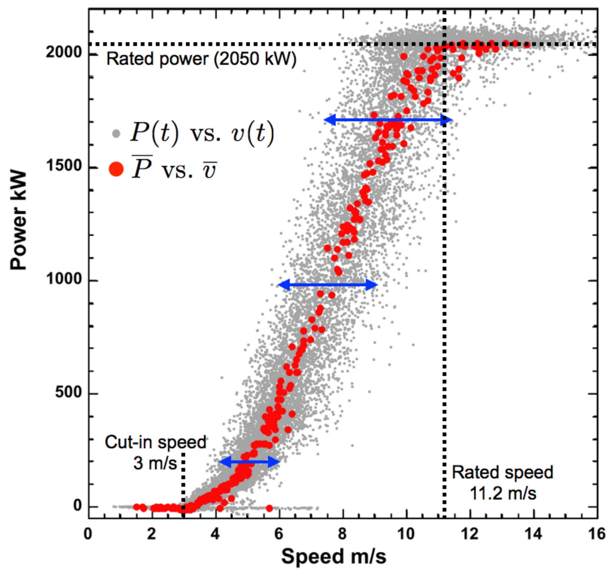
In
Figure 1, we plot the power curve (
vs.
, solid red circles) with the instantaneous power against speed (
vs.
, solid grey circles) overlaid on top of the power curve for a 2.05 MW REPower MM92 turbine (cut-in speed: 3 m/s, rated speed: 11.2 m/s, cut-out speed: 24 m/s, rated power: 2050 kW) located at a wind farm operated by EverPower Wind Holdings in Howard, NY (
Table 1). The solid blue arrows marking the scatter in instantaneous wind speed values at
= 5, 7, and 9 m/s qualitatively demonstrate the monotonic increase in wind speed variability with mean speed; i.e., the case of multiplicative variability.
Before proceeding, we note a nuance concerning the time-average for
and
. IEC standard 61400-12-1 [
3] requires that each value of
and
in the power curve be determined by averaging a 10 min time record (sampled at 1 Hz or higher) of
and
, respectively. This translates to an average over 600 s × 1 Hz = 600 samples—at least—for each time-averaged value in the power curve. Since the Howard data set (see
Table 1) was sampled at 0.2 Hz, a pertinent question to ask is whether 600 s × 0.2 Hz = 120 samples are sufficient to achieve statistical convergence of the mean. We performed a bootstrap protocol [
17] for the Howard time series to generate ten different time series by randomly shuffling values of the originally measured time series for
and
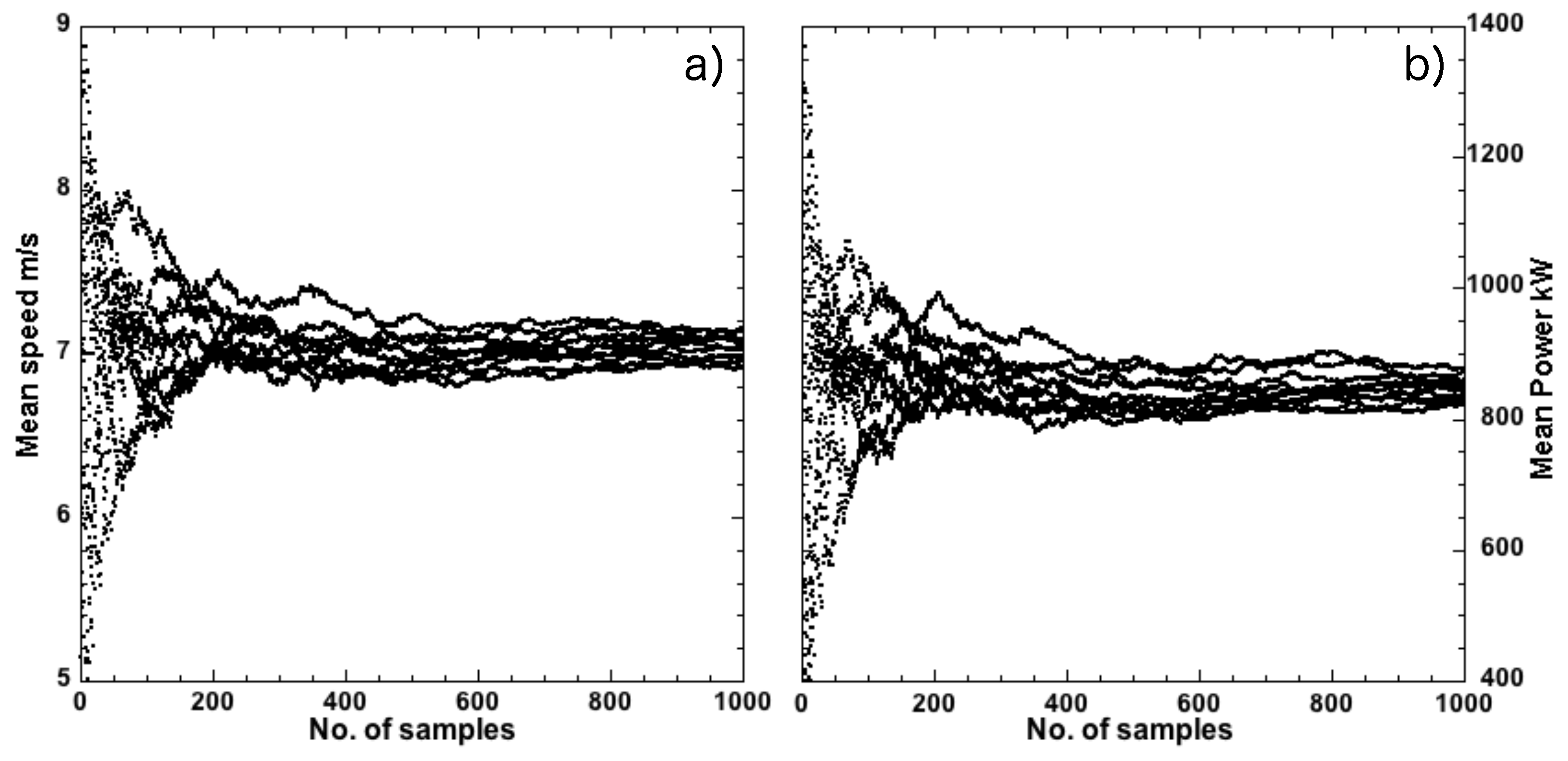
. We then measured the mean for each bootstrap time series as a function of increasing sample size for wind speed and wind power.
Figure 2 shows how the mean wind speed (
Figure 2a) and mean wind power (
Figure 2b) converge as a function of increasing sample size. Since each sample is measured 5 s apart in our data set, 120 samples equate to a 10 min interval prescribed by the IEC standard. As is evident from
Figure 2, asymptotic statistical convergence of the mean values is achieved only at about 400 samples. Following from this statistical convergence test, we constructed the power curve in
Figure 1 by averaging over 400 samples (i.e., a 33.3 min time record for each value of
and
). We emphasise that the bootstrap protocol tests for statistical convergence in the absence of correlations. The successive values in the measured time series are correlated; i.e., the
nth value will lie within a certain band relative to the
th and
th values, depending upon correlation strength and correlation time. When this measured series is randomly shuffled to generate a synthetic series for the bootstrap test, the correlations between successive values in the time series are lost. On the other hand, when using the actual time series for
and
in constructing the power curve from averages, such correlations persist and reveal themselves in the variability, as we discuss below.
3. Results and Discussion
We analysed three data sets (
Table 1), one (Howard) containing both wind speed and wind power time series, and the other two (Big Bear Lake and Atacama) containing only wind speed time series.
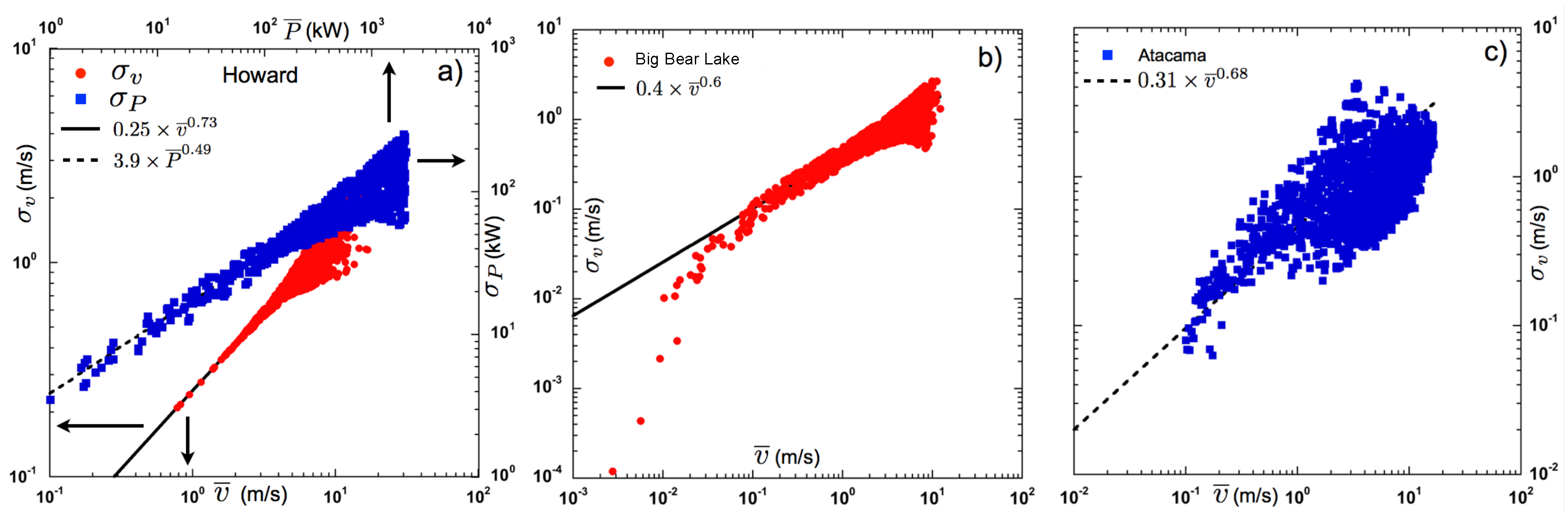
Figure 3a plots the standard deviations of wind speed
and wind power
versus mean wind speed
and wind power
, respectively, for the Howard data set. The standard deviation of wind speed
(solid red circles in
Figure 3a) scales algebraically relative to the mean wind speed
with a power-law fit that follows the form
(solid line in
Figure 3a). The standard deviation of wind power fluctuations
(solid blue squares in
Figure 3a) also exhibits algebraic scaling, albeit shallower than wind speed, with a power-law fit of the form
(dashed line in
Figure 3a). Wind speed standard deviation
for the Big Bear Lake data set plotted in
Figure 3b (red solid circles) exhibits a similar algebraic scaling, but with a different power-law exponent (
, solid black line in
Figure 3b) from the Howard data set. Finally, for the Atacama data set, although
exhibits a systematic increase with
(solid blue squares in
Figure 3c), we find that the scatter is too high to make a conclusive determination of power-law scaling. We do include a power-law fit (dashed line in
Figure 3c), but one should not derive any inferences from this fit. Be that as it may, the fact that
exhibits monotonic increase with
for all data sets establishes the scenario of multiplicative variability.
The observed scaling for power fluctuations (
) is significant given that Calif et al. [
18] have recently reported the same
scaling for a single turbine as well as for wind farms at various planetary locations. They interpreted this scaling within the context of the “Taylor Rule” [
19] (not to be confused with Taylor’s Hypothesis in turbulence theory [
20]), also called “Fluctuation Scaling” [
21] in physics, where the 1/2 scaling exponent forms one of two limiting cases. However, based on additional empirical evidence for wind speed fluctuations and calculations resulting in Equation (
7), we proffer an alternative interpretation for this scaling.
Consider a time-varying signal
with a signal correlation time
. The mean
and standard deviation
become truly time-independent when the average is taken over several multiples of the correlation time
. Instead, if the averaging interval
, residual correlations persist in
and
(subscript
τ now denotes the averaging interval) which vary with averaging time
τ. Wind speed (and therefore wind power) fluctuations which reflect atmospheric turbulence possess long time correlations extending up to 24 h timescales [
22,
23,
24,
25,
26], whereas the IEC standard [
3] specifies a 10 min time average for calculation of
and
. Even our bootstrap protocol specifically tests for statistical convergence in the absence of temporal correlations; generating a new randomised time series from the original time series destroys temporal correlations in the signal. Consequently,
and
retain residual correlations, which are revealed as systematic variation in
relative to
(the same applies to
and
). Such relative scaling between moments of a distribution is well known via Extended Self Similarity (ESS) scaling [
27], and was fruitfully exploited to accurately estimate deviations from scalings predicted by the Kolmogorov theory of turbulence [
28]. Our observed scalings between the mean and standard deviation of wind speed follow in the same spirit. One cannot escape the residual correlations—and hence the power-law relationship between
and
—unless the averaging time is increased from the IEC-stipulated 10 min to the signal correlation time of order 24 h. A 24 h averaging time for each point on the power curve calls for several months worth of data collection effort, and hence is clearly impractical. A more tractable—and still quantitatively defensible—approach is to incorporate the power-law scaling between
and
to self-consistently account for residual correlations in the power curve and its variability, as we show below in Equation (
8).
We can now substitute the scaling form
in Equations (
5) and (
7) to obtain:
Equation (
8) therefore provides a minimal parameter description of
and
as a function of
alone, thereby keeping our analysis in accord with the requirements of IEC standard 61400-12-1 [
3]. Even when a scaling form for
is unavailable (e.g., the Atacama data set), one can still exploit the monotonic variation in
versus
and numerically input
and
into Equation (
7) and calculate
to establish confidence intervals around
for forecast projections. Failing this, the wind speed variability feeds into and amplifies wind power variability, and
transforms into forecast uncertainty.
Equation (
8) applies between the turbine’s cut-in and rated speeds. Furthermore, we emphasize the fact that Equation (
8b) is only a leading order approximation for wind power variability between the cut-in and rated speeds. Between the rated and cut-out speeds, mean power decouples from mean speed, and the turbine acts to rectify wind power fluctuations, thereby suppressing any increase in power variability. When wind power fluctuations are considered as a whole between the cut-in and cut-out speeds,
should follow a shallower scaling than would be suggested by Equation (
8b). Given that the range of speeds between the rated and cut-out speeds is roughly half the entire operating range of wind speeds for any given turbine, it may explain why
seems to hold universally.
It is, however, revealing that the Howard and Big Bear Lake data sets do not share the same scaling exponent
, despite sharing the same averaging duration. This suggests that environmental factors local to the measurement location strongly influence wind dynamics, thereby controlling the value of the scaling exponent
. A clue to this effect is revealed by the strongly anomalous behaviour of the Atacama data set, which does not exhibit as clear a scaling (
Figure 3c) as the other two. The Atacama location (Chajnantor, Chile) differs significantly from Howard and Big Bear Lake in at least two respects. Firstly, Howard, NY and Big Bear Lake, CA are at 605 m and 2085 m elevations, respectively, whereas Chajnantor in Atacama has an elevation of 5080 m above sea level. This strong disparity in elevations translates to difference in air density and wind profiles, which must certainly affect wind speed variability.
Second, Big Bear Lake is adjacent to forested mountain ridges that rise several hundred meters above the lake. The rural farmland in Howard, NY has interspersed forest and cultivated land. On the other hand, the Chajnantor location in the Chilean Andes is a desert. The influence of surface roughness on the atmospheric boundary layer is well known in the environmental sciences, where internal atmospheric boundary layers are associated with the horizontal advection of air across a discontinuity in some surface property [
29]. Identification of the precise environmental factors will require field observations, and cannot be achieved with wind speed data alone; hence, this lies beyond the scope of the current work. Furthermore, the sub-linear power-law scaling of
relative to mean speed
points to the existence of a hidden length scale, either in the atmospheric flow or in the planetary surface roughness. This hidden length scale—if identified through extensive observational measurements—could potentially extend the phenomenology of flow within the shear boundary layer beyond mean wind profiles to include fluctuations. Such a phenomenology would of course mark an advancement in geophysical fluid dynamics, but would also benefit the wind engineering community. High time-resolution wind data sets that extend over several days are few, and are prized by researchers. The generation of such data sets in several locations would be a worthy goal for national research agencies.


