1. Introduction
The photovoltaic electrical energy generation has received a great deal of attention in the last decade, thanks to its zero emission impact, government financed incentives and the zero cost of its primary energy. Indeed, the solar irradiance availability in the planet allows us to get free power once the initial plant investment has been faced [
1]. The scientific community has pointed out several improvable aspects, the efficiency of the photovoitaic (PV) cells being of paramount importance [
2,
3,
4]. As no cost is associated with solar energy availability, the proximity of the PV operating point to its maximum power produces the same results as the PV cells with improved efficiency. In other words, a solar power plant should always be working as close as possible to its maximum potential in terms of power, in order to really exploit any possible improvement in the efficiency of the PV cells. In order to track the PV maximum power point, several strategies have been proposed. The most diffused applications use the
Perturb and Observe technique [
5], where the setting of perturbation step can also be adaptive [
6], and
Incremental Conductance [
7]. Several low level control algorithms have been proposed in tandem with such control strategies [
8,
9]. The overall system efficiency may also depend on whether the Maximum Power Point Tracking (MPPT) is applied with a centralized or distributed approach on the various PV panels [
10]. The last solution is mostly suitable for low power application [
11]. Most of the MPPT techniques require the panel parameter values [
12] and are based on both measurements of PV current and voltage.
Another important aspect is regarding the priority consumption of the green energy production versus traditional production from fossil energy sources, which is also pursued by means of fault-tolerant converters [
13]. This goal can be achieved by means of topology changeable converters [
14,
15], capable of reconfiguring themselves via static switches. A different solution is based on interleaved converter topologies [
16,
17], where the total power is distributed among two or more identical modules. In the case of a fault occurrence on one of the modules, this solution guarantees the continuity of the operation, even if at reduced maximum power.
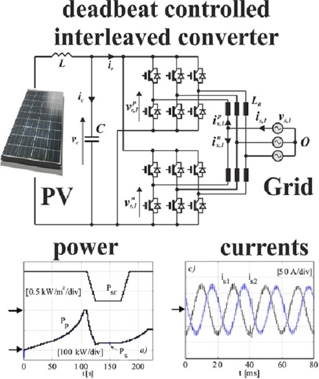
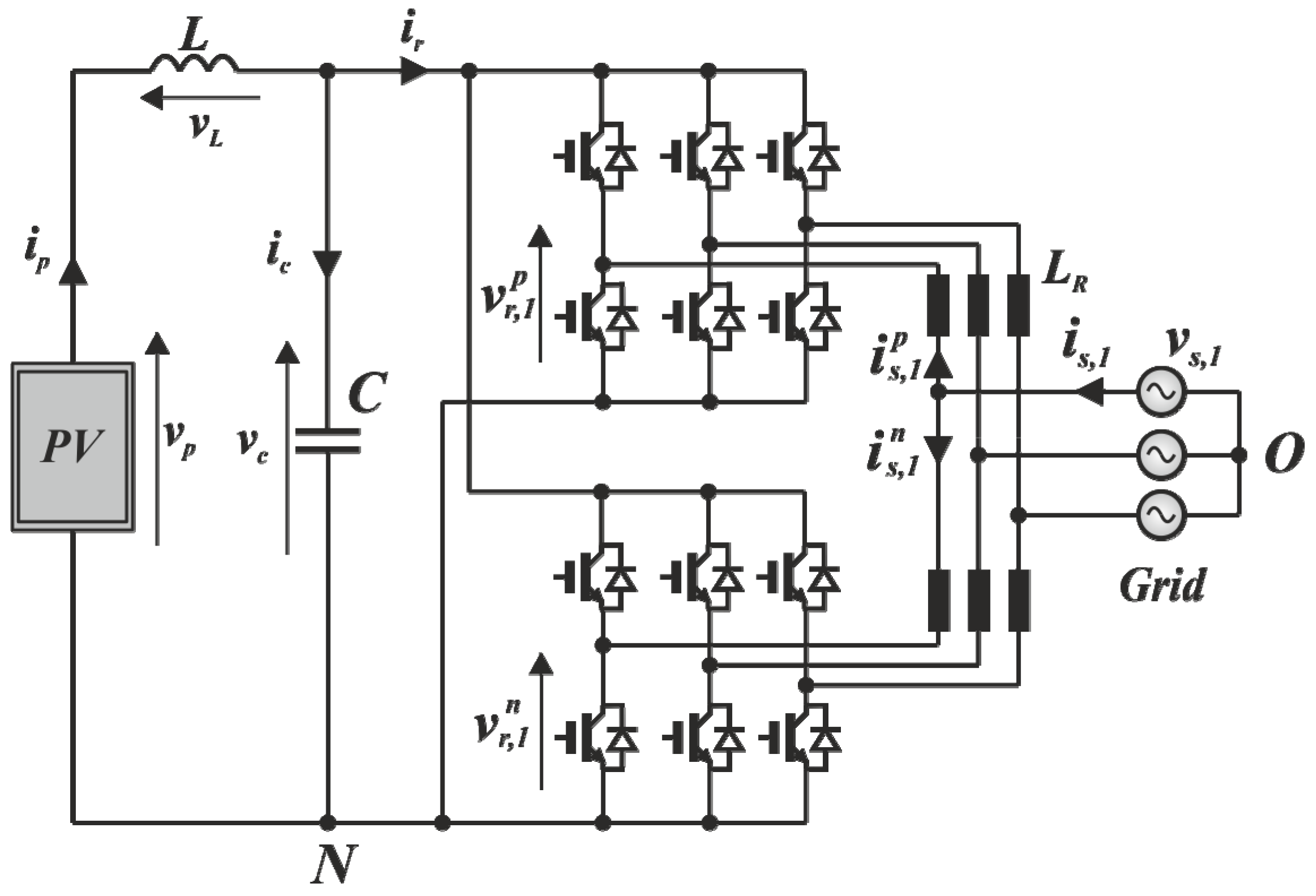
In this paper, a two-channel, three-phase grid connected, interleaved inverter is coupled with a PV array via a LC filter. The proposed tracking algorithm of the PV array is an evolution of the one introduced in [
18,
19] and is applied with a centralized approach in the context of a medium power system (around 200 kW). This strategy requires only one voltage measurement and, as it is based on a hysteresis approach, it ensures a very low power ripple around the PV MPP. The MPPT output is then processed by the inverter control algorithm for which a space vector modulation technique is proposed.
3. The Proposed MPPT Algorithm
The power
PGrid injected by the interlaced converter in the electric grid can be linked easily to the power absorbed from the PV array plus LC filter
PDC by neglecting the Joule or switching the losses of the converters and by imposing that the currents are uniformly distributed between the channels of the interleaved converter:
where the magnetizing power of the circulating inductors has been neglected with respect to the grid power, because, by choosing proper values for the inductance and by taking into account that the current gradients are strongly limited by the considered application, it results in
. From (1), it is clear that the
PDC can be imposed by properly controlling the line currents. Therefore, the system, composed of the controlled interleaved converter plus the electric grid, can be replaced by a controlled current generator for which the current value is linked to
PGrid:
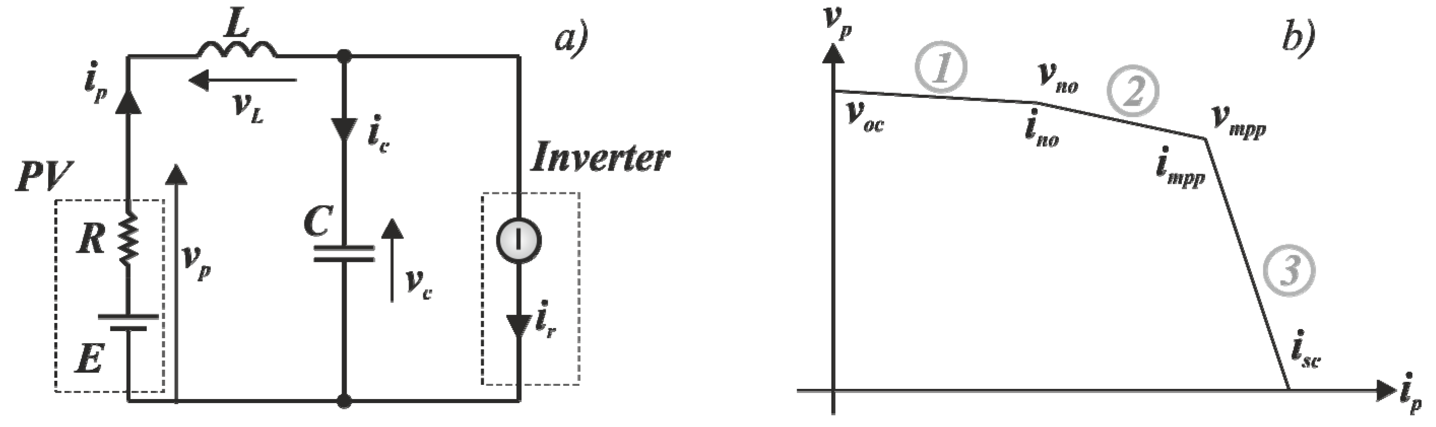
Indeed, in order to discuss the proposed MPPT algorithm in detail, in
Figure 2a, the topology of the system is proposed in a simplified manner. The inverter is substituted by an ideal current generator and the PV array is represented by an ideal voltage generator connected in series with an internal resistance.
The values of
E and
R depend on the actual PV operating point following the characteristic of
Figure 2b. In other words, the real PV characteristic is approximated by a linearization process identifying three different linear laws. The quantities
vmpp and
impp refer to the PV maximum power point, while
voc and
isc are the PV open circuit voltage and the short circuit current respectively.
The MPPT algorithm is based on the capacitance voltage measurements and, in particular, on its time derivative d
vc/d
t. Starting from zero, the power requested by the inverter increases linearly with time with a prefixed slope. The power slope can be fixed such that the system reaches its rated value in a prefixed time (
tStartUp):
As it is seen further, the LC filter is sized such that the inductor voltage drop and the capacitance current absorption are negligible with respect to their rated values and, as a consequence, the PV current and voltage time derivatives only depend on the inverter power slope via the PV characteristic. This ensures that the time derivative of the capacitance voltage is limited to the PV characteristics (see
Figure 2b).
During the time when the requested power linearly increases, the PV operating point of
Figure 2b moves from left toward right. Before the MPP is reached, d
vc/d
t is negative and its absolute value is limited by the zone 2 of the PV characteristic. When the power requested by the inverter gets higher than the MPP, the PV power does not increase any further. Indeed, the inductor keeps the PV current stable to a value very close to the MPP and the PV operating point moves slightly at the right side of MPP. The inverter requested power keeps increasing and the extra power absorption is taken from the capacitor, whose voltage time derivative keeps decreasing as the difference between the inverter current and the PV current keeps increasing.
This phenomenon testifies that the MPP has been reached and is being overcome. Following a symmetrical hysteresis approach, when dvc/dt gets lower than a prefixed negative threshold, the slope of the requested power is inverted so that the time derivative of capacitance voltage starts increasing and the PV operating point moves toward left again, thus, toward the MPP. The slope of the requested power is kept at negative until dvc/dt overcomes the positive threshold and, after that, the requested power slope is inverted again by repeating the process.
In order to facilitate the comprehension of the proposed algorithm, a numerical analysis based on the ideal case of
Figure 2. has been carried out and some results have been proposed in
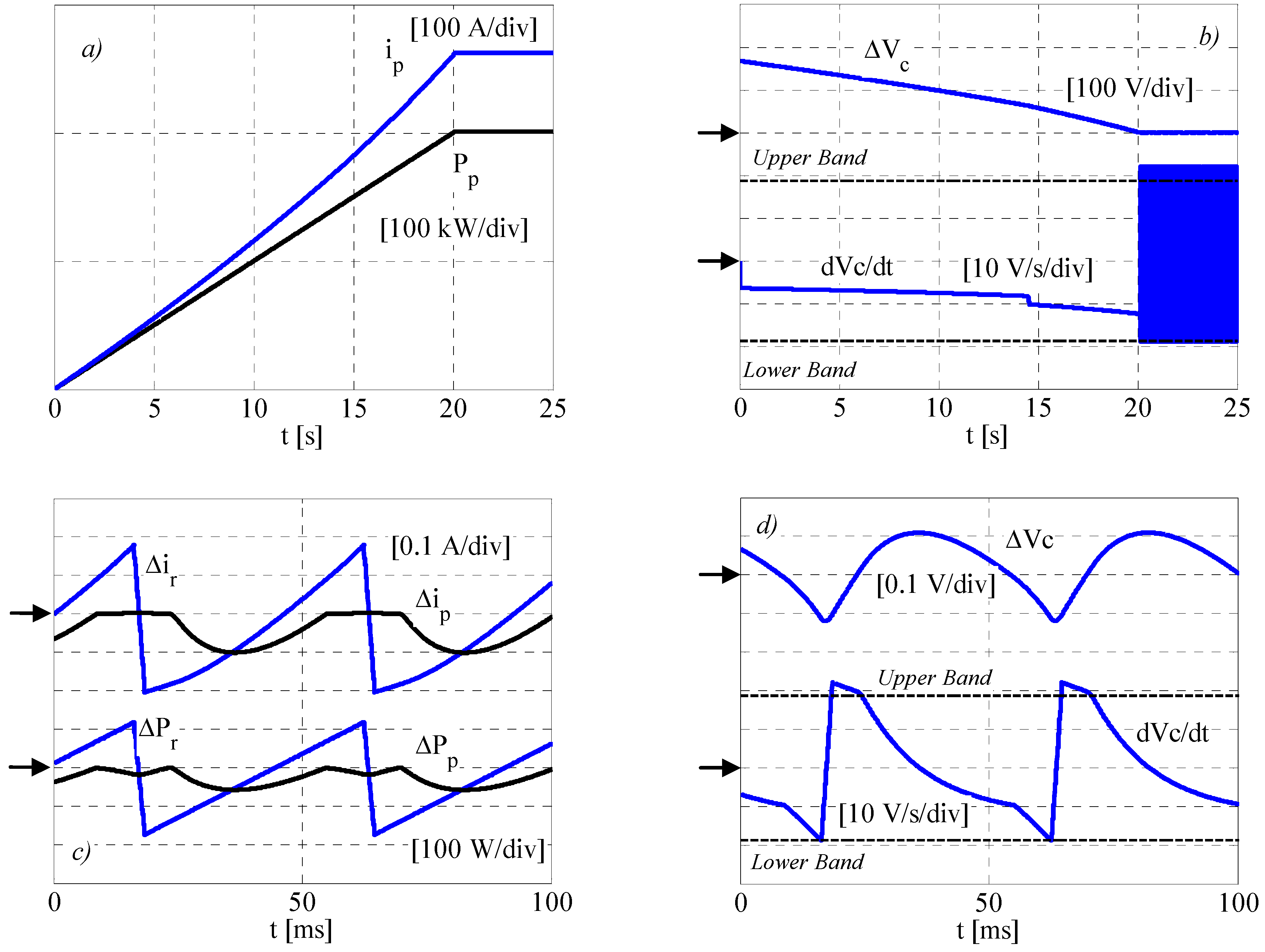
Figure 3.
Figure 3a shows the PV current and power during the startup of the system. The power increases linearly with time, according to the power requested by the inverter, and, as the
vc variation is small, the current also has an almost linear behavior. In a time span of about 20 s, they reach their respective rated values and the system can then be considered in steady state conditions. In
Figure 3b, two quantities are reported: the time derivative of the capacitor voltage, and its variation with respect to the rated value. As it can be noted, while in the startup interval, the quantity d
vc/d
t is well within the hysteresis threshold; in the steady state condition, the hysteresis controller is activated and thus,
vc is constrained to its rated value.
In
Figure 3c, the PV power and current variation with respect to their rated values are reported and compared to the same quantities as the inverter. The variable requested by the inverter is denoted with the subscript
r, while
p refers to PV quantities. As it can be noted, after the MPP is reached and during the positive slope of the requested power, the
ip current and the
Pp power remain almost constant and their values correspond to the PV MPP. The same can be said during the negative slope of the requested power. When the
vc derivative touches its negative threshold, the requested power slope gets positive again and the PV quantities slightly vary until the MPP is reached again. The total variation of
Pp and
ip is very low in comparison to the rated values.
In
Figure 3d, d
vc/d
t and Δ
vc waveform are consistent with the behavior of the controlled system and they testify the low ripple of the capacitor voltage.
3.1. Voltage Derivative Threshold
The symmetrical hysteresis control threshold for the capacitance time derivative has to be chosen such that before the MPP (left side of MPP on
Figure 2b); the chosen positive slope of the power requested by the inverter causes a value of d
vc/d
t within the band, while after the MPP (right side of MPP on
Figure 2b), d
vc/d
t overcomes the band. The expected value of d
vc/d
t at the left side of MPP can be easily calculated assuming a low ripple on the capacitance voltage. In this case, indeed, the slope of the inverter current is proportional to the slope of power (via the reciprocal of
vmpp). As the filter is sized such that the PV follows the request of the inverter, the time derivative of the PV current corresponds to the one of the inverter, and the time derivative of the capacitance voltage corresponds to that of the PV array. Thus, the expected time derivative of the capacitance voltage can be written as follows:
with
R2 = –d
vp/d
ip belonging to the second zone of the PV characteristic of
Figure 2b.
Using a safety coefficient of 2, a reasonable value for the hysteresis band can be chosen as follows:
3.2. Filter Sizing
In order to ensure that inductor voltage drop and the capacitance current absorption are negligible with respect to their rated values, the maximum values of
L and
C can be found by Equation (6):
In the series
R,
L,
C of
Figure 2a, it is easy to verify that the PV current is characterized by a damping factor whose expression is:
In order to ensure that the variation of the PV current is low, the damping factor must assume a high value (ζ >> 1). On the other hand, it has to be remembered that, in contrast to the ideal examined case, the real converter will introduce a high harmonic content linked to the chosen switching frequency. This harmonic content will reflect on the PV current via a reduction factor
ξr depending on the chosen
L and
C values.
In order to ensure that the PV operating point is kept very close to the MPP, the reduction factor must be fixed at a high value. Setting minimum values for the damping factor and the reduction factor, the following conditions have to be satisfied:
3.3. Negative Power Slope
The value of the negative requested power slope must be chosen in order to ensure the rapid recovery of the MPP, after it has been overcome during the positive slope, and keeping the capacitor voltage variation within a reasonable value. The circuit of
Figure 2a can be considered for the calculation of the capacitor voltage, assuming that the PV current is held to the MPP value by the inductor presence. As the
vc variation is expected to be very low, the following law can be assumed for the
ir current:
Solving the first-order differential equation, the
vc variation results as follows:
By limiting the maximum
vc variation, it results as follows:
3.4. Chosen Values
The chosen values for the startup time and for the limits of Equations (6), (9), and (13) are summarized in
Table 1, together with the chosen values of the filter inductance and capacitance and the requested positive and negative power slope.
Finally, it has to be noted that the sizing procedure has been illustrated with reference to the standard irradiation (1 kW/m2) and by fixing strong constraints. If referred to partial shading conditions; the same procedure would have led to different values of chosen parameters. Thus, in the real case of variable irradiation, the fixed limits may not be fulfilled by the chosen parameters. Nevertheless, as it will be seen in §6, the chosen values will continue to assure satisfying results, even for a deep shading condition.
Indeed, the only parameter that should be fine-tuned across the whole range of the operating conditions is the positive reference power slope. In fact, in contrast to the ideal case of
Figure 3—carried in the standard condition—the value of the hysteresis threshold is linked to the positive power slope and the PV voltage derivative in correspondence to the MPP:
From Equation (14), it can be seen that
should be changed as a function of radiation on which
depends. However, a variation of
would lead to variable behavior of the PV power ripple across different operating conditions. Instead of fixing the
constant, an adaptive law of
pslope is proposed, which is as follows:
In Equation (15), the voltage derivative depends on the actual PV developable maximum power. If any instantaneous assigned reference power value
P* is considered to be equal to the PV developable maximum power,
will depend on the actual assigned power via the PV characteristic. Thus, the power slope is a time-dependent function:
The power slope will be assigned depending on the actual power value in the further numerical analysis (§6), where the ideal generator is replaced by the real inverter and shading conditions are investigated. This will result in an increase in the startup time. However, the system will reach its rated power in a reasonable time value of about 110 s.
4. Interleaved Inverter
4.1. Mathematical Model
With reference to
Figure 1, as already pointed out, the inverter is composed of two identical three-phase half bridges. Each of the two modules is a converter itself, and the superscripts
p and
n are used respectively for the upper and lower ones. For clarity, in
Figure 1, only the first phase voltages and currents are indicated. For the generic
kth phase, the following voltage balance can be written as follows:
where
is the voltage of the point,
N referred to the grid neutral point
O.
Referring to the same index
k, the semi-sum of the first and second of Equation (17) gives the following:
The space vectors
y can now be introduced, together with the homopolar components
y0, by means of the following transformation:
The Equation (18) can then be written as follows:
The first of Equation (18) gives the grid current space vector behavior as a function of the two converters’ space vector voltages, while the second establishes that the neutral point displacement voltage instantaneously coincides with the semi-sum of the two converter homopolar voltages .
Referring to the same index
k, the difference of the first and second of Equation (17) gives the following:
The two converters’ phase currents can be expressed as follows:
with
as the common mode current on the
kth phase of the interleaved inverter, Equation (21) can be rewritten as follows:
Applying the transformation of Equation (19):
Finally, the interleaved inverter mathematical model is given as follows:
It is now clear that the inductors LR are necessary to filter the harmonic content, which is introduced by the modulation of vr, limiting the oscillation on the grid currents. Moreover, their presence makes the common mode currents controllable, keeping their rising/falling time at values that are suitable to the control algorithm sampling time.
4.2. Control Strategy
Once the reference power is available by means of the already discussed MPPT algorithm, the control strategy of the inverter is responsible for assuring that this power is drained only by the fundamental direct component of the grid voltages.
Decomposing the grid voltage space vector into its harmonics is shown as follows:
The reference space vector current has to satisfy the following:
The quantities and are estimated by means of a Phase-Locked Loop algorithm (PLL).
From the grid’s current reference
, it is possible to determine the converter space vector reference voltage
by means of a
minimum delay deadbeat control algorithm. Denoting the sampling time interval with
Ts and the generic sampling time instant with
tm, the algorithm is based on the following equation:
As the grid voltages are repetitive, in a steady state condition the prediction of the voltage grid space vector can be estimated by memorizing the values into a circular buffer; the minimum buffer size must be one period of . Sudden perturbations of the grid voltage can be easily identified by comparing the sampled value with the expected one. In this case, the prediction can only be based on the most recent sample, i.e., .
The total interleaved inverter space vector reference voltage value can be derived from Equation (28), which, according to Equation (25), is the semi-sum of the
p and
n converters’ space vector reference voltages. In order to separately calculate the references for the upper and lower half bridges’ converters, an optimum condition has to be added. In an ideal case, the common mode currents would be null in all the three phases:
The differential voltage components can again be calculated by means of a deadbeat control:
Based on the position in Equation (25), the reference space vector voltages for the two converters can be evaluated:
4.3. Modulation
In each sampling time (tm+1, tm+2) the voltages and can be obtained by a synchronous space vector modulation using a triangular carrier of a proper frequency value. The switching frequency can be fixed either equal to the sampling frequency or half of the sampling frequency. Denoting with Tm the modulation period and Ts the sampling time, it will be Tm = Ts or Tm = 2 Ts. Furthermore, it is advantageous to fix a phase shift between the upper and lower converter triangular carrier. Indeed, by choosing this phase shift correspondent to the half of Tm, the main voltage harmonic, due to the modulation, will be null on the total interleaved inverter voltage space vector.
In each modulation period, the space vector modulation pattern applies four vectors, as follows:
The vectors
,
correspond to null vectors 1-1-1 and 0-0-0, applied with duty cycle
and
respectively, while
and
are active vectors, applied with duty cycle
and
respectively. The duty cycles of active vectors are fixed by the space vector reference values and their sum is related to the null vectors’ duty cycles by the following condition:
Thus, one degree of freedom remains in order to establish the value of all duty cycles. It can be exploited to control the homopolar component
. For each of the two converters, the null vectors duty cycles
,
can be expressed as a function of a correction factor
:
Setting
, the homopolar components of vectors
and
will be expressed as follows:
The semi-difference of the two equations in Equation (35) gives:
where,
is the component of
, which is invariant with
. In particular,
when
. By imposing
,
is then computed as follows:
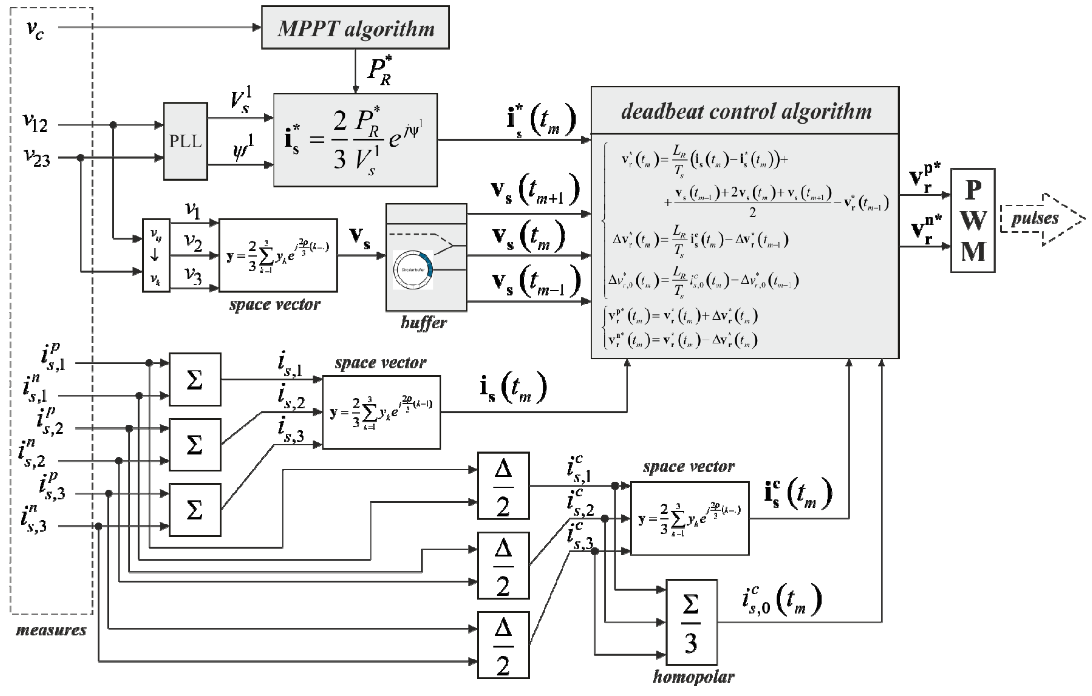
5. Control Algorithm and Numerical Analysis
In
Figure 4, the total system control diagram is reported consistently with the technique discussed in the previous paragraphs.
As the measurement of the capacitor voltage is influenced by the modulation and contains oscillations linked to the switching frequency, a low pass filter is implemented for the processing of vc. This additional signal processing is needed in order to avoid false detections of hysteresis thresholds crossing.
The control strategy of the proposed system has been tested by performing an extensive numerical analysis in the Matlab Simulink ™ environment. The parameters’ values used in the simulation are reported in
Table 2.
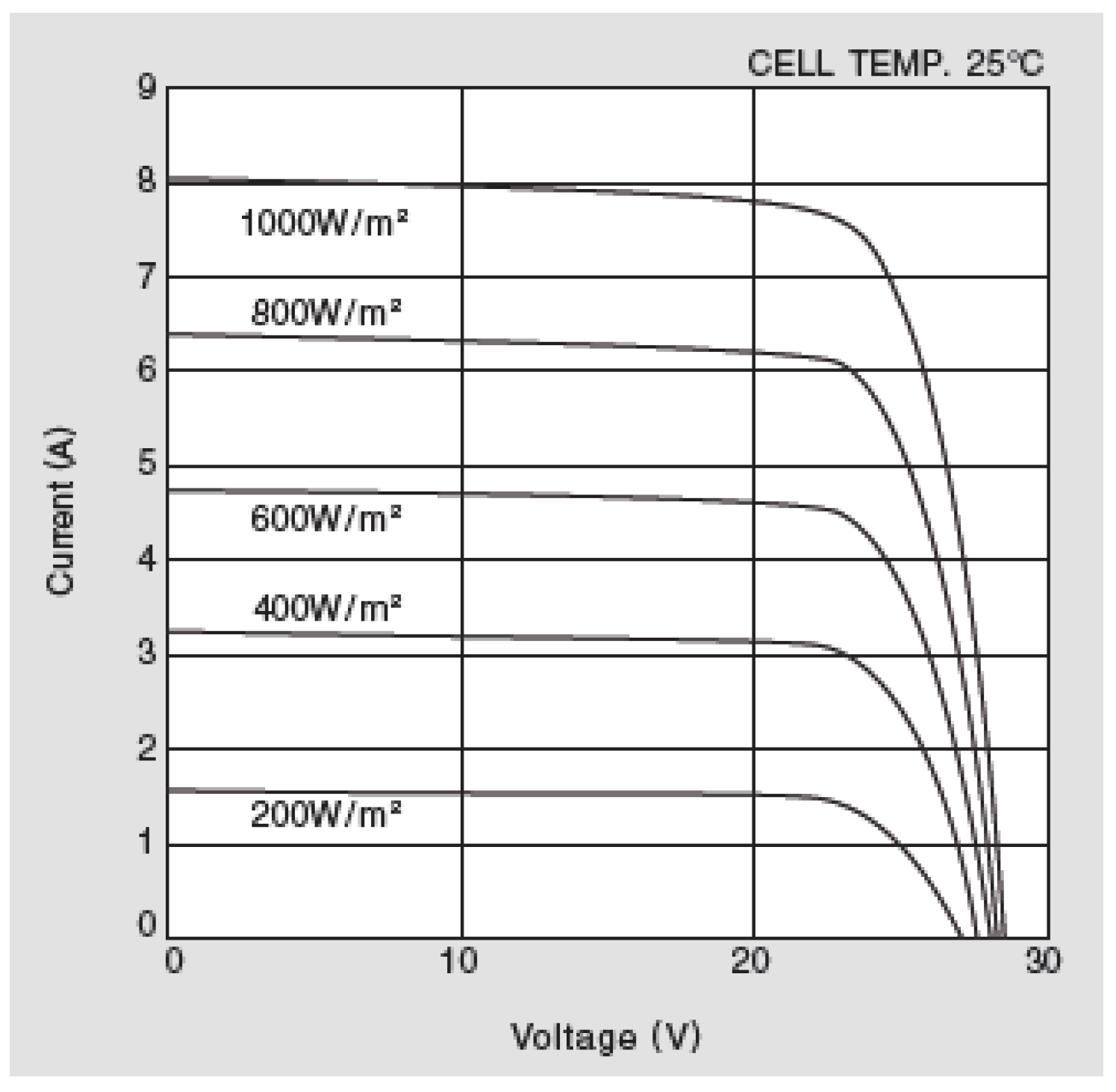
In this context, the ideal voltage/current characteristic of the PV array has been replaced by a real one based on the commercial multicrystal modules: KIOCERA KC175GHT-2 (see
Figure 5). Moreover, a detailed dynamic model of the chosen IGBTs has been implemented (SEMIKRON SKM400GB176D).
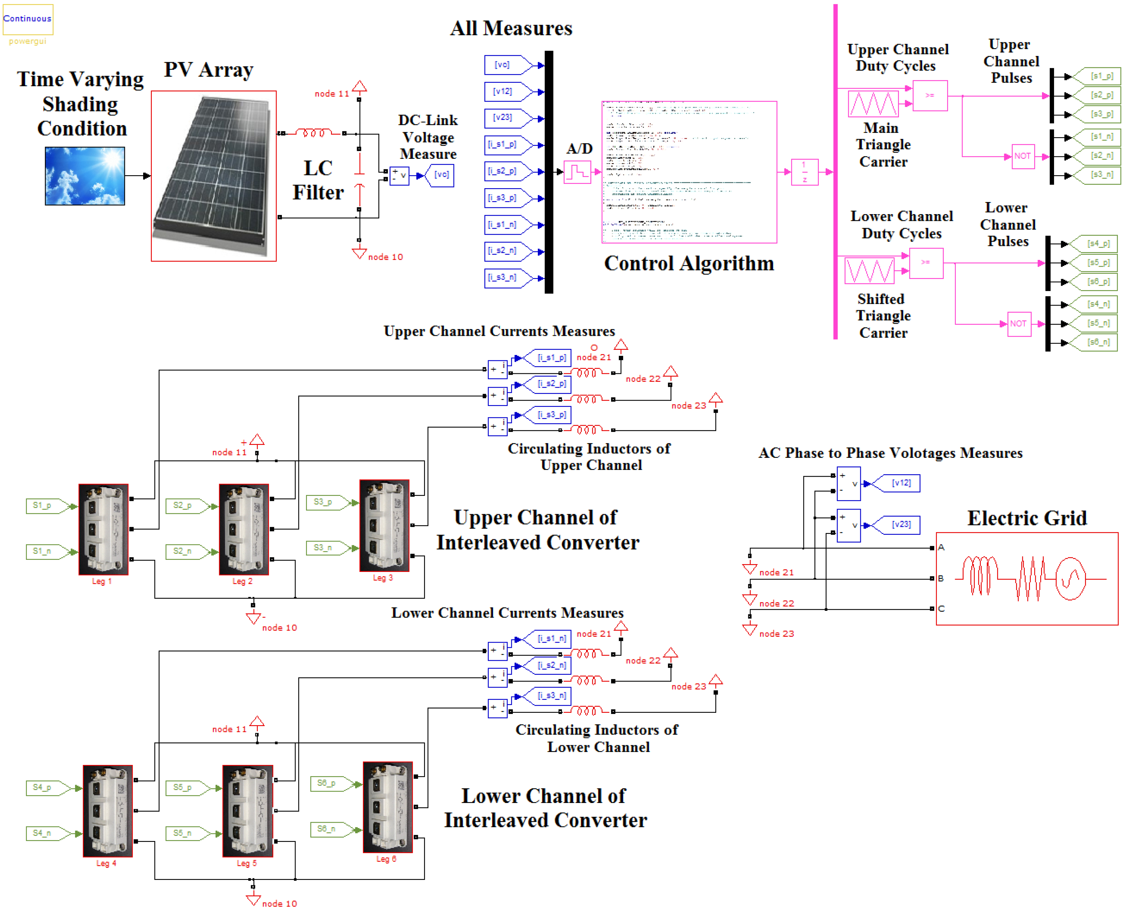
The Simulink model of the whole controlled system is reported in
Figure 6, where it is possible to distinguish between four main sections: the PV array, the interleaved converter, the electric grid, and the control algorithm. Except for the electric grid, for which a standard Simulink block has been used, the other subsystems have been implemented by means of C-language S-Functions. In particular, for the models of the PV cells and forthe IGBTs, continuous states of S-Functions have been used, while the control algorithm has been implemented as a discrete S-Function, which is computed at the sampling rate of 200 µs.
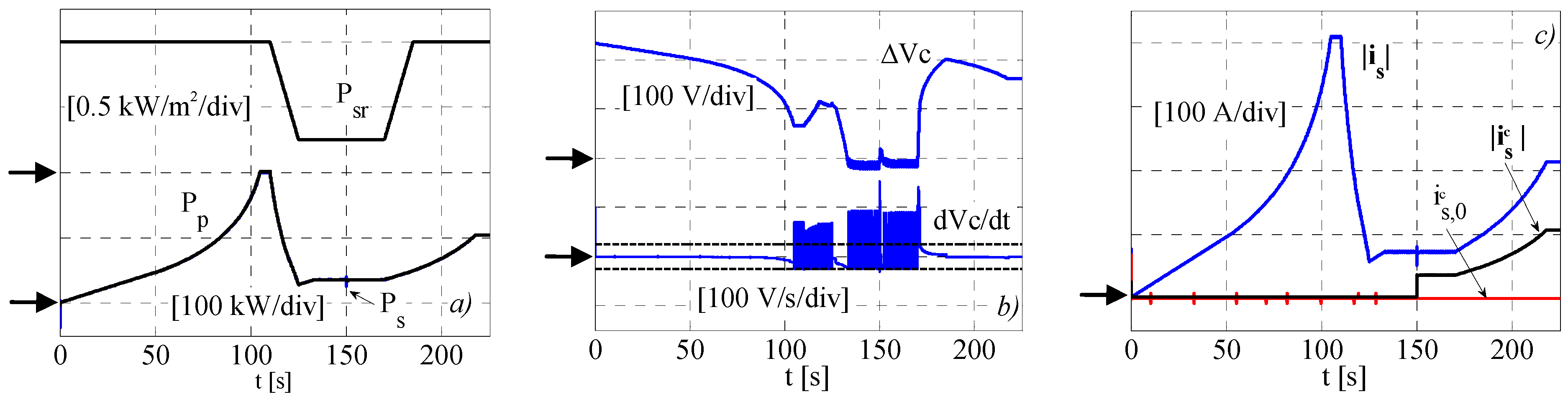
The whole time window simulation results are reported in
Figure 7. The simulation interval (225 s) can be split into four sub-intervals, which are as follows:
With a solar radiance kept constant at 1000 W/m2, the control of the converter is activated at t = 0.
At t = 110 s, the solar radiance starts decreasing linearly with a slope of 50 W/m2s−1, until it reaches 250 W/m2.
At t = 150 s, a fault occurs in the lower module of the two channel interleaved converter.
At t = 170 s, the solar radiance starts increasing linearly with a slope of 50 W/m2s−1, until it reaches 1000 W/m2
Figure 7a shows the PV power
Pp, the grid power
Ps, and the solar radiation
Psr in the whole time range of the numerical analysis. It can be seen that the PV power follows the MPP with good transient behavior, either in correspondence of the standard condition (1000 W/m
2) or during the fast varying shading conditions. After the fault event, the grid power
Ps remains practically constant, except for a really quick transient induced by the dynamic of the operating converter, whose currents have to compensate for the faulted one. Finally, when the solar radiation starts to increase, the steady state condition is reached at a value of power that is lower than the MPP, as the power limit has been activated on the remaining converter.
In
Figure 7b, the capacitor voltage variation with respect to 700 V is shown (
), together with the capacitor voltage time derivatives. It can be noted that the capacitor voltage, kept practically constant in the steady states conditions, indeed increases during the first transient. This is due to the time response of the PV MPPT algorithm, which induces an average positive voltage derivative in the DC-Link capacitor when the solar radiance rapidly decreases.
Finally, in
Figure 7c, the space vector module of grid current and common mode converter current is reported, together with the common mode homopolar component. It can be noted that, before the fault occurring event, the common mode currents are kept at very small values (<0.1%). As expected, after the fault event, the module of the space vector associated with the common mode current simply coincides with half of the remaining converter one (see Equation (22)), while the correspondent homopolar component is null. The module of the line currents space vector is practically constant in the steady state condition, i.e., a low ripple is induced in the line currents by the proposed MPPT algorithm.
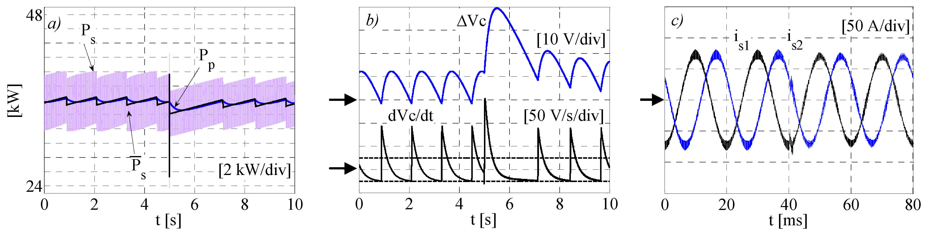
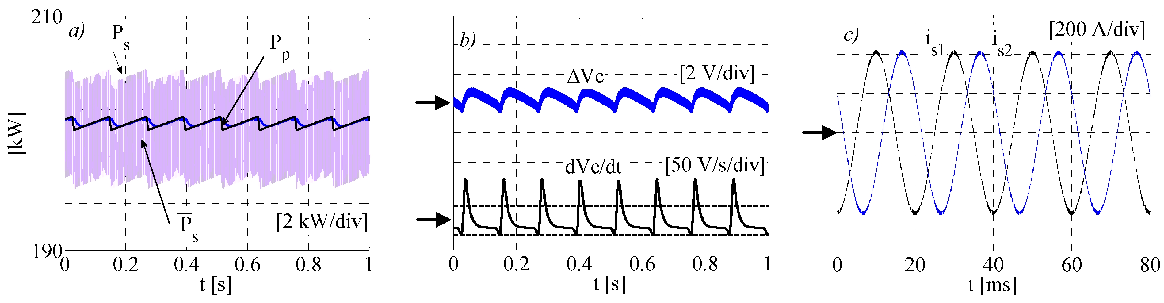
With reference to the steady state condition at 1000 W/m
2,
Figure 8a shows the PV and the grid instantaneous active power together with the grid power, averaged across one modulation period
. The power ripple induced by the MPPT algorithm on the PV power is very small (around 1.1 kW), while the grid power ripple due to the modulation is practically completely filtered out by the LC.
The capacitor voltage variation with respect to
(
) is shown in
Figure 8b, together with the time derivative of the capacitor voltage. While the voltage ripple is kept really low (<0.3 %), the time derivative is not kept within the upper hysteresis band. This is due to the delay introduced by the digital low pass filter on the capacitor voltage measurement. The overall effect is an asymmetrical hysteresis equivalent controller, which produces a voltage ripple higher than the one obtained in the ideal case. Finally, two line currents are depicted in
Figure 8c. As expected, the line currents are sinusoidal and symmetrical; in particular, there is no appreciable oscillation caused by the MPPT.
The same quantities of
Figure 8 are reported in
Figure 9 with reference to the shading condition (250 W/m
2). The behaviors are time centered on the fault event instant. The PV power ripple in steady state conditions is practically equal to the previous case (around 1.1 kW); this testifies the effectiveness of the proposed power slope adaptive control. As expected, the capacitor voltage ripple is instead increased. Indeed, the reduction of the power slope widens the PV power period of repetition and the capacitor filtering behavior becomes less effective. The line currents appear sinusoidal and symmetrical, even after the fault event. At the time instant of the converter failure, the remaining operating converter is able to quickly compensate for the missing channel. Indeed, the line currents are a little affected (see
Figure 9c). Nevertheless, an evident power grid spike is present at the fault instant. In the presence of this perturbation, the MPPT is able to quickly recover the previous operating point (
Figure 9a,b).
6. Conclusions
In this work, a control strategy for a two-channel three-phase grid connected inverter, fed by a PV array, has been presented. This topology has been chosen for its intrinsic fault-tolerant features, a paramount aspect in the context of a centralized PV generation system.
The work focuses on two central issues; the first is regarding the MPPT algorithm, and the second is regarding the control of the interleaved converter. In contrast to the most diffused MPPTs, the one proposed needs only one voltage measurement and is based on a hysteresis approach, which guarantees a continuous tracking of the MPP. This MPPT has been coupled with a converter control strategy based on a specific space vector modulation with homopolar component control.
The numerical results, carried out for a 200 kW case study, highlighted the favorable aspects of the proposed techniques. In particular, the MPPT guarantees a very low power ripple in the steady state conditions, while it shows good transient performance even in the presence of strong perturbations, i.e., fast varying shading conditions and converter failure events. The converter is able to follow the reference power generated by the MPPT with negligible errors, ensuring symmetrical and sinusoidal line currents in steady state conditions. The good dynamic performance of the proposed control is further validated by an induced failure of one channel, from which the system is able to quickly recover.


