Determination of Optimal Initial Weights of an Artificial Neural Network by Using the Harmony Search Algorithm: Application to Breakwater Armor Stones

Abstract

In this study, an artificial neural network (ANN) model is developed to predict the stability number of breakwater armor stones based on the experimental data reported by Van der Meer in 1988. The harmony search (HS) algorithm is used to determine the near-global optimal initial weights in the training of the model. The stratified sampling is used to sample the training data. A total of 25 HS-ANN hybrid models are tested with different combinations of HS algorithm parameters. The HS-ANN models are compared with the conventional ANN model, which uses a Monte Carlo simulation to determine the initial weights. Each model is run 50 times and the statistical analyses are conducted for the model results. The present models using stratified sampling are shown to be more accurate than those of previous studies. The statistical analyses for the model results show that the HS-ANN model with proper values of HS algorithm parameters can give much better and more stable prediction than the conventional ANN model.

1. Introduction

Artificial neural network (ANN) models have been widely used for prediction and forecast in various areas including finance, medicine, power generation, water resources and environmental sciences. Although the basic concept of artificial neurons was first proposed in 1943 [1], applications of ANNs have blossomed after the introduction of the back-propagation (BP) training algorithm for feedforward ANNs in 1986 [2], and the explosion in the capabilities of computers accelerated the employment of ANNs. The ANN models have also been used in various coastal and nearshore research [3,4,5,6,7,8,9,10].

An ANN model is a data-driven model aiming to mimic the systematic relationship between input and output data by training the network based on a large amount of data [11]. It is composed of the information-processing units called neurons, which are fully connected with different weights indicating the strength of the relationships between input and output data. Biases are also necessary to increase or decrease the net input of the neurons [12]. With the randomly selected initial weights and biases, the neural network cannot accurately estimate the required output. Therefore, the weights and biases are continuously modified by the so-called training so that the difference between the model output and target (observed) value becomes small. To train the network, the error function is defined as the sum of the squares of the differences. To minimize the error function, the BP training approach generally uses a gradient descent algorithm [11]. However, it can give a local minimum value of the error function as shown in Figure 1, and it is sensitive to the initial weights and biases. In other words, the gradient descent method is prone to giving a local minimum or maximum value [13,14]. If the initial weights and biases are fortunately selected to be close to the values that give the global minimum of the error function, the global minimum would be found by the gradient method. On the other hand, as expected in most cases, if they are selected to be far from the optimal values as shown by ‘Start’ in Figure 1, the final destination would be the local minimum that is marked by ‘End’ in the figure. As a consequence of local minimization, most ANNs provide erroneous results.

To find the optimal initial weights and biases that lead into the global minimum of the error function, a Monte-Carlo simulation is often used, which, however, takes a long computation time. Moreover, even if we find the global optimal weights and biases by the simulation, they cannot be reproduced by the general users of the ANN model. Research has been performed to reveal and overcome the problem of local minimization in the ANN model. Kolen and Pollack [15] demonstrated that the BP training algorithm has large dependency on the initial weights by performing a Monte Carlo simulation. Yam and Chow [16] proposed an algorithm based on least-squares methods to determine the optimal initial weights, showing that the algorithm can reduce the model’s dependency on the initial weights. Recently, genetic algorithms have been applied to find the optimal initial weights of ANNs and to improve the model accuracy [17,18,19]. Ensemble methods have also been implemented to enhance the accuracy of the model. They are also shown to overcome the dependency of the ANN model not only on the initial weights but also on training algorithms and data structure [20,21,22,23].

In this study, we employ the harmony search (HS) algorithm to find the near-global optimal initial weights of ANNs. It is a music-based metaheuristic optimization algorithm developed by Geem et al. [24] and has been applied to many different optimization problems such as function optimization, design of water distribution networks, engineering optimization, groundwater modeling, model parameter calibration, etc. The structure of the HS algorithm is much simpler than other metaheuristic algorithms. In addition, the intensification procedure conducted by the HS algorithm encourages speeding up the convergence by exploiting the history and experience in the search process. Thus, the HS algorithm in this study is expected to efficiently find the near-global optimal initial weights of the ANN. We develop an HS-ANN hybrid model to predict the stability number of armor stones of a rubble mound structure, for which a great amount of experimental data is available and thus several pieces of research using ANN models have been performed previously. The developed HS-ANN model is compared with the conventional ANN model without the HS algorithm in terms of the capability to find the global minimum of an error function. In the following section, previous studies for estimation of stability number are described; then, the HS-ANN model is developed in Section 3; the performance of the developed model is described in Section 4; and, finally, major conclusions are drawn in Section 5.

2. Previous Studies for Estimation of Stability Number

A breakwater is a port structure that is constructed to provide a calm basin for ships and to protect port facilities from rough seas. It is also used to protect the port area from intrusion of littoral drift. There are two basic types of breakwater: rubble mound breakwater and vertical breakwater. The cross section of a typical rubble mound breakwater is illustrated in Figure 2. To protect the rubble mound structure from severe erosion due to wave attack, an armor layer is placed on the seaward side of the structure. The stability of the armor units is measured by a dimensionless number, so-called stability number, which is defined as

$$N_s\equiv \frac{H_s}{\Delta D_{n50}},$$

(1)

where $H_s$ is the significant wave height in front of the structure, $\Delta ={\mathsf{\rho }}_s/{\mathsf{\rho }}_w-1$ is the relative mass density, ${\mathsf{\rho }}_s$ and ${\mathsf{\rho }}_w$ are the mass densities of armor unit and water, respectively, and $D_{n50}$ is the nominal size of the armor unit. As shown in Equation (1), the stability number is defined as the ratio of the significant wave height to the size of armor units. A larger stability number, therefore, signifies that the armor unit with that size is stable against higher waves, that is, the larger the stability number, the more stable the armor units against waves.

To estimate the stability number, it is required to determine the relationship between the stability number and other variables which would describe the characteristics of waves and structure. Hudson [25] proposed an empirical formula:

$$N_s={(K_D\cot \mathsf{\alpha })}^{1/3},$$

(2)

where $\mathsf{\alpha }$ is the angle of structure slope measured from horizontal, and $K_D$ is the stability coefficient which depends on the shape of the armor unit, the location at the structure (i.e., trunk or head), placement method, and whether the structure is subject to breaking wave or non-breaking wave. The Hudson formula is simple, but it has been found to have a lot of shortcomings.

To solve the problems of the Hudson formula, Van der Meer [26] conducted an extensive series of experiments including the parameters which have significant effects on armor stability. Based on the experimental data, empirical formulas were proposed by Van der Meer [26,27] as follows:

$$N_s=\frac{1}{\sqrt{{\mathsf{\xi }}_m}}\left[6.2P^{0.18}{\left(\frac{S}{\sqrt{N_w}}\right)}^{0.2}\right]\text{ for }{\mathsf{\xi }}_m<{\mathsf{\xi }}_c,$$

(3a)

$$N_s=1.0P^{-0.13}{\left(\frac{S}{\sqrt{N_w}}\right)}^{0.2}\sqrt{\cot \mathsf{\alpha }}{{\mathsf{\xi }}_m}^P\text{ for }{\mathsf{\xi }}_m\ge {\mathsf{\xi }}_c,$$

(3b)

where ${\mathsf{\xi }}_m=\tan \mathsf{\alpha }/\sqrt{2\mathsf{\pi }{H}_s/g{T_m}^2}$ is the surf similarity parameter based on the average wave period, $T_m$, ${\mathsf{\xi }}_c={\left(6.2P^{0.31}\sqrt{\tan \mathsf{\alpha }}\right)}^{1/\left(P+0.5\right)}$ is the critical surf similarity parameter indicating the transition from plunging waves to surging waves, $P$ is the permeability of the core of the structure, $N_w$ is the number of waves during a storm, and $S=A/D_{n50}^2$ (where $A$ is the eroded cross-sectional area of the armor layer) is the damage level which is given depending on the degree of damage, e.g., onset of damage or failure.

On the other hand, with the developments in machine learning, various data-driven models have been developed based on the experimental data of Van der Meer [26]. A brief summary is given here only for the ANN models. Mase et al. [3] constructed an ANN by using randomly selected 100 experimental data of Van der Meer [26] for training the network. The total number of experimental data excluding the data of low-crested structures was 579. In the test of the ANN, they additionally used the 30 data of Smith et al. [28]. They employed six input variables: $P$, $N_w$, $S$, ${\mathsf{\xi }}_m$, $h/H_s$, and the spectral shape parameter $SS$, where $h$ is the water depth in front of the structure. Kim and Park [6] followed the approach of Mase et al. [3] except that they used 641 data including low-crested structures. Since, in general, the predictive ability of an ANN is improved as the dimension of input variables increases, they split the surf similarity parameter into structure slope and wave steepness, and the wave steepness further into wave height and period. Note that the surf similarity parameter ${\mathsf{\xi }}_m$ consists of structure slope, wave height and period as shown in its definition below Equation (3), where $H_s/L_m=H_s/(g{T}_m^2/2\mathsf{\pi })$ is the wave steepness. They showed that the ANN gives better performance as the input dimension is increased. On the other hand, Balas et al. [9] used principal component analysis (PCA) based on 554 data of Van der Meer [26] to develop hybrid ANN models. They created four different models by reducing the data from 544 to 166 by using PCA or by using the principal components as the input variables of the ANN.

Table 1. Correlation coefficients of different empirical formula or ANN models.

Author	Correlation Coefficient	Number of Data	Remarks
Van der Meer [27]	0.92 (Mase et al. [3])	579	Empirical formula, Equation (3) in this paper
Mase et al. [3]	0.91	609	Including data of Smith et al. [28]
Kim and Park [6]	0.902 to 0.952	641	Including data of low-crested structures
Balas et al. [9]	0.906 to 0.936	554	ANN-PCA hybrid models

shows the correlation coefficients of previous studies, which will be compared with those of the present study later.

3. Development of an HS-ANN Hybrid Model

3.1. Sampling of Training Data of ANN Model

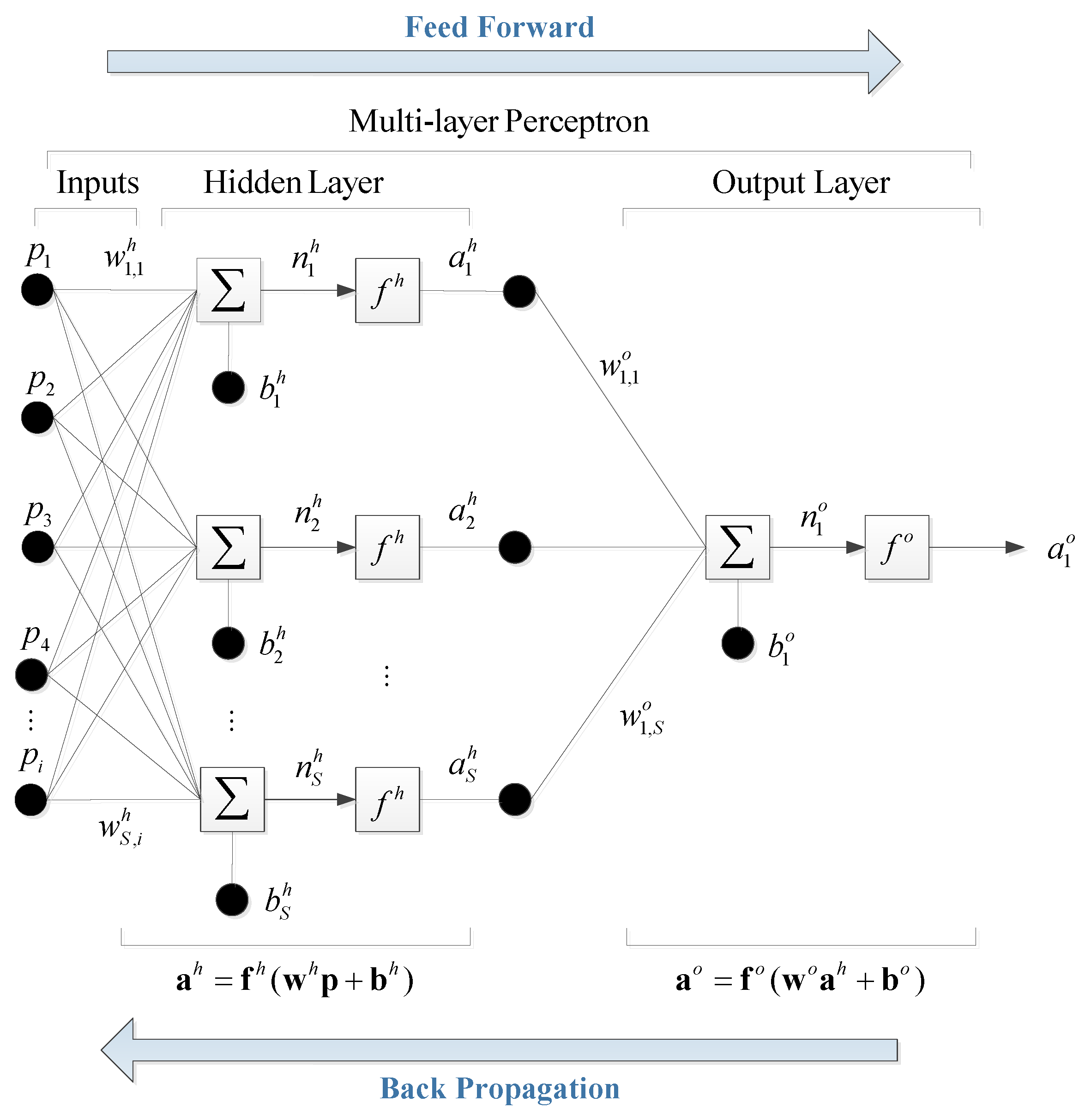
The data used for developing an ANN model is divided into two parts: the training data for training the model and the test data for verifying or testing the performance of the trained model. The training data should be sampled to represent the characteristics of the population. Otherwise, the model would not perform well for the cases that had not been encountered during the training. For example, if a variable of the training data consists of only relatively small values, the model would not perform well for large values of the variable because the model has not experienced the large values and vice versa. Therefore, in general, the size of the training data is taken to be larger than that of the test data. In the previous studies of Mase et al. [3] and Kim and Park [6], however, only 100 randomly sampled data were used for training the models, which is much smaller than the total number of data, 579 or 641. This might be one of the reasons why the ANN models do not show superior performance compared with the empirical formula (see Table 1).

To overcome this problem, the stratified sampling method is used in this study to sample 100 training data as in the previous studies while using the remaining 479 data to test the model. The key idea of stratified sampling is to divide the whole range of a variable into many sub-ranges and to sample the data so that the probability mass in each sub-range becomes similar between sample and population. Since a number of variables are involved in this study, the sampling was done manually. There are two kinds of statistical tests to evaluate the performance of stratified sampling, i.e., parametric and non-parametric tests. Since the probability mass function of each variable in this study does not follow the normal distribution, the chi-square (${\mathsf{\chi }}^2$) test is used, which is one of the non-parametric tests. The test is fundamentally based on the error between the assumed and observed probability densities [29]. In the test, each of the range of the $n$ observed data is divided into $m$ sub-ranges. In addition, the number of frequencies ($n_i$) of the variable in the $i$th sub-range is counted. Furthermore, the observed frequencies ($n_i,i=1\text{ to }m$) and the corresponding theoretical frequencies ($e_i,i=1\text{ to }m$) of an assumed distribution are compared. As the total sample points $n$ tends to $\infty$, it can be shown [30] that the quantity, ${\displaystyle {\sum }_{i=1}^m{(n_i-e_i)}^2/e_i}$, approaches the ${\mathsf{\chi }}^2$ distribution with $f=m-1-k$ degree of freedom, where $k$ is the number of parameters in the assumed distribution. $k$ is set to zero for non-normal distribution. The observed distribution is considered to follow the assumed distribution with the level of significance $\mathsf{\sigma }$ if

$${\displaystyle \sum _{i=1}^m\frac{{(n_i-e_i)}^2}{e_i}<c_{1-\mathsf{\sigma },f}},$$

(4)

where $c_{1-\mathsf{\sigma },f}$ indicates the value of the ${\mathsf{\chi }}^2$ distribution with $f$ degree of freedom at the cumulative mass of $1-\mathsf{\sigma }$. In this study, a 5% level of significance is used.

Table 2. Input and output variables.

Input Variables	Output Variable
$P,N_w,S,\cot \mathsf{\alpha },H_s,T_p,h/H_s,SS$	$N_s$

shows the input and output variables in the ANN model. The surf similarity parameter was split into $\cot \mathsf{\alpha }$, $H_s$, and $T_p$ as done by Kim and Park [6]. The peak period, $T_p$, was used instead of $T_m$ because it contains the information about spectral peak as well as mean wave period. The neural network can deal with qualitative data by assigning the values to them. The permeability coefficients of impermeable core, permeable core, and homogeneous structure are assigned to 0.1, 0.5, and 0.6, respectively, as done by Van der Meer [27]. On the other hand, the spectral shapes of narrowband, medium-band (i.e., Pierson-Moskowitz spectrum), and wideband are assigned to 1.0, 0.5, and 0, as done by Mase et al. [3]. To perform the chi-square test, the range of each variable was divided into eight to 11 sub-ranges. The details of the test can be found in the thesis of Lee [31]. Here, only the residual chart calculated based on Equation (4) is presented in

Table 3. Residual chart of chi-square tests.

Range	$N_s$	$P$	$N_w$	$S$	$\cot \mathsf{\alpha }$	$H_s$	$T_p$	$h/H_s$	$SS$
1	0.09	0.26	0.03	0.42	0.13	0.06	-	-	0.31
2	0.00	-	-	0.03	-	0.00	-	1.74	-
3	0.00	-	-	0.01	0.00	1.24	-	0.00	-
4	0.00	-	-	0.01	-	0.14	0.84	0.17	-
5	0.05	-	-	0.12	0.47	0.11	0.00	0.08	0.00
6	0.10	-	-	0.14	-	0.02	0.02	0.02	-
7	0.04	-	-	0.11	-	1.24	0.00	0.06	-
8	0.07	0.35	-	0.06	-	-	0.02	0.00	-
9	0.14	-	-	0.90	-	-	0.38	-	-
10	1.50	0.04	0.03	0.45	0.08	-	-	0.14	0.37
11	-	-	-	0.43	-	-	0.52	-	-
${\displaystyle \sum {(n_i-e_i)}^2/e_i}$	1.99	0.64	0.06	2.67	0.68	2.81	1.77	2.20	0.69
$f$	9	2	1	10	3	6	6	7	2
$c_{1-\mathsf{\sigma },f}$	16.8	5.99	3.84	18.3	7.86	12.6	12.6	14.1	5.99

. Some variables are well distributed over the whole range, whereas some varies among a few sub-ranges (e.g., $P=$ 0.1, 0.5, or 0.6). Table 3 shows that Equation (4) is satisfied for all the variables, indicating that the probability mass function of each variable of the training data is significant at a 5% level of significance. As an example, the probability mass functions of the training data and population of the damage level $S$ are compared in Figure 3, showing that they are in good agreement.

3.2. ANN Model

The multi-perceptron is considered as an attractive alternative to an empirical formula in that it imitates the nonlinear relationship between input and output variables in a more simplified way. The model aims to obtain the optimized weights of the network using a training algorithm designed to minimize the error between the output and target variables by modifying the mutually connected weights. In this study, the multi-perceptron with one hidden layer is used as shown in Figure 4, where $i$ is the number of input variables.

Firstly, for each of the input and output variables, the data are normalized so that all of the data are distributed in the range of [min, max] = [–1, 1]. This can be done by subtracting the average from the data values and rescaling the resulting values in such a way that the smallest and largest values become $-1$ and 1, respectively. Secondly, the initial weights in the hidden layer are set to have random values between $-1$ and 1, and the initial biases are all set to zero. The next step is to multiply the weight matrix by the input data, $p$, and add the bias so that

$$n_k^h={\displaystyle \sum _{j=1}^J{w}_{kj}^h{p}_j}+b_k^h,k=1\text{ to }K,$$

(5)

where $J$ and $K$ are the number of input variables and hidden neurons, respectively, and $p$, $b^h$ and $w^h$ are the input variable, bias, and weight in the hidden layer, respectively. The subscripts of the weight $w_{kj}^h$ are written in such a manner that the first subscript denotes the neuron in question and the second one indicates the input variable to which the weight refers. The $n_k^h$ calculated by Equation (5) is fed into an activation function, $f^h$, to calculate $a_k^h$. Hyperbolic tangent sigmoid function is used as the activation function so that

$$a_k^h=\frac{e^{n_k^h}-e^{-n_k^h}}{e^{n_k^h}+e^{-n_k^h}}.$$

(6)

In the output layer, the same procedure as that in the hidden layer is used except that only one neuron is used so that

$$n_1^o={\displaystyle \sum _{j=1}^K{w}_{1j}^o{a}_j^h}+b_1^o,$$

(7)

and the linear activation function is used to calculate $a_1^o$ so that

$$a_1^o=n_1^o.$$

(8)

The neural network with the randomly assigned initial weights and biases cannot accurately estimate the required output. Therefore, the weights and biases are modified by the training to minimize the difference between the model output and target (observed) values. To train the network, the error function is defined as

$$\mathsf{\epsilon }={\Vert \mathsf{\tau }-a_1^o\Vert }^2,$$

(9)

where $\Vert \Vert$ denotes a norm, and $\mathsf{\tau }$ is the target value vector to be sought. To minimize the error function, the Levenberg-Marquardt algorithm is used, which is the standard algorithm of nonlinear least-squares problems. Like other numeric minimization algorithms, the Levenberg-Marquardt algorithm is an iterative procedure. It necessitates a damping parameter $\mathsf{\mu }$, and a factor $\mathsf{\theta }$ that is greater than one. In this study, $\mathsf{\mu }=0.001$ and $\mathsf{\theta }=10$ were used. If the squared error increases, then the damping is increased by successive multiplication by $\mathsf{\theta }$ until the error decreases with a new damping parameter of $\mathsf{\mu }{\mathsf{\theta }}^k$ for some $k$. If the error decreases, the damping parameter is divided by $\mathsf{\theta }$ in the next step. The training was stopped when the epoch reached 5000 or the damping parameter was too large for more training to be performed.

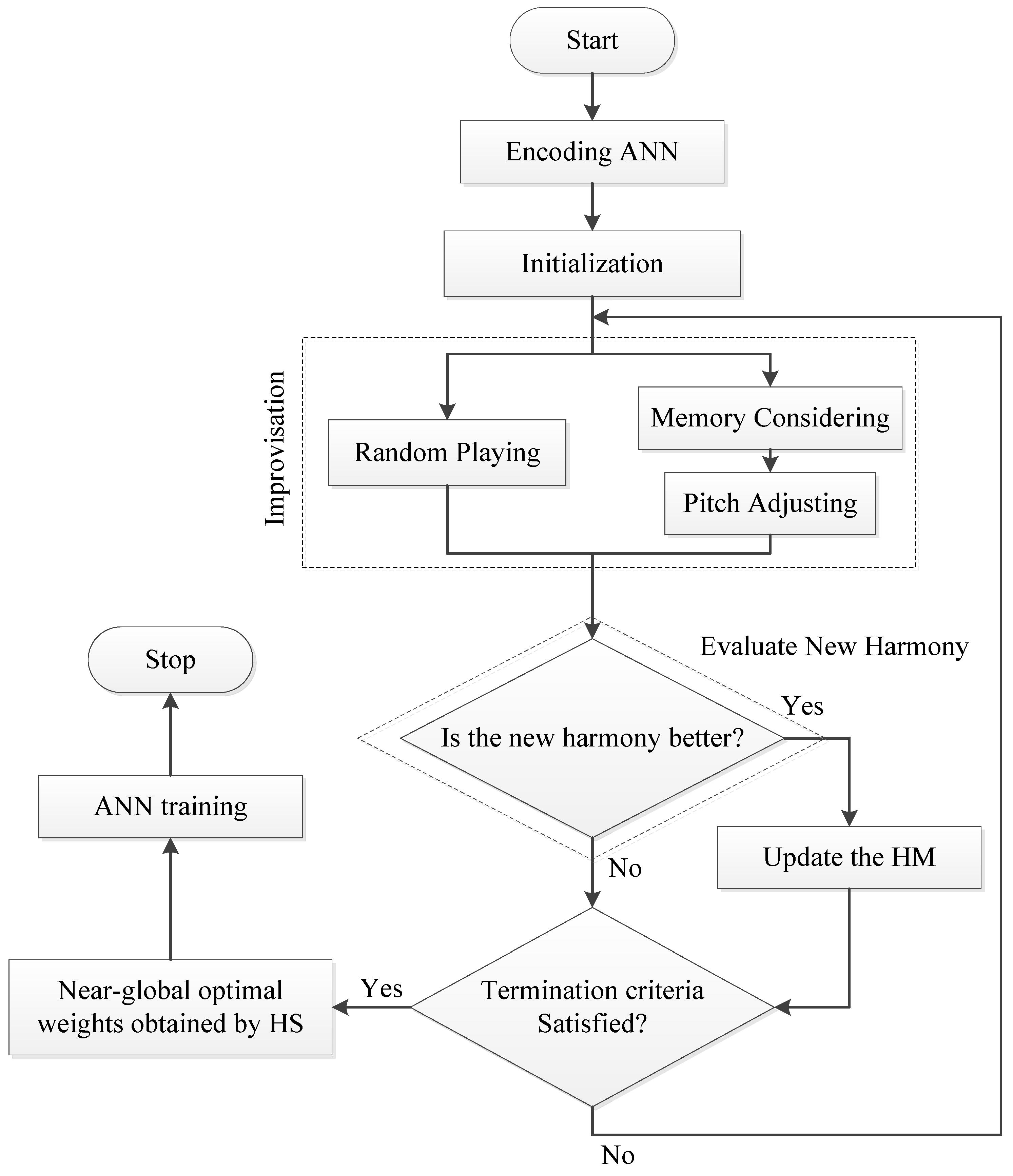
3.3. HS-ANN Hybrid Model

To find the initial weights of the ANN model that lead into the global minimum of the error function, in general, a Monte Carlo simulation is performed, that is, the training is repeated many times with different initial weights. The Monte Carlo simulation, however, takes a great computational time. In this section, we develop an HS-ANN model in which the near-global optimal initial weights are found by the HS algorithm.

The HS algorithm consists of five steps as follows [32].

Step 1. Initialization of the algorithm parameters

Generally, the problem of global optimization can be written as

$$\begin{array}{l}\text{Minimize\hspace{1em}}f(x)\\ \text{subject to\hspace{1em}}{x}_i\in X_i,i=1,2,\mathrm{...},N,\end{array}$$

(10)

where $f(x)$ is an objective function, $x$ is the set of decision variables, and $X_i$ is the set of possible ranges of the values of each decision variable, which can be denoted as $X_i=\left\{x_i(1),x_i(2),\mathrm{...},x_i(K)\right\}$ for discrete decision variables satisfying $x_i(1)<x_i(2)<\cdots <x_i(K)$ or ${}_{L}x_i\le X_i\le {}_{U}x_i$ for continuous decision variables. In addition, $N$ is the number of decision variables and $K$ is the number of possible values for the discrete variables. In addition, HS algorithm parameters exist that are required to solve the optimization problems: harmony memory size (HMS, number of solution vectors), harmony memory considering rate (HMCR), pitch adjusting rate (PAR) and termination criterion (maximum number of improvisation). HMCR and PAR are the parameters used to improve the solution vector.

Step 2. Initialization of harmony memory

The harmony memory (HM) matrix is composed of as many randomly generated solution vectors as the size of the HM, as shown in Equation (11). They are stored with the values of the objective function, $f(x)$, ascendingly:

$$\text{HM}=\left[\begin{array}{c}{x}^1\\ x^2\\ ⋮\\ x^{\text{HMS}}\end{array}\right].$$

(11)

Step 3. Improvise a new harmony from the HM

A new harmony vector, $x^{\prime }=\left(x_1^{\prime },x_2^{\prime },\mathrm{...},x_N^{\prime }\right)$, is created from the HM based on assigned HMCR, PAR, and randomization. For example, the value of the first decision variable $\left(x_1^{\prime }\right)$ for the new vector can be selected from any value in the designated HM range, $x_1^1~x_1^{\text{HMS}}$. In the same way, the values of other decision variables can be selected. The HMCR parameter, which varies between 0 and 1, is a possibility that the new value is selected from the HM as follows:

$$x_i^{\prime }\leftarrow \{\begin{array}{ll}{x}_i^{\prime }\in \left\{x_i^1,x_i^2,\mathrm{...},x_i^{\text{HMS}}\right\}& \text{ with probability of HMCR}\\ x_i^{\prime }\in X_i& \text{ with probability of }(1-\text{HMCR}),\end{array}$$

(12)

The HMCR is the probability of selecting one value from the historic values stored in the HM, and the value (1-HMCR) is the probability of randomly taking one value from the possible range of values. This procedure is analogous to the mutation operator in genetic algorithms. For instance, if a HMCR is 0.95, the HS algorithm would pick the decision variable value from the HM including historically stored values with a 95% of probability. Otherwise, with a 5% of probability, it takes the value from the entire possible range. A low memory considering rate selects only a few of the best harmonies, and it may converge too slowly. If this rate is near 1, most of the pitches in the harmony memory are used, and other ones are not exploited well, which does not lead to good solutions. Therefore, typically $\text{HMCR}=0.7-0.95$ is recommended.

On the other hand, the HS algorithm would examine every component of the new harmony vector, $x^{\prime }=\left(x_1^{\prime },x_2^{\prime },\mathrm{...},x_N^{\prime }\right)$, to decide whether it has to be pitch-adjusted or not. In this procedure, the PAR parameter which sets the probability of adjustment for the pitch from the HM is used as follows:

$$\text{Pitch adjusting decision for }{x}_i^{\prime }\leftarrow \{\begin{array}{ll}\text{Yes}& \text{ with probability of PAR}\\ \text{No}& \text{ with probability of }(1-\text{PAR}).\end{array}$$

(13)

The pitch adjusting procedure is conducted only after a value is selected from the HM. The value (1−PAR) is the probability of doing nothing. To be specific, if the value of PAR is 0.1, the algorithm will take a neighboring value with $0.1\times \text{HMCR}$ probability. For example, if the decision for $x_i^{\prime }$ in the pitch adjustment process is Yes, and $x_i^{\prime }$ is considered to be $x_i(k)$, then the kth element in $X_i$, or the pitch-adjusted value of $x_i(k)$, is changed into

$$\begin{array}{ll}{x}_i^{\prime }\leftarrow x_i(k+m)& \text{ for discrete decision variables}\\ x_i^{\prime }\leftarrow x_i^{\prime }+\mathsf{\alpha }& \text{ for continuous decision variables},\end{array}$$

(14)

where m is the neighboring index, $m\in \left\{\mathrm{...},-2,-1,1,2,\mathrm{...}\right\}$, $\mathsf{\alpha }$ is the value of $bw\times u(-1,1)$, $bw$ is an arbitrarily chosen distance bandwidth or fret width for the continuous variable, and $u(-1,1)$ is a random number from uniform distribution with the range of $[-1,1]$. If the pitch-adjusting rate is very low, because of the limitation in the exploration of a small subspace of the whole search space, it slows down the convergence of HS. On the contrary, if the rate is very high, it may cause the solution to scatter around some potential optima. Therefore, $\text{PAR}=0.1-0.5$ is used in most applications. The parameters HMCR and PAR help the HS algorithm to search globally and locally, respectively, to improve the solution.

Step 4. Evaluate new harmony and update the HM

This step is to evaluate the new harmony and update the HM if necessary. Evaluating a new harmony means that the new harmony (or solution vector) is used in the objective function and the resulting functional value is compared with the solution vector in the existing HM. If the new harmony vector gives better performance than the worst harmony in the HM, evaluated in terms of the value of objective function, the new harmony would be included in the harmony memory and the existing worst harmony is eliminated from the harmony memory. In this study, the mean square error function is used as the objective function for both HS optimization and ANN training.

Step 5. Repeat Steps 3 and 4 until the termination criterion is satisfied

The iterations are terminated if the stop criterion is satisfied. If not, Steps 3 and 4 would be repeated. The pseudo-code of the HS algorithm is given in Figure 5. The initial weights optimized by the HS algorithm are then further trained by a gradient descent algorithm. This method is denoted as an HS-ANN model, and it can be expressed as the flow chart in Figure 6.

4. Result and Discussion

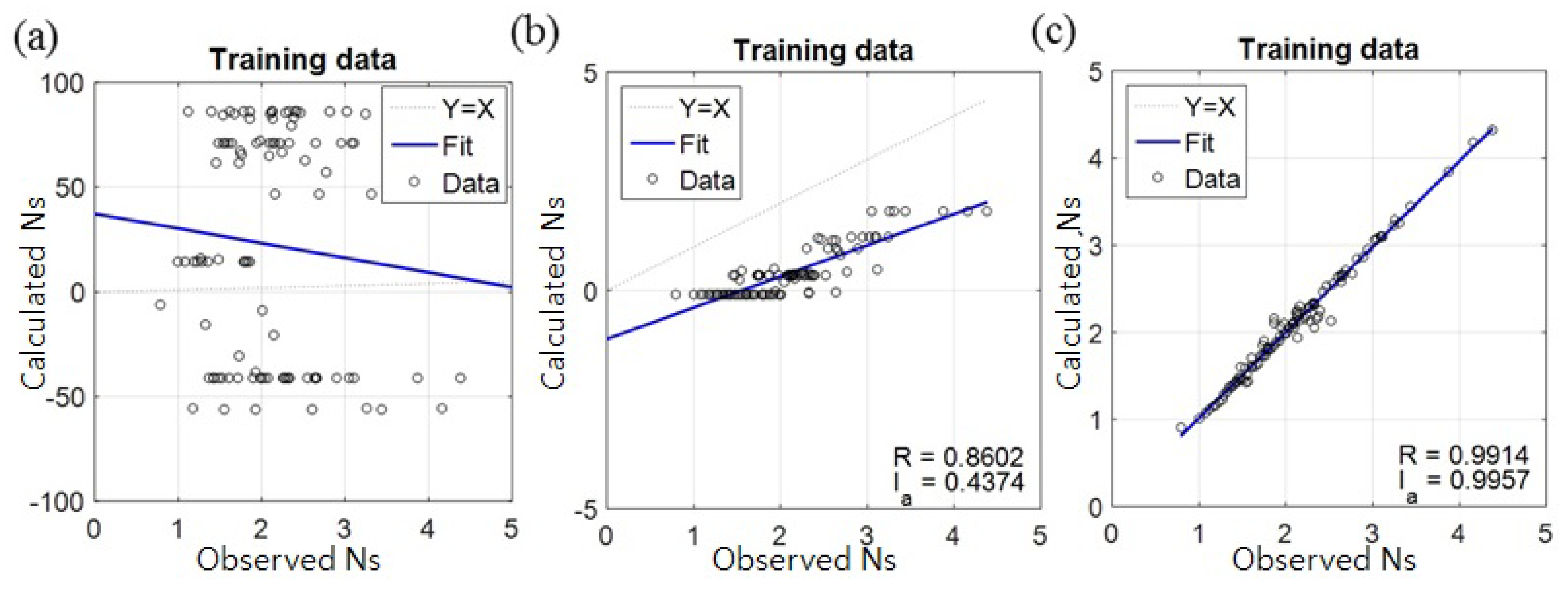
4.1. Assessment of Accuracy and Stability of the Models

In this section, the accuracy and stability are compared between the conventional ANN model without using the HS algorithm and the HS-ANN hybrid model. Both models were run 50 times, and the statistical analyses were conducted for the model results. Each of the HMCR and PAR of the HS algorithm were chosen to vary from 0.1 to 0.9 at intervals of 0.2, so a total of 25 HS-ANN models were tested. The models were used to estimate the stability number of rock armor for the experimental data of Van der Meer [26] for which the input and output variables are given as in Table 2. The 579 experimental data excluding the data of low-crested structures were used, as done by Mase et al. [3]. As described in Section 3.1, a hundred data sampled by the stratified sampling method were used to train the ANN, whereas the remaining 479 data were used to test the model.

The correlation coefficient ($r$) and index of agreement ($I_a$) between model output values and target values of the 479 test data are used to evaluate the performance of the models. First, to compare the accuracy of the developed models with those of previous studies (see Table 1), the maximum value of correlation coefficient among 50 runs of each model is presented in

Table 4. Maximum values of correlation coefficient.

HS-ANN	HMCR\PAR	0.1	0.3	0.5	0.7	0.9
	0.1	0.957	0.971	0.961	0.9731	0.964
	0.3	0.959	0.967	0.970	0.9723	0.960
	0.5	0.961	0.954	0.961	0.957	0.968
	0.7	0.968	0.9732	0.959	0.967	0.970
	0.9	0.9715	0.970	0.9724	0.970	0.960
ANN	0.971

. For the results of the HS-ANN models, the rank is indicated by a superscript, and the largest two values are shaded. The largest correlation coefficient of the HS-ANN model is only slightly larger than that of the ANN model, but both of them are much greater than those of previous studies (see Table 1), probably because the stratified sampling was used in the present study.

Even though we used the correlation coefficient to compare the accuracy of our model results with those of previous studies, it is not a good indicator for model accuracy because it merely evaluates the linearity between observation and prediction but not the agreement between them. Hereinafter, we use the index of agreement introduced by Willmott [34] as a measure of the degree to which a model’s predictions are error-free but not a measure of correlation between the observed and predicted variates. The index of agreement is given as

$$I_a=1-\frac{{\displaystyle {\sum }_{i=1}^N{\left(p_i-o_i\right)}^2}}{{\displaystyle {\sum }_{i=1}^N{\left[|p_i-\overline{o}|+|o_i-\overline{o}|\right]}^2}},$$

(15)

where $p_i$ and $o_i$ denote the predicted and observed variates, and $\overline{o}$ is the mean of the observed variates. The values for $I_a$ vary between 0 and 1.0, where 1.0 indicates perfect agreement between observations and predictions, and 0 connotes complete disagreement.

The statistical parameters used to measure the predictive ability and stability of the models are the average, standard deviation, and the minimum value of $I_a$. The larger the average, the better the overall predictive ability of the model. The smaller the standard deviation, the higher the stability of the model, that is, the less variability among the model outputs from different runs of the model. Lastly, the larger the minimum value of $I_a$, the larger the lower threshold of the predictive ability of the model. In summary, a large average and large minimum value of $I_a$ signify that the predictive ability of the model is excellent. On the other hand, a small standard deviation signifies that the model is stable.

The statistical parameters for the index of agreement are presented in

Table 5. Statistical parameters for index of agreement.

Average
HS-ANN	HMCR\PAR	0.1	0.3	0.5	0.7	0.9
	0.1	0.885	0.926	0.872	0.843	0.905
	0.3	0.934	0.910	0.913	0.914	0.912
	0.5	0.913	0.929	0.929	0.934	0.929
	0.7	0.881	0.929	0.9481	0.9443	0.9404
	0.9	0.9482	0.935	0.913	0.9375	0.892
ANN	0.804
Standard Deviation
HS-ANN	HMCR\PAR	0.1	0.3	0.5	0.7	0.9
	0.1	0.205	0.120	0.245	0.277	0.158
	0.3	0.137	0.175	0.155	0.183	0.189
	0.5	0.178	0.101	0.104	0.073	0.138
	0.7	0.224	0.130	0.0211	0.0313	0.0425
	0.9	0.0232	0.110	0.168	0.0314	0.200
ANN	0.317
Minimum Value
HS-ANN	HMCR\PAR	0.1	0.3	0.5	0.7	0.9
	0.1	0.001	0.216	0.001	0.001	0.002
	0.3	0.002	0.001	0.029	0.004	0.002
	0.5	0.003	0.319	0.254	0.468	0.003
	0.7	0.001	0.051	0.8891	0.8523	0.7105
	0.9	0.8852	0.196	0.013	0.8014	0.005
ANN	0.001
Maximum Value
HS-ANN	HMCR\PAR	0.1	0.3	0.5	0.7	0.9
	0.1	0.978	0.985	0.980	0.9871	0.981
	0.3	0.979	0.983	0.985	0.986	0.979
	0.5	0.980	0.977	0.980	0.978	0.984
	0.7	0.984	0.9862	0.979	0.983	0.985
	0.9	0.985	0.985	0.986	0.985	0.980
ANN	0.985

. Again, for the results of the HS-ANN models, the rank is indicated by a superscript, and the largest (or smallest) two values are shaded. Even though the maximum values of $I_a$ are also given, they are not discussed further because their variation is not so large to explain the difference of predictive ability or stability depending on the models. It is shown that the HS-ANN model gives the most excellent predictive ability and stability with HMCR = 0.7 and PAR = 0.5 or HMCR = 0.9 and PAR = 0.1. This result corresponds to Geem [33] who suggested that the optimal ranges of HMCR = 0.7–0.95 and PAR = 0.1–0.5. Comparing the statistical parameters between the best HS-ANN model and the ANN model, the HS-ANN model with proper values of HMCR and PAR can give much better and stable prediction than the conventional ANN model. In particular, the small value of standard deviation of the HS-ANN model indicates that the model is excellent in finding the global minimum of the error function.

4.2. Aspect of Transition of Weights

There are two major components in metaheuristic algorithms: diversification and intensification [33]. These two components seem to be contradicting each other, but balancing their combination is crucial and important to the success of a metaheuristic algorithm. In the HS algorithm, diversification is controlled by the pitch adjustment and randomization, whereas intensification is represented by the harmony memory considering rate. Therefore, in this section, the results of training of neural networks for two different cases are compared and examined, i.e., the best combination and worst combination of HMCR and PAR. The case of the HS optimization with HMCR of 0.7 and PAR of 0.5 is chosen to be the best case (Case 1) since it has the largest average and smallest standard deviation of $I_a$. The worst case (Case 2) is the case of HMCR of 0.1 and PAR of 0.5, which has the smallest average and largest standard deviation of $I_a$. The optimization process of the HS algorithm regarding the weights of neural network is illustrated in Figure 7 and Figure 8 for each case of parameter combination. Note that the results shown in these figures are those from one of the fifty runs described in the previous section. In the figures, each scatter plot indicates the relationship between calculated and observed stability numbers using (a) randomly selected initial weights; (b) optimal initial weights determined by HS algorithm; and (c) further trained weights after BP algorithm. The correlation coefficients and indices of agreement are also given.

The first graphs in Figure 7 and Figure 8 show that the stability numbers calculated by using the randomly selected initial weights are distributed in a wide range from large negative values to large positive values and have very weak and negative correlation with the observed stability numbers. The second graphs show that the stability numbers calculated by using the optimal initial weights determined by the HS algorithm are distributed within the range of 0 to 5 as they are in the observation. Case 1 shows much better correlation between calculation and observation than the Case 2, whereas the index of agreement of Case 1 is only slightly better than that of Case 2. The calculated stability numbers in Case 1 show strong correlation with the observed ones, but they are underestimated as a whole. The third graphs after further training by the BP algorithm show very strong correlation and good agreement between calculation and observation. Even Case 2 (the worst case) shows quite high value of index of agreement compared with the values for HMCR = 0.1 and PAR = 0.5 in Table 5. Note that the results in Figure 7 and Figure 8 are for training data, whereas those in Table 5 are for test data.

4.3. Computational Time

Most of the computational time of the conventional ANN model is used for the BP training of the model, whereas the HS-ANN model needs computational time for finding the optimal initial weights using the HS algorithm and then for finding the global minimum of the error function by the BP training. Lee [31] compared the computational time between the conventional ANN model and the HS-ANN models with various combinations of HMCR and PAR. Since the statistical characteristics of computational time do not show a big difference among different combinations of HMCR and PAR, here we only present the case of HMCR = 0.7 and PAR = 0.5 for which the HS-ANN model gives the most excellent predictive ability and stability.

Table 6. Statistical characteristics of computational time (unit = s).

Algorithm	HS-ANN Model		Conventional ANN Model
	Average	SD	Average	SD
HS	285.6	7.8	-	-
BP	102.9	55.2	68.6	95.0
Total	385.5	55.7	68.6	95.0

shows the average and standard deviation (SD) of the computational times of the 50 runs of each model. The total computational time of the HS-ANN model is five to six times greater than that of the conventional ANN model. In spite of the greater computing time, it is worthwhile to use the HS-ANN model because it gives much more accurate and stable prediction than the conventional ANN model with a small number of simulations. It is interesting to note that the computing time for the BP training of the HS-ANN model is greater than that of the conventional ANN model probably because it takes a longer time to reach the global minimum which is smaller than the local minimums as shown in Figure 1. On the other hand, the standard deviation of the BP training of the HS-ANN model is smaller than that of the conventional ANN model because the HS-ANN model starts the BP training from the optimal initial weights whose variation is not so large. The standard deviation of the HS algorithm is very small because the maximum number of improvisation was set to 100,000.

5. Conclusion

In this study, an HS-ANN hybrid model was developed to predict the stability number of breakwater armor stones based on the experimental data of Van der Meer [26]. The HS algorithm was used to find the near-global optimal initial weights, which were then used in the BP training to find the true global minimum of the error function by the Levenberg-Marquardt algorithm. The stratified sampling was used to sample the training data. A total of 25 HS-ANN models were tested with five different values for both HMCR and PAR varying from 0.1 to 0.9 at intervals of 0.2. The HS-ANN models were compared with the conventional ANN model which uses a Monte Carlo simulation to determine the initial weights. The correlation coefficient and index of agreement were calculated to evaluate the performance of the models. Each model was run 50 times and the statistical analyses were conducted for the model results. The major findings are as follows:

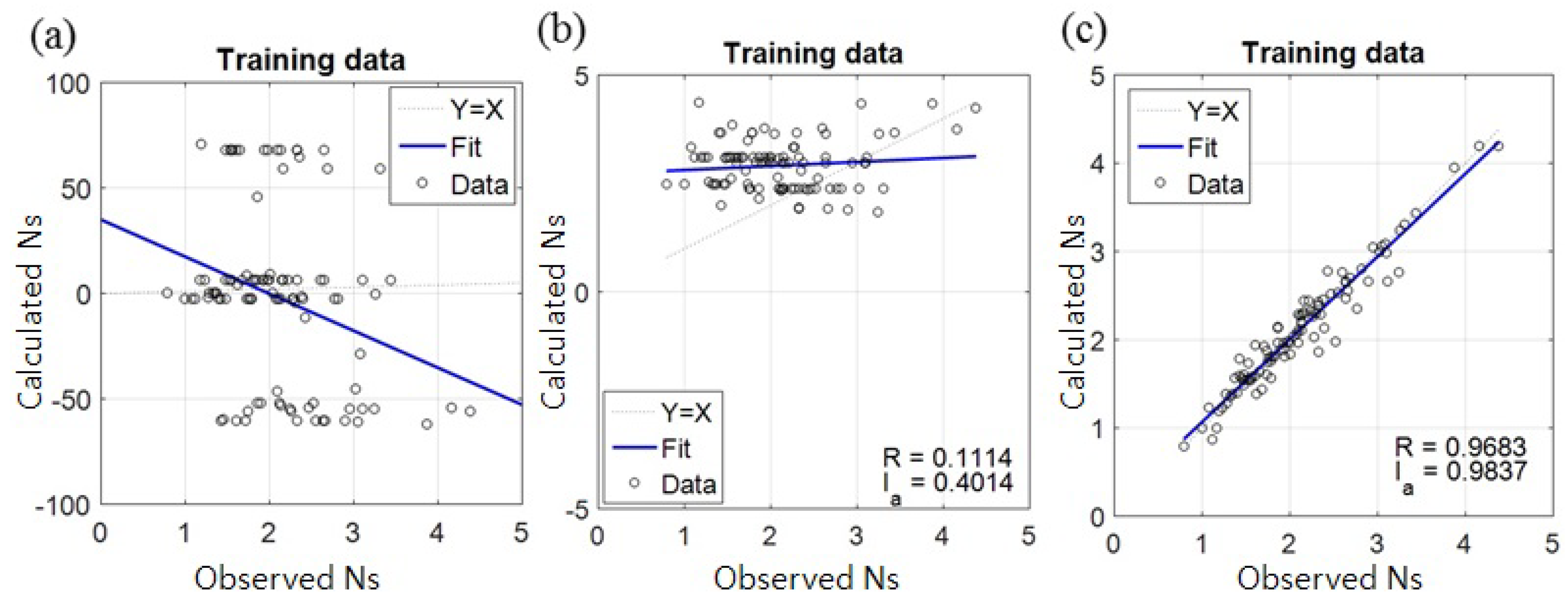
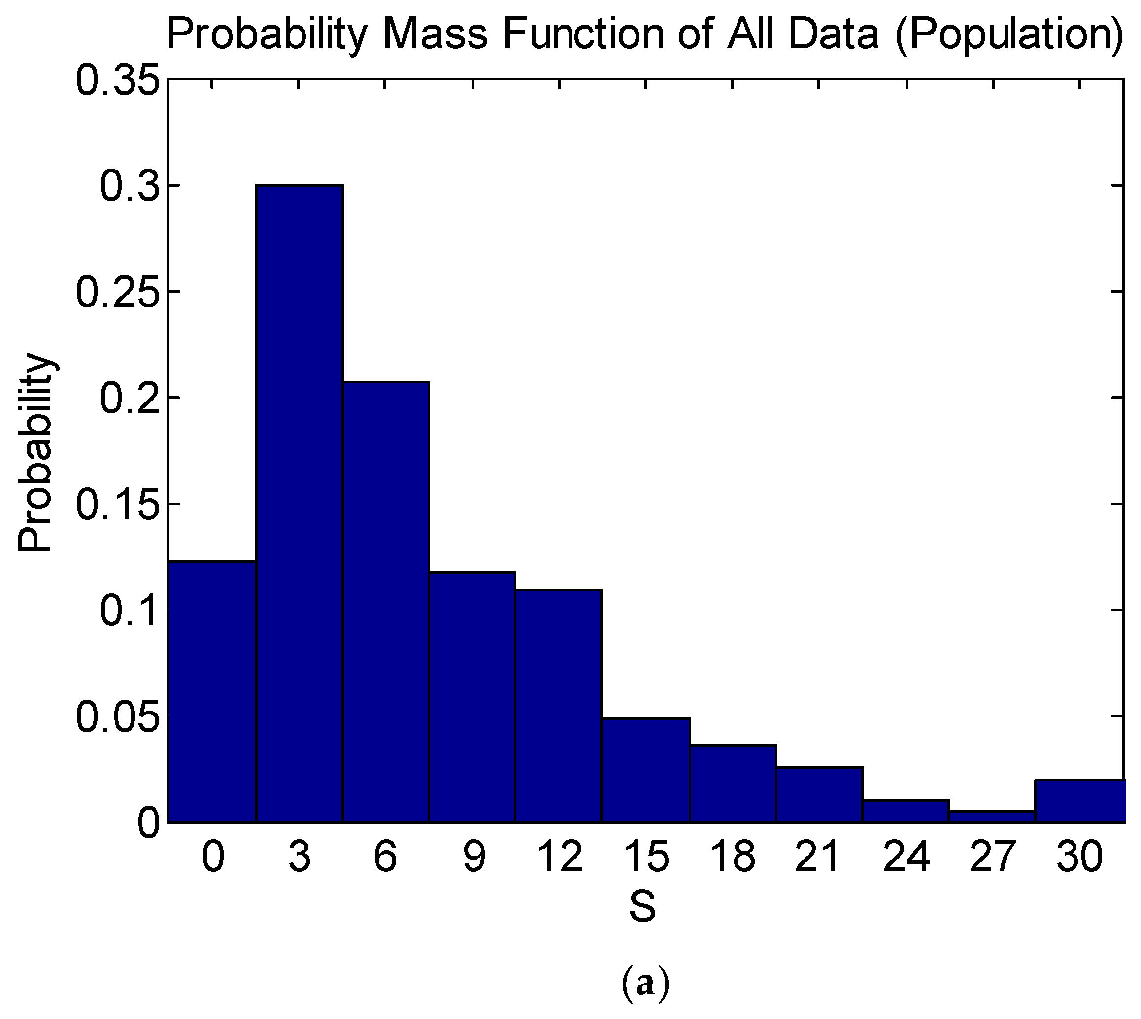
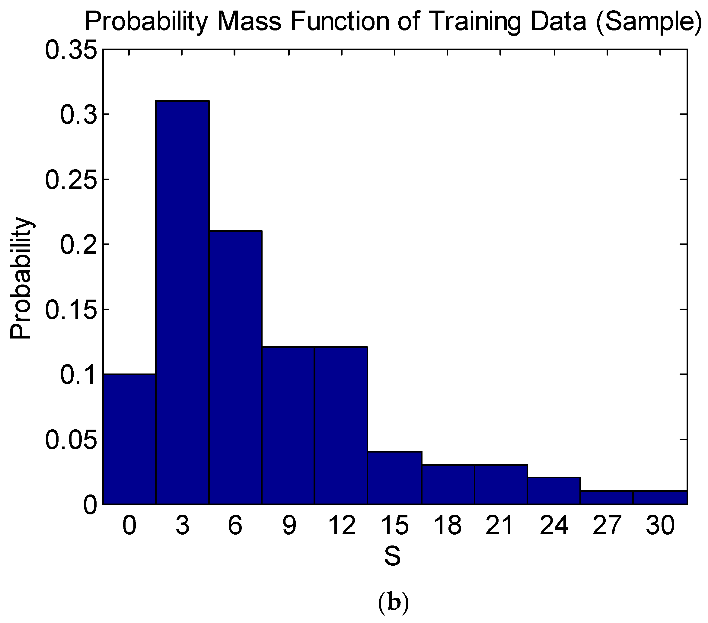
• The correlation coefficients of the present study were greater than those of previous studies probably because of the use of stratified sampling.
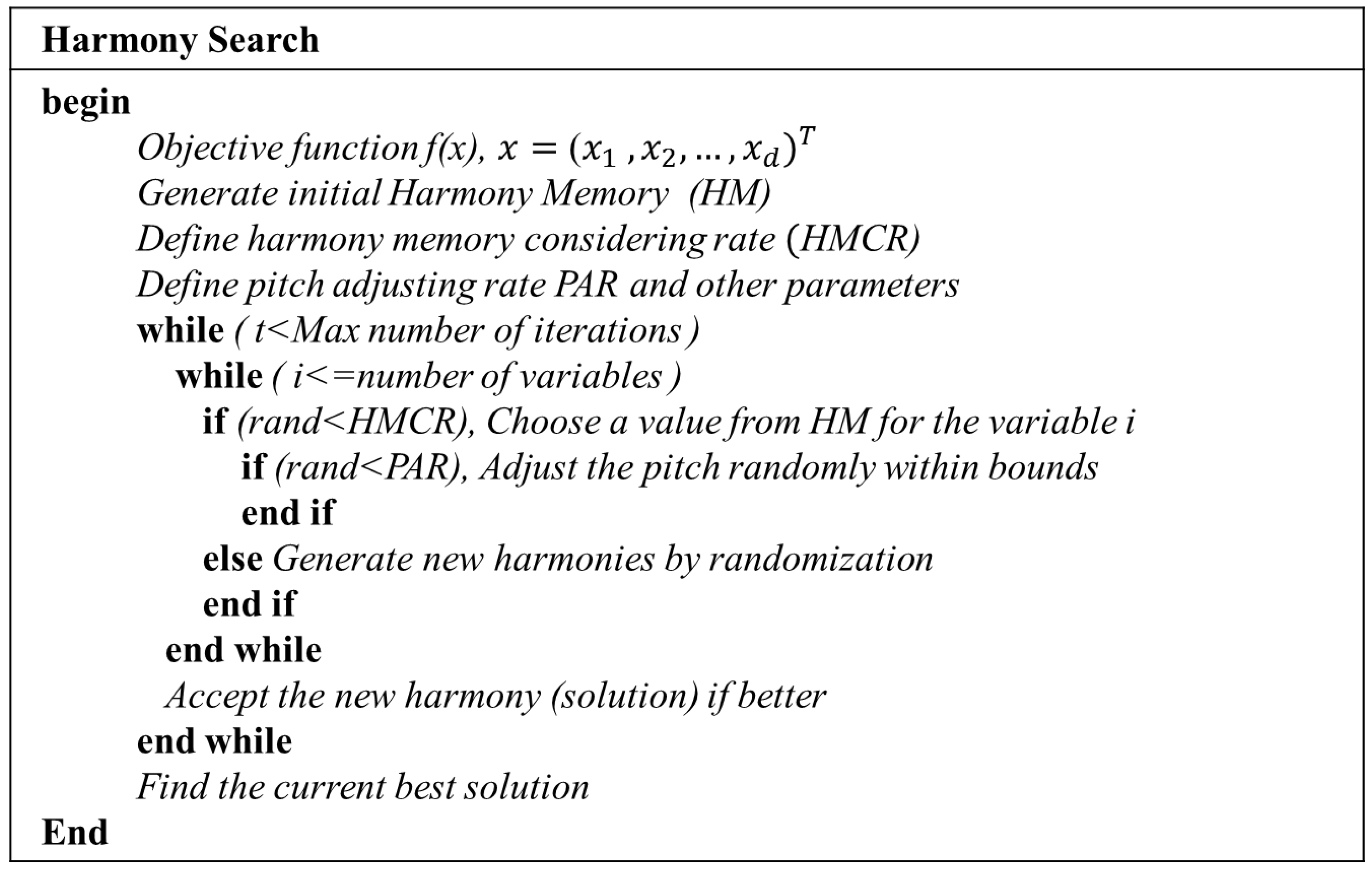
• In terms of the index of agreement, the HS-ANN model gave the most excellent predictive ability and stability with HMCR = 0.7 and PAR = 0.5 or HMCR = 0.9 and PAR = 0.1, which correspond to Geem [33] who suggested the optimal ranges of HMCR = 0.7–0.95 and PAR = 0.1–0.5 for the HS algorithm.
• The statistical analyses showed that the HS-ANN model with proper values of HMCR and PAR can give much better and more stable prediction than the conventional ANN model.
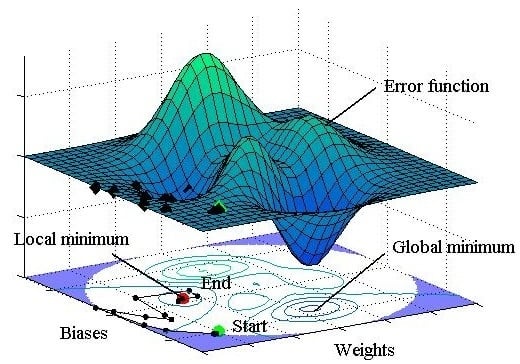
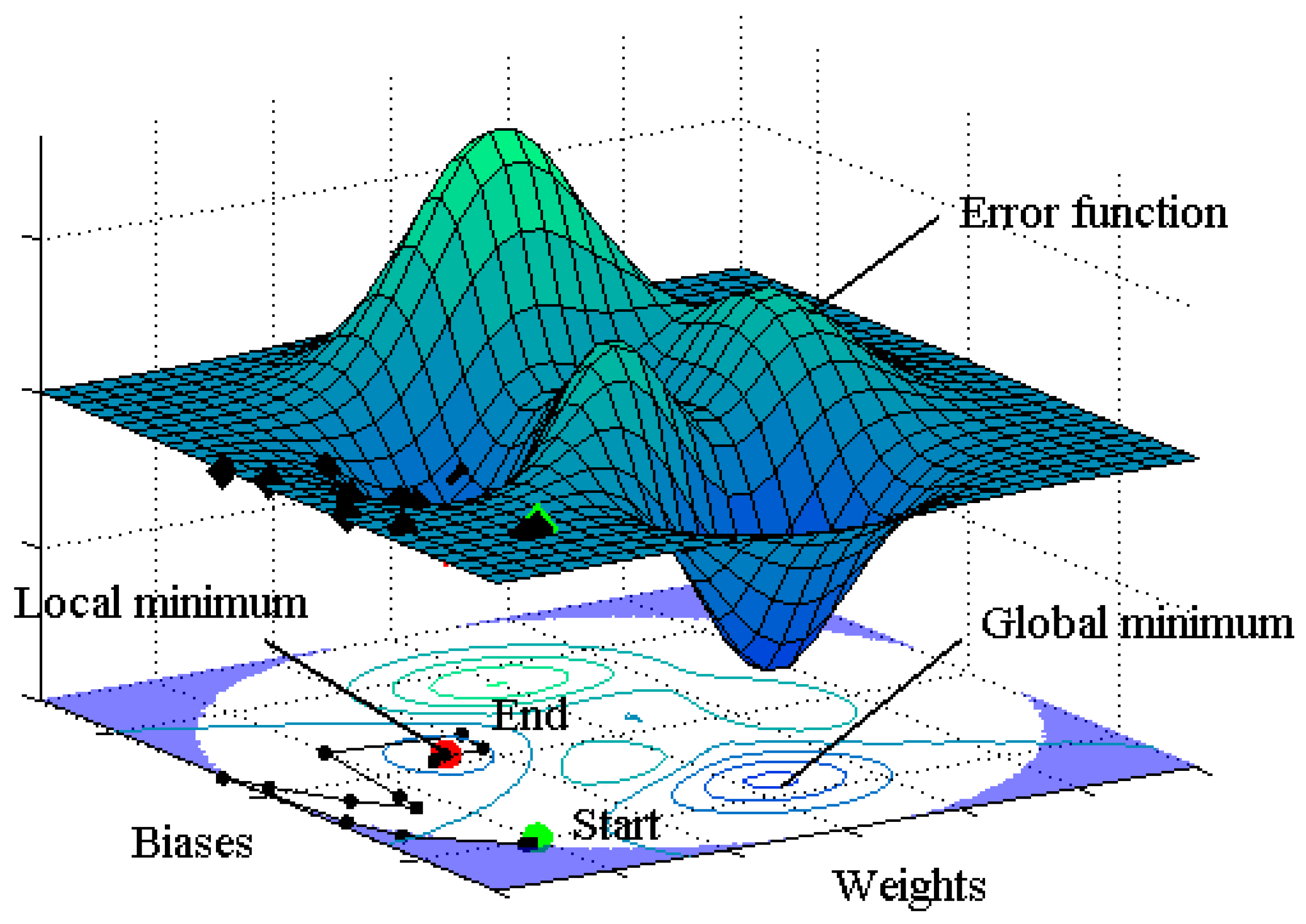
• The HS algorithm was found to be excellent in finding the global minimum of an error function. Therefore, the HS-ANN hybrid model would solve the local minimization problem of the conventional ANN model using a Monte Carlo simulation, and thus could be used as a robust and reliable ANN model not only in coastal engineering but also other research areas.

In the future, the present HS-ANN model could be compared with other hybrid ANN models using different heuristic algorithms such as genetic algorithm (GA), particle swarm optimization (PSO), and Cuckoo Search (CS). Not only GA [18,35,36] but also PSO [37,38] and CS [39] have been applied for neural network training. Analyzing and comparing those hybrid ANN models would provide a way to find the most suitable heuristic algorithm for determining the optimal initial weights for ANN.

References

1. McCulloch, W.S.; Pitts, W. A logical calculus of the ideas immanent in nervous activity. Bull. Math. Biol. 1990, 52, 99–115. [Google Scholar] [CrossRef]
2. Rumelhart, D.E.; Hinton, G.E.; Williams, R.J. Learning representations by back-propagating errors. Nature 1986, 323, 533–536. [Google Scholar] [CrossRef]
3. Mase, H.; Sakamoto, M.; Sakai, T. Neural network for stability analysis of rubble-mound breakwaters. J. Waterway Port Coast. Ocean Eng. 1995, 121, 294–299. [Google Scholar] [CrossRef]
4. Tsai, C.P.; Lee, T. Back-propagation neural network in tidal-level forecasting. J. Waterway Port Coast. Ocean Eng. 1999, 125, 195–202. [Google Scholar] [CrossRef]
5. Cox, D.T.; Tissot, P.; Michaud, P. Water level observations and short-term predictions including meteorological events for entrance of Galveston Bay, Texas. J. Waterway Port Coast. Ocean Eng. 2002, 128, 1–29. [Google Scholar] [CrossRef]
6. Kim, D.H.; Park, W.S. Neural network for design and reliability analysis of rubble mound breakwaters. Ocean Eng. 2005, 32, 1332–1349. [Google Scholar] [CrossRef]
7. Van Gent, M.R.A.; Van den Boogaard, H.F.P.; Pozueta, B.; Medina, J.R. Neural network modeling of wave overtopping at coastal structures. Coast. Eng. 2007, 54, 586–593. [Google Scholar] [CrossRef]
8. Browne, M.; Castelle, B.; Strauss, D.; Tomlinson, R.; Blumenstein, M.; Lane, C. Near-shore swell estimation from a global wind–wave model: Spectral process, linear and artificial neural network models. Coast. Eng. 2007, 54, 445–460. [Google Scholar] [CrossRef]
9. Balas, C.E.; Koc, M.L.; Tür, R. Artificial neural networks based on principal component analysis, fuzzy systems and fuzzy neural networks for preliminary design of rubble mound breakwaters. Appl. Ocean Res. 2010, 32, 425–433. [Google Scholar] [CrossRef]
10. Yoon, H.D.; Cox, D.T.; Kim, M.K. Prediction of time-dependent sediment suspension in the surf zone using artificial neural network. Coast. Eng. 2013, 71, 78–86. [Google Scholar] [CrossRef]
11. Rabunal, J.R.; Dorado, J. Artificial Neural Networks in Real-Life Applications; Idea Group Publishing: Hershey, PA, USA, 2006. [Google Scholar]
12. Haykin, S. Neural Networks: A Comprehensive Foundation; Prentice Hall: Upper Saddle River, NJ, USA, 1999. [Google Scholar]
13. Rocha, M.; Cortez, P.; Neves, J. Evolutionary neural network learning. In Progress in Artificial Intelligence; Pires, F.M., Abreu, S., Eds.; Springer Berlin Heidelberg: Heidelberg, Germany, 2003; Volume 2902, pp. 24–28. [Google Scholar]
14. Krenker, A.; Bester, J.; Kos, A. Introduction to the artificial neural networks. In Artificial Neural Networks—Methodological Advances and Biomedical Applications; Suzuki, K., Ed.; InTech: Rijeka, Croatia, 2011; pp. 15–30. [Google Scholar]
15. Kolen, J.F.; Pollack, J.B. Back Propagation Is Sensitive to Initial Conditions. In Proceedings of the Advances in Neural Information Processing Systems 3, Denver, CO, USA, 26–29 November 1990; Lippmann, R.P., Moody, J.E., Touretzky, D.S., Eds.; Morgan Kaufmann: San Francisco, CA, USA, 1990; pp. 860–867. [Google Scholar]
16. Yam, Y.F.; Chow, T.W.S. Determining initial weights of feedforward neural networks based on least-squares method. Neural Process. Lett. 1995, 2, 13–17. [Google Scholar] [CrossRef]
17. Venkatesan, D.; Kannan, K.; Saravanan, R. A genetic algorithm-based artificial neural network model for the optimization of machining processes. Neural Comput. Appl. 2009, 18, 135–140. [Google Scholar] [CrossRef]
18. Chang, Y.-T.; Lin, J.; Shieh, J.-S.; Abbod, M.F. Optimization the initial weights of artificial neural networks via genetic algorithm applied to hip bone fracture prediction. Adv. Fuzzy Syst. 2012, 2012, 951247. [Google Scholar] [CrossRef]
19. Mulia, I.E.; Tay, H.; Roopsekhar, K.; Tkalich, P. Hybrid ANN-GA model for predicting turbidity and chlorophyll-a concentration. J. Hydroenv. Res. 2013, 7, 279–299. [Google Scholar] [CrossRef]
20. Krogh, A.; Vedelsby, J. Neural network ensembles, cross validation and active learning. Adv. Neural Inf. Process. Syst. 1995, 7, 231–238. [Google Scholar]
21. Boucher, M.A.; Perreault, L.; Anctil, F. Tools for the assessment of hydrological ensemble forecasts obtained by neural networks. J. Hydroinf. 2009, 11, 297–307. [Google Scholar] [CrossRef]
22. Zamani, A.; Azimian, A.; Heemink, A.; Solomatine, D. Wave height prediction at the Caspian Sea using a data-driven model and ensemble-based data assimilation methods. J. Hydroinf. 2009, 11, 154–164. [Google Scholar] [CrossRef]
23. Kim, S.E. Improving the Generalization Accuracy of ANN Modeling Using Factor Analysis and Cluster Analysis: Its Application to Streamflow and Water Quality Predictions. Ph.D. Thesis, Seoul National University, Seoul, Korea, 2014. [Google Scholar]
24. Geem, Z.W.; Kim, J.H.; Loganathan, G.V. A new heuristic optimization algorithm: Harmony search. Simulation 2001, 76, 60–68. [Google Scholar] [CrossRef]
25. Hudson, R.Y. Laboratory investigation of rubble-mound breakwaters. J. Waterways Harbors Div. 1959, 85, 93–121. [Google Scholar]
26. Van der Meer, J.W. Rock Slopes and Gravel Beaches under Wave Attack; Delft Hydraulics Communication No. 396: Delft, The Netherlands, 1988. [Google Scholar]
27. Van der Meer, J.W. Stability of breakwater armor layers—Design formulae. Coast. Eng. 1987, 11, 93–121. [Google Scholar] [CrossRef]
28. Smith, W.G.; Kobayashi, N.; Kaku, S. Profile Changes of Rock Slopes by Irregular Waves. In Proceedings of the 23rd International Conference on Coastal Engineering, Venice, Italy, 4–9 October 1992; Edge, B.L., Ed.; American Society of Civil Engineers: Reston, VA, USA, 1992; pp. 1559–1572. [Google Scholar]
29. Haldar, A.; Mahadevan, S. Reliability Assessment Using Stochastic Finite Element Analysis; John Wiley & Sons: New York, NY, USA, 2000. [Google Scholar]
30. Hoel, P.G. Introduction to Mathematical Statistics, 3rd ed.; Wiley & Sons: New York, NY, USA, 1962. [Google Scholar]
31. Lee, A. Determination of Near-Global Optimal Initial Weights of Artificial Neural Networks Using Harmony Search Algorithm: Application to Breakwater Armor Stones. Master’s Thesis, Seoul National University, Seoul, Korea, 2016. [Google Scholar]
32. Lee, K.S.; Geem, Z.W. A new structural optimization method based on the harmony search algorithm. Comput. Struct. 2004, 82, 781–798. [Google Scholar] [CrossRef]
33. Geem, Z.W. Music-Inspired Harmony Search Algorithm; Springer: Berlin, Germany, 2009. [Google Scholar]
34. Willmott, C.J. On the validation of models. Phys. Geol. 1981, 2, 184–194. [Google Scholar]
35. Whitley, D.; Starkweather, T.; Bogart, C. Genetic algorithms and neural networks: Optimizing connections and connectivity. Parallel Comput. 1990, 14, 347–361. [Google Scholar] [CrossRef]
36. Hozjan, T.; Turk, G.; Fister, I. Hybrid artificial neural network for fire analysis of steel frames. In Adaptation and Hybridization in Computational Intelligence; Fister, I., Ed.; Springer International Publishing: Cham, Switzerland, 2015; pp. 149–169. [Google Scholar]
37. Zhang, J.R.; Zhang, J.; Lok, T.; Lyu, M.R. A hybrid particle swarm optimization–back-propagation algorithm for feedforward neural network training. Appl. Math. Comput. 2007, 185, 1026–1037. [Google Scholar] [CrossRef]
38. Nikelshpur, D.; Tappert, C. Using Particle Swarm Optimization to Pre-Train Artificial Neural Networks: Selecting Initial Training Weights for Feed-Forward Back-Propagation Neural Networks. In Proceedings of the Student-Faculty Research Day, CSIS, Pace University, New York, NY, USA, 3 May 2013.
39. Nawi, N.M.; Khan, A.; Rehman, M.Z. A New Back-Propagation Neural Network Optimized with Cuckoo Search Algorithm. In Computational Science and Its ApplicationsICCSA 2013, Proceedings of the 13th International Conference on Computational Science and Its Applications, Ho Chi Minh City, Vietnam, 24–27 June 2013; Part I. Murgante, B., Misra, S., Carlini, M., Torre, C., Nguyen, H.-Q., Taniar, D., Apduhan, B.O., Gervasi, O., Eds.; Springer Berlin Heidelberg: Heidelberg, Germany, 2013; Volume 7971, pp. 413–426. [Google Scholar]
Figure 1. Illustration of local minimization problem.
Applsci 06 00164 g001
Figure 2. Typical cross-section of rubble mound breakwater.
Applsci 06 00164 g002
Figure 3. Probability mass functions of damage level S: (a) population; (b) training data.
Applsci 06 00164 g003aApplsci 06 00164 g003b
Figure 4. Network topography of ANN.
Applsci 06 00164 g004
Figure 5. Pseudo-code of HS algorithm (modified from Geem [33]).
Applsci 06 00164 g005
Figure 6. Flow chart of HS-ANN model.
Applsci 06 00164 g006
Figure 7. Scatter plots of calculated versus observed stability numbers for Case 1 (HMCR = 0.7; PAR = 0.5): (a) randomly selected initial weights; (b) optimal initial weights determined by HS algorithm; (c) further trained weights after BP algorithm.
Applsci 06 00164 g007
Figure 8. Same as Figure 7 but for Case 2 (HMCR = 0.1; PAR = 0.5).
Applsci 06 00164 g008