Coupling Motion and Energy Harvesting of Two Side-by-Side Flexible Plates in a 3D Uniform Flow

Abstract

The fluid-structure interaction problems of two side-by-side flexible plates with a finite aspect ratio in a three-dimensional (3D) uniform flow are numerically studied. The plates’ motions are entirely passive under the force of surrounding fluid. By changing the aspect ratio and transverse distance, the coupling motions, drag force and energy capture performance are analyzed. The mechanisms underlying the plates’ motion and flow characteristics are discussed systematically. The adopted algorithm is verified and validated by the simulation of flow past a square flexible plate. The results show that the plate’s passive flapping behavior contains transverse and spanwise deformation, and the flapping amplitude is proportional to the aspect ratio. In the side-by-side configuration, three distinct coupling modes of the plates’ motion are identified, including single-plate mode, symmetrical flapping mode and decoupled mode. The plate with a lower aspect ratio may suffer less drag force and capture less bending energy than in the isolated situation. The optimized selection for obtaining higher energy conversion efficiency is the plate flapping in single-plate mode, especially the plate with a higher aspect ratio. The findings of this work provide several new physical insights into the understanding of fish schooling and are expected to inspire the developments of underwater robots or energy harvesters.

1. Introduction

Interactions between flexible structures and viscous flow are ubiquitous and familiar in nature and engineering applications. The physical mechanisms underlying these interactions are of interest because they provide us novel insights into the fluid dynamics in biological growth or locomotion. In natural creatures, the flexibility of the structure plays an important role to improve its body stability or propulsion performance in surrounding flow. For instance, through its passive shape reconfiguration in the flow, a tree leaf can achieve substantial and beneficial drag reduction [1,2]. Similarly, a fish can exploit energy from the surrounding vortex street and achieve cost savings by undulating its body [3,4,5]. The famous experiment conducted by Liao et al. revealed that a trout can decrease muscle activity by synchronizing its kinematics to incoming vortices appropriately [6]. Further, a dead fish was observed to propel upstream when its flexible body resonated with the wake of a bluff cylinder [7]; this entirely passive locomotion without energy input was also found in a simple articulated fish-like system [8]. Regarding the applications, the underlying hydrodynamic principles also inspire researchers to develop advanced equipment involving the interactions of unsteady flows and deformable bodies. Recently, the robotic models of fish swimming have been of great interest in ocean engineering, and a wide diversity of approaches have been taken for the mechanical design of fish-inspired systems [9,10,11], such as a carangiform fish robot [12,13] and a batoid-inspired robot [14,15,16]. Besides the active flow control mechanisms used in bionic propulsion, passive flapping or vibrating dynamics have also been applied in developing renewable energy harvesters, which are usually based on compliant materials, such as elastic-mounted cylinders and piezoelectric membranes [17,18,19]. Although these interaction phenomena are common, they still puzzle researchers due to their complicated dynamics.

To obtain physical insights into the underlying mechanisms and dynamics of the flexible structure-fluid interactions, flexible filaments or plates are usually adopted due to their simplicities and usefulness [20,21]. The deformation of a flexible filament or plate in a motion flow is physically determined by the competition between the fluid load on it and internal elasticity. During the past few years, these challenging problems have attracted many researches. Tenada first conducted experiments on a flag in a wind tunnel and observed the oscillation modes of the waving motions [20]. The existence of bistability for an isolated filament, including stretched-straight mode and self-sustained flapping mode, was observed in Zhu and Peskin’s research [22], where they carried out a series of computer simulations by an immersed boundary method. Zhu and Peskin’s research further revealed that the sustained flapping only occurred when the filament mass was included, and the bistability depended on the filament’s length and initial condition [22]. Moreover, three distinct regimes, including the straight, regular flapping and chaotic flapping regimes, have been observed by changing the mass ratio, bending rigidity or incoming velocity [23,24,25]. Additionally, flow past multiple filaments or plates arranged side-by-side is also an important topic for understanding the mechanism of fish schooling or birds flocking. Both in-phase, out-of-phase and erratic flapping interaction modes have been found by experiments and numerical simulations [26,27,28]. More recently, it was found that schooling fish can improve locomotion efficiency in side-by-side configuration [29,30]. Although most of the flexible bodies physically exist with a finite aspect ratio, only a few 3D simulations of an isolated flexible plate have been reported [31,32,33,34]. To our knowledge, the coupling motions and energy conversion performance of two side-by-side flexible plates in a 3D viscous flow have not been modeled and studied numerically yet.

The primary purpose of this work is to correlate the fluid-induced flapping dynamics and energy conversion performance of the flexible plates with their aspect ratios and transverse gap distances in 3D. Towards this end, we apply a hybrid algorithm combined with the lattice Boltzmann method (LBM) [35,36] and immersed boundary method (IBM) [37] to solve the fluid flow and fluid-structure interactions. To solve the passive deformation of the flexible body, a finite element method based on a triangular mesh [38,39] is adopted. To validate this coupled algorithm, the dynamics of flow past a square flexible plate were simulated at low Reynolds number. Then, numerical simulations based on various parameters were carried out, and the coupled flapping modes and energy conversion performance were analyzed systematically. The rest of this paper is organized as follows. In Section 2, we detail the physical model and numerical method, including the algorithm validation. In Section 3, we perform the simulations and discuss the results. Finally, a brief conclusion is drawn in Section 4.

2. Physical Problem and Numerical Methods

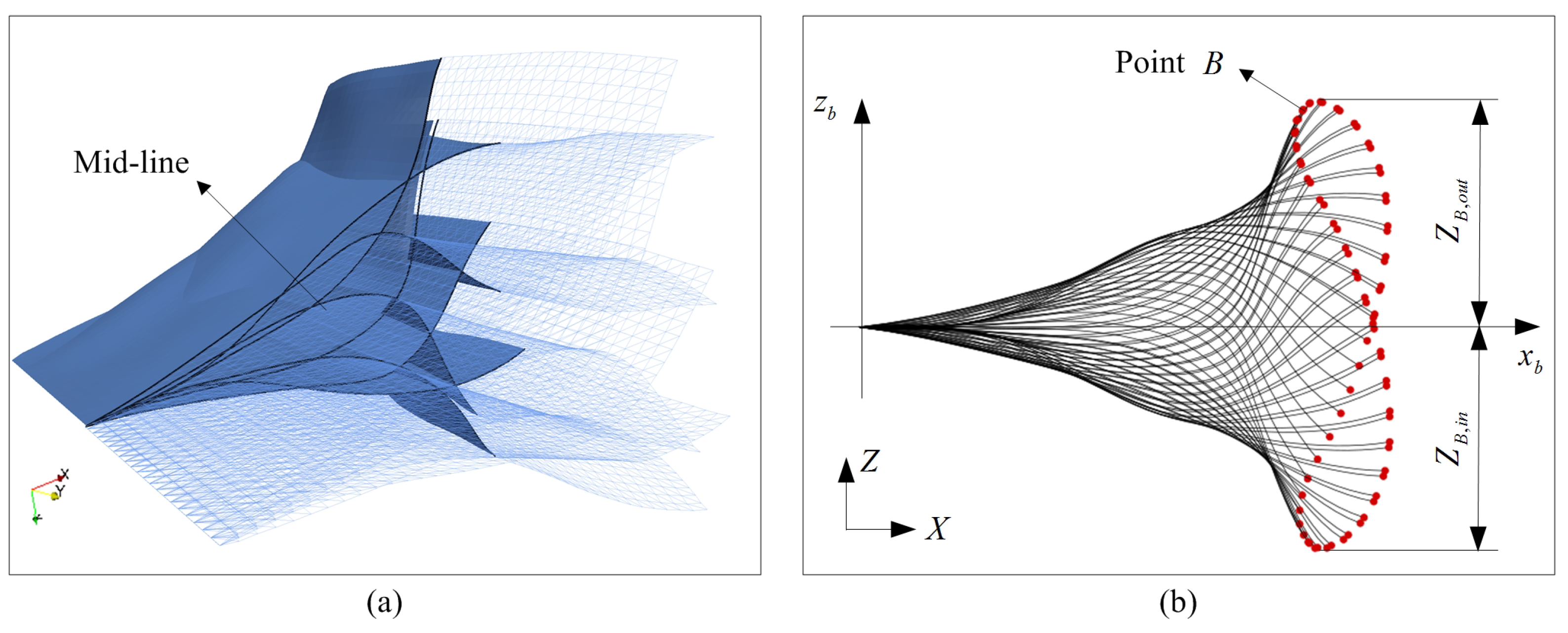
2.1. Physical Problem

A 3D model of the flexible plates in a uniform flow is considered. Figure 1 shows the schematic of flow over two flexible plates in side-by-side arrangement. Both of the two plates are equal in geometry and mechanical property. As shown in Figure 1, the two plates with a fixed leading edge and a free trailing edge are immersed in a uniform flow. The flow’s incoming velocity, dynamic viscosity and density are denoted as $U_{\infty }$, μ and ${\rho }_f$, respectively. In this work, the aspect ratio is finite, defined as $AR=W/L$, where W is the plate’s width and L is the plate’s length. Furthermore, the plate has a density ${\rho }_s$, thickness h and Young’s modulus E. In the initial status, the upper and lower plates keep parallel in the field and have an inclined angle ${\gamma }_0\left({\gamma }_0=\pi /10\right)$ with the streamwise plane. The points $C_1$ and $B_1$ are located on the mid-point of the upper plate’s leading edge and trailing edge, respectively. The line $C_1{B}_1$ is called the upper plate’s mid-line, as well as $C_2{B}_2$ to the lower plate. The transverse gap distance $G_z$ is defined as the distance from point $C_1$ to point $C_2$, denoted as $G_z=\left|C_1{C}_2\right|$. For the purposes of simplification, the non-dimensional parameters L, W and $G_z$ will be used to denote the variants $L/L$, $W/L$ and $G_z/L$, hereafter.

Based on the dimensionless parameters $U_{\infty }$, ${\rho }_f$ and L, the 3D flow field with flexible plates can be described as forced incompressible Navier–Stokes equations [31,32,40]:

$$\frac{\partial \mathbf{u}}{\partial t}+\mathbf{u}·\nabla \mathbf{u}=-\nabla p+\frac{1}{Re}{\nabla }^2\mathbf{u}+{\mathbf{f}}_s$$

(1)

$$\nabla ·\mathbf{u}=0$$

(2)

$$M_s\frac{{\partial }^2\mathbf{X}}{\partial t^2}=\sum _{i,j=1}^2\left[\frac{\partial }{\partial s_i}\left(K_s{\phi }_{ij}\left({\delta }_{ij}-{\left(\frac{\partial \mathbf{X}}{\partial s_i}·\frac{\partial \mathbf{X}}{\partial s_j}\right)}^{-1/2}\right)\frac{\partial \mathbf{X}}{\partial s_j}-\frac{\partial }{\partial s_j}\left(K_b{\gamma }_{ij}\frac{{\partial }^2\mathbf{X}}{\partial s_i\partial s_j}\right)\right)\right]+\mathbf{F}$$

(3)

where ${\mathbf{f}}_s$ is the body force exerted on the fluid by the structure’s boundary. Equation (3) is the plate’s governing equation, which describes its deformation with large displacement [31,32,40]. In this equation, $\mathbf{X}$ is the position of the Lagrangian node on the plate in global coordinates $XYZ$; $K_b$ and $K_s$ are the bending and stretching stiffness of the plate, respectively. $\mathbf{F}$ is the force density acted on the plate’s boundary by the surrounding flow; ${\delta }_{ij}$ is the Kronecker δ function; and ${\gamma }_{ij}$ and ${\phi }_{ij}$ are the out-of-plane and in-plane matrices, respectively.

The mentioned above dimensionless variants concerned in the present model are given as follows:

$$M_s={\rho }_{s}h/\left({\rho }_{f}L\right),K_b=EI/\left({\rho }_f{U}_{\infty }^2{L}^3\right),K_s=Eh/\left({\rho }_f{U}_{\infty }^{2}L\right)$$

(4)

Meanwhile, the Reynolds number in this work is defined based on the plate’s length and incoming flow and can be expressed as:

$$\mathrm{Re}={\rho }_f{U}_{\infty }L/\mu$$

(5)

The drag and lift force are also defined in a dimensionless form, as follows:

$$C_D=F_D/(0.5{\rho }_f{U}_{\infty }^{2}LW),C_L=F_L/(0.5{\rho }_f{U}_{\infty }^{2}LW)$$

(6)

where $F_D$ is the force exerted on the plate in the X-axis direction, while $F_L$ is in the Z-axis direction.

2.2. Numerical Methods

The governing equations of the viscous flow with flexible plates are solved numerically by a hybrid algorithm coupled with the immersed boundary-lattice Boltzmann method and the finite element method. The lattice Boltzmann is adopted to compute the flow field, while the finite element method is applied to compute the structures’ motion. To handle the interactions between plates and surrounding fluid, a four-point-type δ function is introduced.

2.2.1. Mathematical Formulation

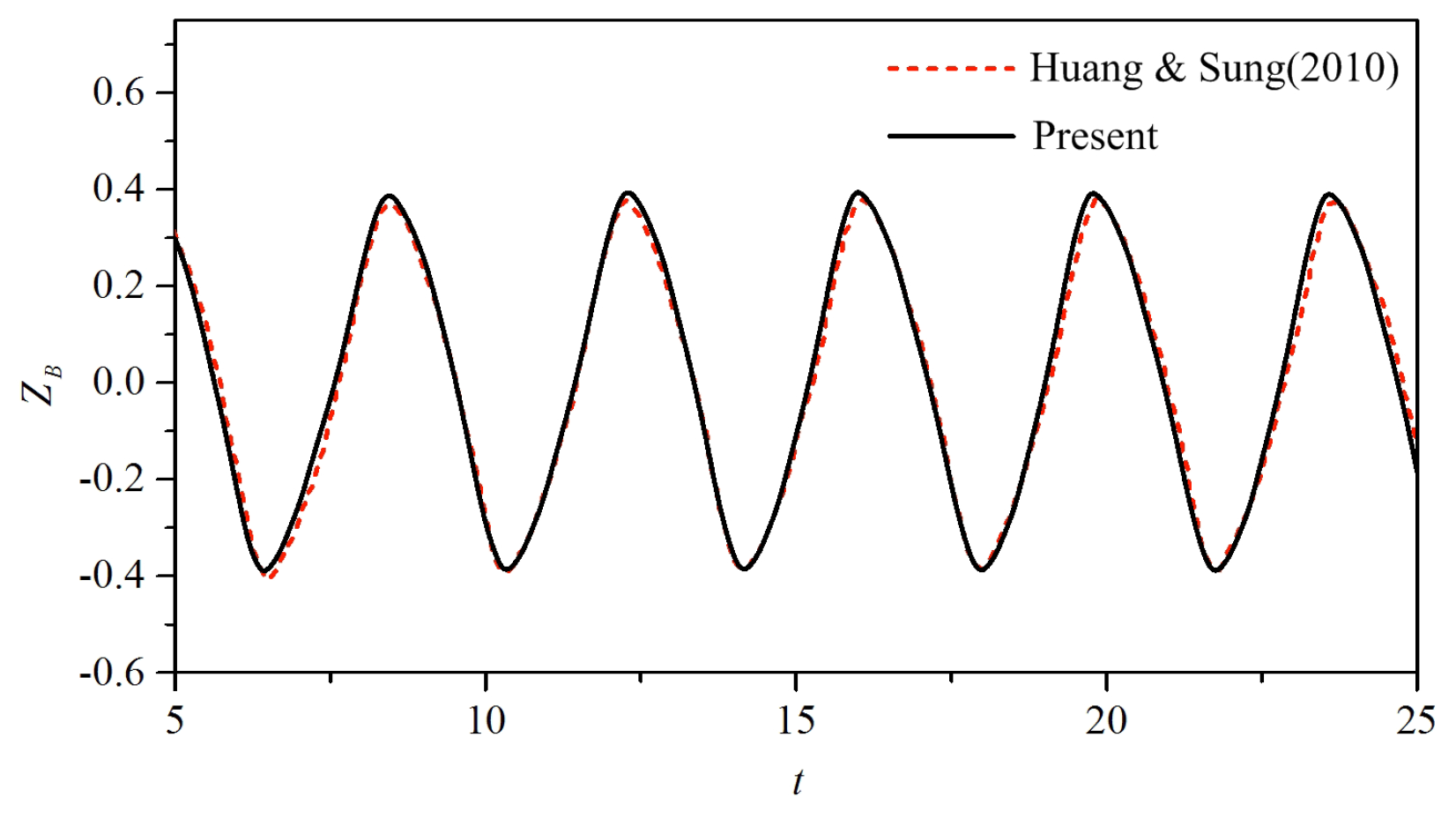
Due to its efficiency and the relative simplicity of the computation, the lattice Boltzmann equation (LBE) with the BGK model has been widely employed to simulate a complex flow field. This method acts as an alternative to the conventional numerical methods in solving Navier–Stokes equations. The BGK-based LBM can be expressed as [35,36,41]:

$$f_i\left(\mathbf{x}+c_i\Delta t,t+\Delta t\right)-f_i\left(\mathbf{x},t\right)=-\frac{1}{\tau }\left(f_i\left(\mathbf{x},t\right)-f_i^{eq}\left(\mathbf{x},t\right)\right)+f_i^F\left(\mathbf{x},t\right)\Delta t$$

(7)

where τ is the dimensionless relaxation time, $\tau =\mu /c_s^2+1/2\Delta t$; $\Delta t$ is the time increment and t is the lattice time step. Additionally, $f_i\left(\mathbf{x},t\right)$ is the distributed function for particles at position $\mathbf{x}$ with velocity ${\mathbf{c}}_i$. The lattice equilibrium distributed function $f_i^{eq}$ and the forcing function $f_i^F$ are given as [42]:

$$f_i^{eq}={\omega }_i\rho \left(1+\frac{{\mathbf{c}}_i·\mathbf{u}}{c_s^2}+\frac{\left({\mathbf{c}}_i{\mathbf{c}}_i-c_s^2\mathbf{I}\right):\mathbf{uu}}{2c_s^4}\right)$$

(8)

$$f_i^F=\left(1-\frac{1}{2\tau }\right){\omega }_i\left(\frac{{\mathbf{c}}_i-\mathbf{u}}{c_s^2}+\frac{{\mathbf{c}}_i·\mathbf{u}}{c_s^4}{\mathbf{c}}_i\right)·{\mathbf{f}}_s$$

(9)

where ${\omega }_i$ is the weighted factor, in the present $D3Q19$ model [36,43], ${\omega }_0=1/3$, ${\omega }_{1-6}=1/18$, ${\omega }_{7-18}=1/36$. Additionally, $c_s$ is the lattice speed of sound. The mass density ρ and fluid velocity $\mathbf{u}$ can be obtained by:

$$\rho =\sum _i{f}_i$$

(10)

$$\rho \mathbf{u}=\sum _i{f}_i{\mathbf{c}}_i+\frac{\Delta t}{2}{\mathbf{f}}_s$$

(11)

With the Dirac delta function in the immersed boundary model, the Lagrangian momentum forcing term is spread to the Eulerian grids, while the Eulerian velocities are interpolated to the Lagrangian meshes; the numerical schemes can be expressed as [36,37]:

$${\mathbf{f}}_s(\mathbf{x},t)=\sum _{s_1,s_2}\mathbf{F}\left(s_1,s_2,t\right){\delta }_{\Delta }\left(\mathbf{x}-\mathbf{X}\left(s_1,s_2,t\right)\right)\Delta s_1\Delta s_2$$

(12)

$$\mathbf{U}\left(s_1,s_2,t+\Delta t\right)=\sum _x\mathbf{u}\left(\mathbf{x},t+\Delta t\right){\delta }_{\Delta }\left(\mathbf{x}-\mathbf{X}\left(s_1,s_2,t\right)\right)\Delta x^3$$

(13)

Based on our careful validations and convergence examinations with different computational sizes and lattice spacings, the computational domain is modeled as a rectangular box, extending from $\left[0,0,0\right]$ to $\left[L_x,L_y,L_z\right]\left(L_x=8,L_y=4,L_z=12\right)$ in the X (streamwise), Y (spanwise) and Z (transverse) directions, respectively. The grid spacing has a uniform value of $\Delta x=\Delta y=\Delta z=0.02$. Here, both the domain size and grid spacing are scaled by the plate’s length L. To simulate the plates’ flap in free stream, the Dirichlet boundary condition $\left(u=U_{\infty },v=0,w=0\right)$ is adopted at the inflow ($x=0$), and a convective boundary condition $\left(\partial \mathbf{u}/\partial t+U_{\infty }\partial \mathbf{u}/\partial x=0\right)$ is applied at the outflow ($x=L_x$). Meanwhile, the far-field boundary condition and periodic boundary condition are used in the transverse ($z=0$ and $z=L_z$) and spanwise ($y=0$ and $y=L_y$) direction, respectively. The fixed boundaries of the plates ($x_b=0$) are aligned with the Y-axis, with their mid-points $C_1$ and $C_2$ located in the mid-plane of the computational domain in the Eulerian coordinate system ($x=L$,$y=1/2L_y$). Each of the plates is discretized using a three-node triangular element [38]. In our simulations, the parameters of ${\phi }_{11}={\phi }_{22}={10}^3$, ${\phi }_{12}=10$, ${\gamma }_{11}={\gamma }_{12}={\gamma }_{22}=0.0001$, $M_s=1.0$, $K_b=0.0001$ and $K_s=1000$ are also taken for the plates by default. Here, the shearing and tension coefficients are taken to be large enough to satisfy the inextensibility conditions for the plates. For the comparison with previous studies, the gravity force is neglected in the present work. All of the computations are implemented at $Re=200$ in this work.

2.2.2. Validation

The validation of the present numerical algorithm will be briefly described in this section. Considering the typical case, we simulate a square $\left(AR=1\right)$ flexible plate in a uniform flow. Compared to the twin plate model shown in Figure 1, there is only an isolated flexible plate immersed in the flow field in this case. Meanwhile, the leading edge of the plate is located in the mid-plane of computational domain $\left(z=1/2L_z\right)$. Figure 2 shows the transverse displacement of the mid-point on the trailing edge; the black solid and red dashed line are the present result and given by Huang and Sung [31], respectively. As it shows, the transverse displacement varies periodically with time increasing, meaning that the plate is flapping passively in the transverse direction. Furthermore, the flapping amplitude of the trailing edge’s mid-point is about 0.77. The present result is almost coincident with the previous studies [31,32,33]. The good agreement indicates that the present numerical algorithm is accurate.

To further analyze the motion of the plate, Figure 3 shows the envelop of an isolated flapping flexible plate, including (a) the 3D envelop of the flapping plate and (b) the envelop of the plate’s mid-line. In the plate’s 3D flapping envelop, the black solid line denotes its mid-line, the segmentation before and after which are displayed in semi-transparent mesh and solid surface style, respectively. As shown in Figure 3a, the plate’s passive flapping is around its fixed leading edge. In the process of passive flapping, the plate loses its initial flat status, which is obviously different from the rigid plate’s flapping [44,45]. Moreover, the motion of the flexible plate apparently contains the deformation streamwise and the deformation spanwise. Due to its flexibility, the plate’s motion in the uniform flow is entirely passive, induced by the interaction between surrounding flow and the structure itself. This deformation characteristic is similar to flapping wings or fins in some extent, especially in spanwise flexibility. According to our previous study [46], the deformation of the tuna’s caudal fin spanwise can improve its propulsive efficiency. Compared to imposing on the fin the prescribed motion equation spanwise, here the deformation is the result of fluid and inertial force, which is much closer to fish swimming in nature. In Figure 3b, point B is the mid-point on the pate’s trailing-edge. The trajectory of point Blooks like the number “8”, which is formed by the free flapping of the plate’s trailing-edge in the transverse direction with the longitudinal traveling wave. Meanwhile, the trajectory of point B is symmetrical about the plate’s local $x_b$-axis, indicating that passive flapping of the plates keeps symmetry in the positive and negative $z_b$-axis direction. Due to the phenomenon of asymmetrical flapping occurring in the side-by-side arrangement, we define $Z_{B,out}$ and $Z_{B,in}$ as the absolute value of the plate’s maximum transverse displacement in the positive and negative $z_b$-axis direction, respectively. Additionally, the flapping amplitude $A_f$ of an isolated plate is defined as $A_f=Z_{B,out}+Z_{B,in}$.

The hydrodynamics and motion of the flexible plate are closely associated with the vortex in the wake. Figure 4 shows the instantaneous vortical structure of flow over an isolated square flexible plate at $Re=200$. Here, the vortical structure is identified by the ${\lambda }_2$ criterion [47], and an iso-surface of ${\lambda }_2=-0.2$ is taken to plot the vorticity contour in 3D. From top to bottom, the three snapshots are chosen at the same instant, but with different projection directions. It can be clearly seen from the figure that a chain of hairpin-like vortical structures is arrayed in order around the flexible plate. In each of the flapping cycles, the vortex formed in the side edges will connect with that formed in the trailing edge when they are moving downstream by the force of inflow. Hence, the connecting vortex actually contains two parts, named the side edge vortex and the trailing edge vortex. Depending on the relative strength of the side edge vortex and trailing edge vortex, the structure behind a plate will show as a double line, hairpin, or ring shaped. Further, it is inferred that the side edge vortex is the main cause of the plate’s deformation in the spanwise direction. Compared to the previous research [31,32], the present study also shows good agreement.

3. Results and Discussion

3.1. Flow around an Isolated Flexible Plate

Figure 5 shows the force and displacement $versus$ aspect ratio $AR$, including (a) mean drag coefficient $\overline{C_D}$ and maximum lift coefficient $C_{L,max}$ and (b) flapping amplitude $A_f$ and Strouhal number $St$. In this study, the aspect ratio is changed from 0.5 to 2.0. As shown in Figure 5a, both the mean drag coefficient and the maximum lift coefficient increase almost linearly with the increasing aspect ratio. As regards the increasing slope, the maximum lift coefficient is clearly higher than that of the mean drag coefficient. This indicates that the maximum lift coefficient is much more sensitive to the aspect ratio. Despite both of the force coefficients monotonically increasing with the aspect ratio, the slopes are less than 1.0. This means that the forces on the plate are not able to increase with the increasing forced area by an equivalent percentage. According to Equation (6), it seems that the force coefficients depend on the plate’s forced area, but actually, the influence of the plate’s geometry shape also has to be considered. As regards the value, the maximum lift coefficient is obviously higher than the mean drag coefficient, and the difference between them also increases with the increasing aspect ratio. This indicates that incoming flow has a stronger influence on the plate in the transverse direction than in the streamwise direction.

As shown in Figure 5b, both the flapping amplitude and Strouhal number increase monotonically with the increasing aspect ratio. Moreover, their increasing slope tends to decrease, which indicates that the effect of aspect ratio on the plate’s flapping amplitude gets weaker as it increases. It is obvious that the two curves are not wholly similar in the increasing trends. Concerning the definition of the Strouhal number, $St=f{A}_f/U_{\infty }$, the flapping amplitude $A_f$ and flapping frequency f are both important influencing factors. Regarding the value, the Strouhal number falls in the range from 0.16 to 0.27 in the present study. Despite the difference in the Reynolds number, the similar values of the Strouhal number were obtained in the simulations of flexible filaments. It is much more interesting that even for an active flapping rigid hydrofoil propelled in a tank, the higher thrust efficiency was found to fall in the range of $0.2\sim 0.4$, which is close to the present study [48]. Furthermore, most fish and birds have been shown to swim or fly near an optimal Stvalue at 0.3 due to the high propulsion efficiency [49]. The similarity in Strouhal number value in animals’ propulsion has been found to be strongly related to the formation of the optimal vortex [50]. These comparisons indicate that wake instability existing in the passive flapping plate is similar to that of swimming fish or flying birds in nature.

The hydrodynamics and flapping motion have close associations with the fluid characteristics. Even if the flow is moving, the relation of fluid-fluid and fluid-structure can be identified to some extent. Figure 6 shows the snapshot of tracing particles from the top and side view, including (a) $AR=0.5$ and (b) $AR=2.0$. The particles are released from the sources at the upstream of the plate with a time interval of 10. It should be noted that the particles’ motion is following the local fluid velocity, but does not affect the fluid motion. As shown in the figure, each pathline of the tracing particle shows a spiral trajectory in the streamwise direction, which is formed in the process of the plate’s flapping. Due to the flexible plate deforming at most instants, the free flapping part of the structure always resists the incoming flow to move downstream in the streamwise direction. Hence, the particle driven by the flow is inclined to separate from the side edge when it encounters the resistance of the trailing edge. This separation behavior consequently induces the plate’s spanwise deformation to some extent. Therefore, the symmetry motion of the tracing particles indicates the symmetry deformation of the plate spanwise. Compared to the results of $AR=0.5$, those of $AR=2.0$ are much more complicated, especially in the knot part of the two pathlines with the same coordinate in the Y-axis direction, as labeled by $k_1$ and $k_2$ in the figure.

Figure 7 shows the instantaneous vortical structures of an isolated flexible plate from the top and axonometric view, including (a) $AR=0.5$ and (b) $AR=2.0$. Both of the cases show a row of a hairpin-like vortical structure arrayed in order behind the plate. The vortical structures are symmetrical about the plate’s centerline, corresponding to the plate’s spanwise deformation. Due to the vortex shedding from the plate being the combination of the side edge vortex and trailing edge vortex, the difference in strength between them has a significant effect on the final combined shape. To observe this difference more clearly, the vortical structures have been labeled as V1 and V2 in the figure, respectively. For $AR=0.5$, the downstream vortical structures are close to a double line shape. This indicates that the plate’s trailing edge vortex has been weakened under the low aspect ratio. For $AR=2.0$, the downstream vortical structures are close to the O shape. This indicates that both of the vortices shedding from the side edges and trailing edge have been strengthened under a high aspect ratio.

3.2. Flow around Two Flexible Plates in Side-by-Side Arrangement

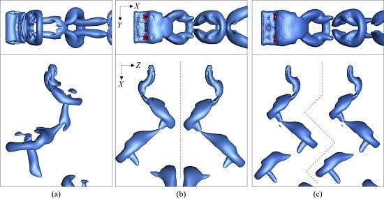
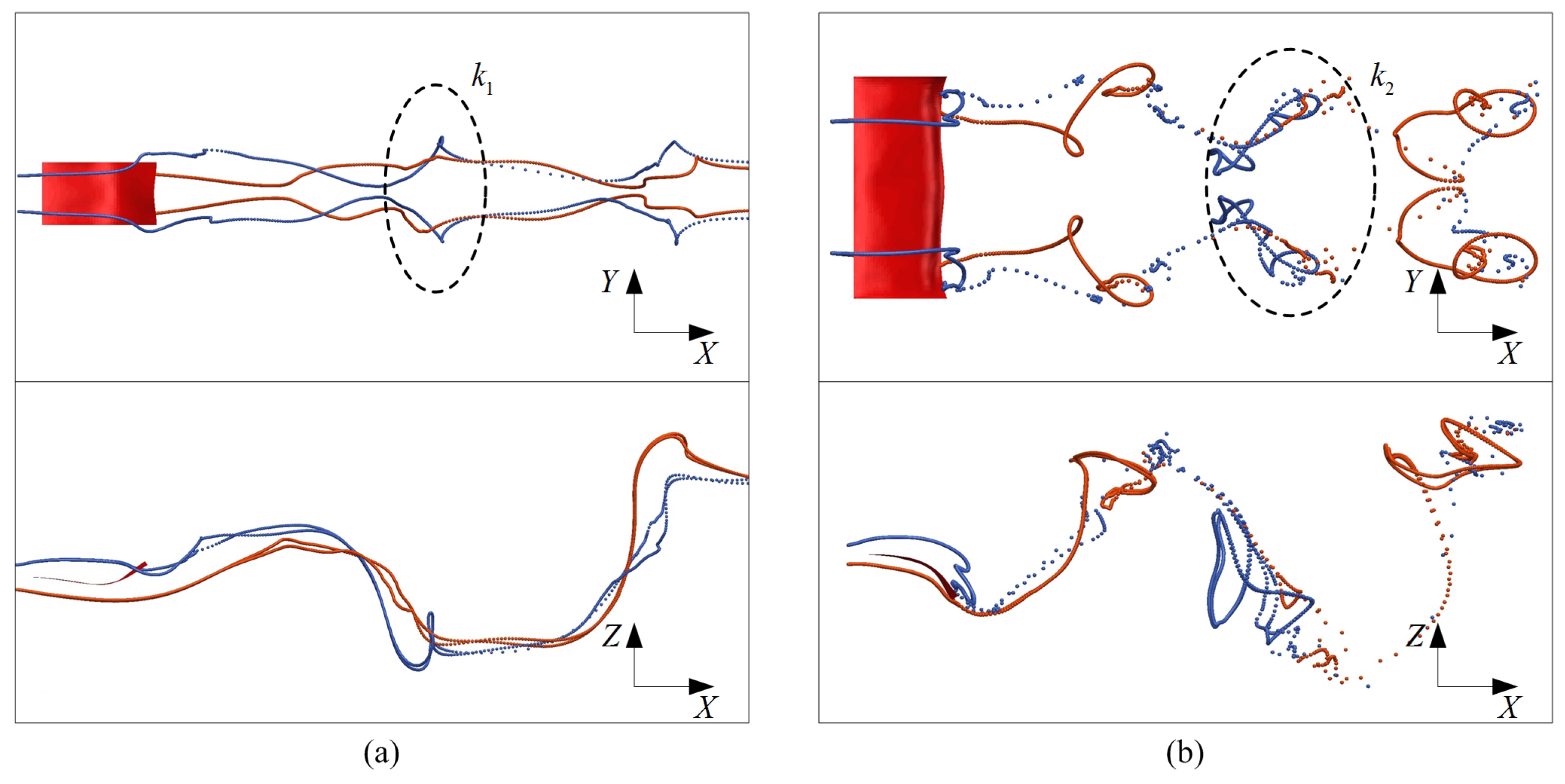
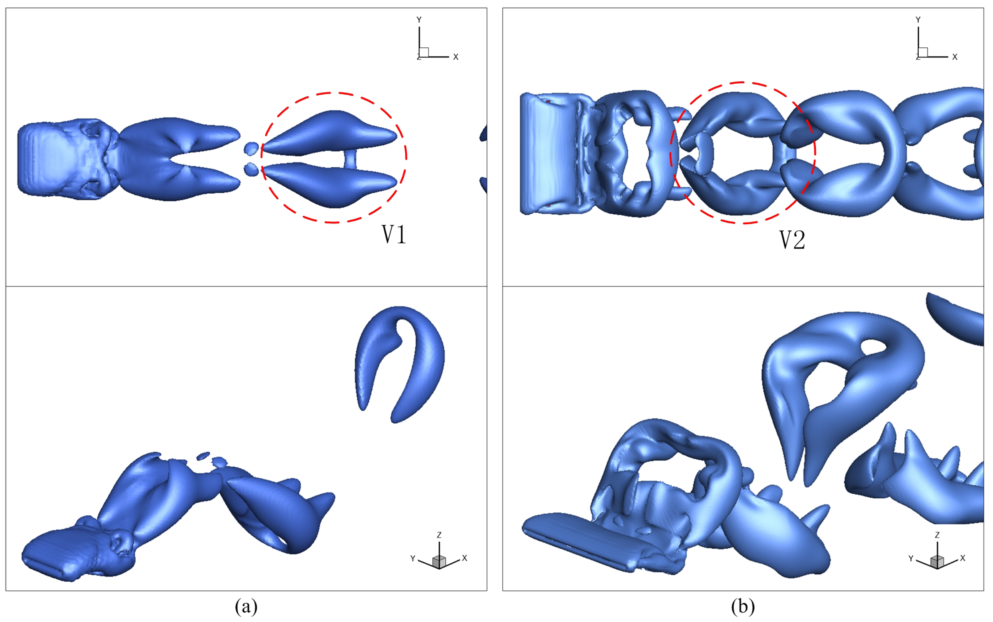
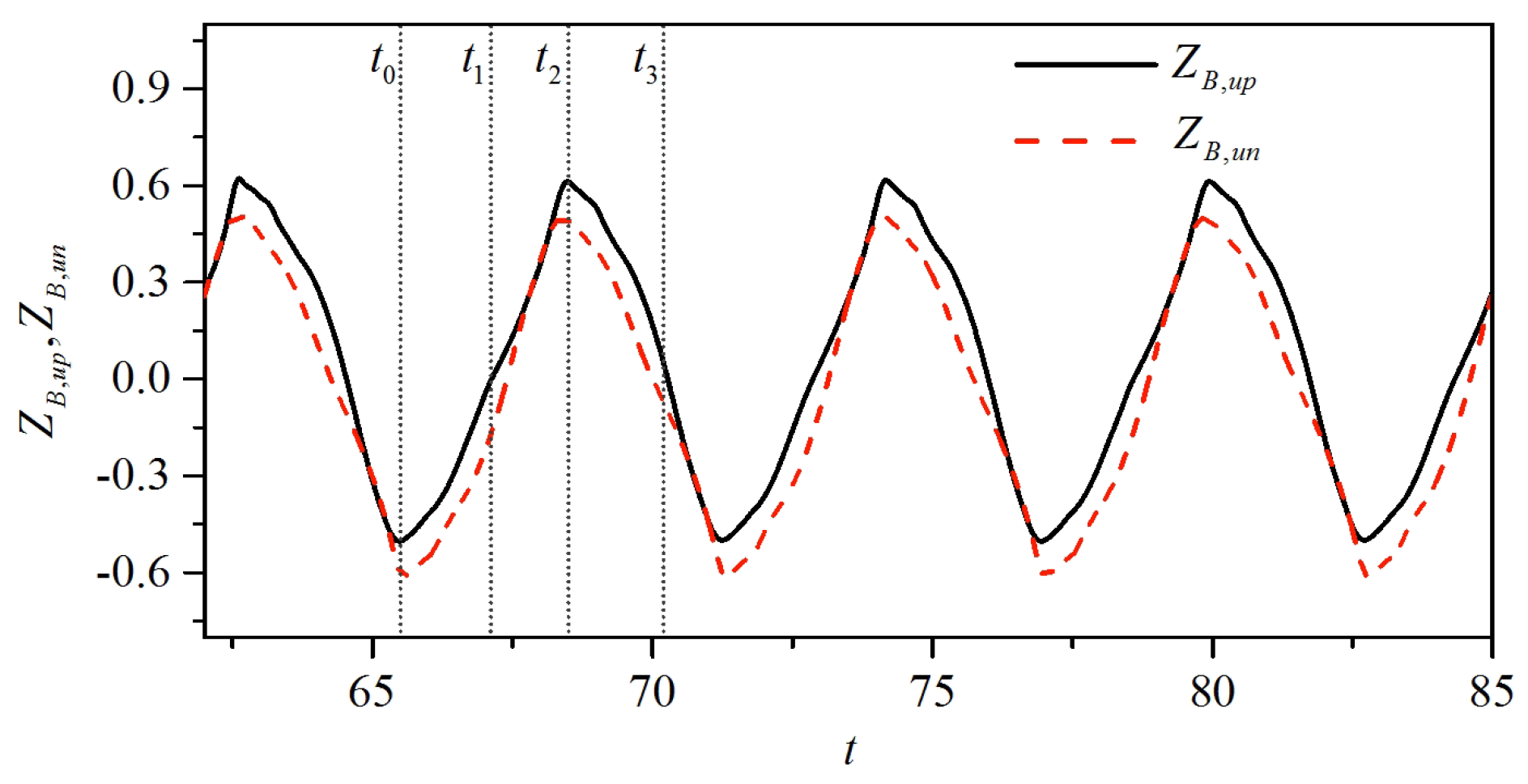
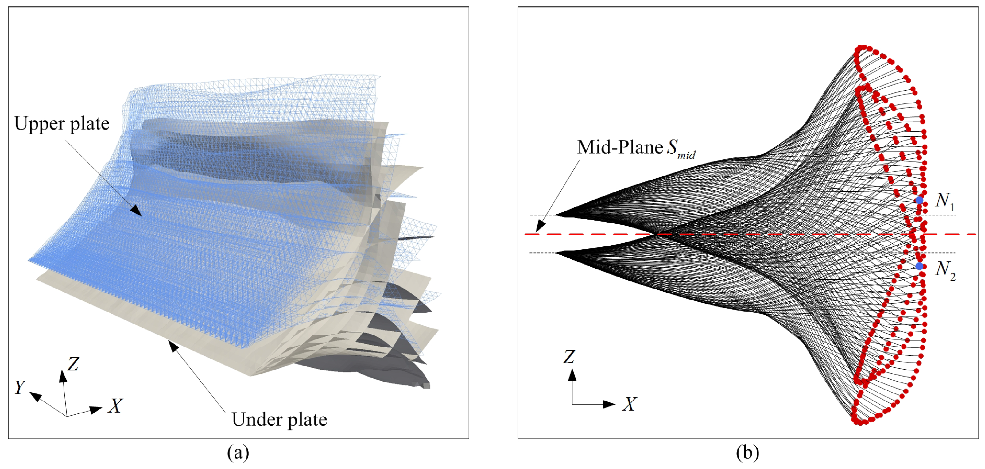
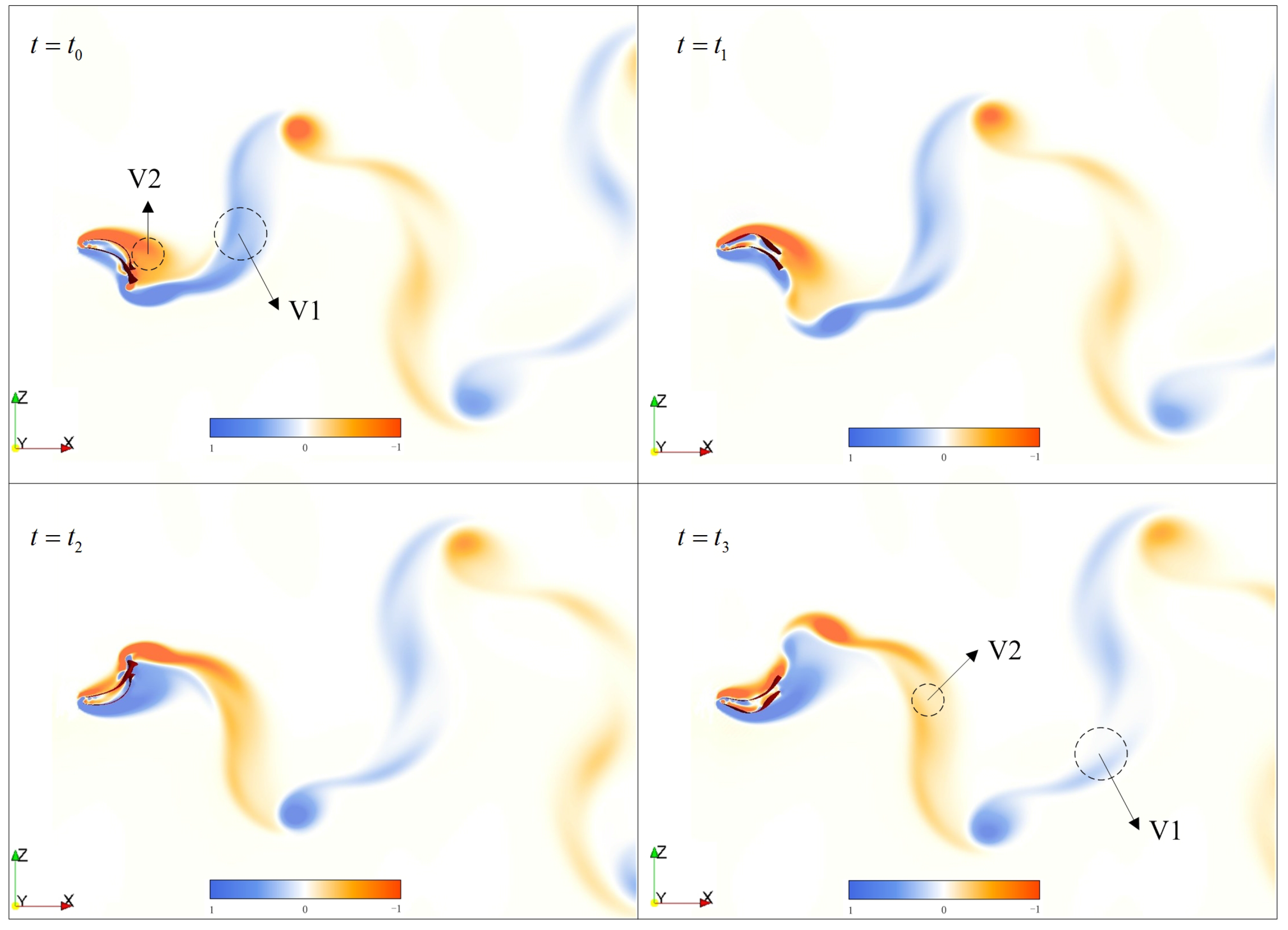
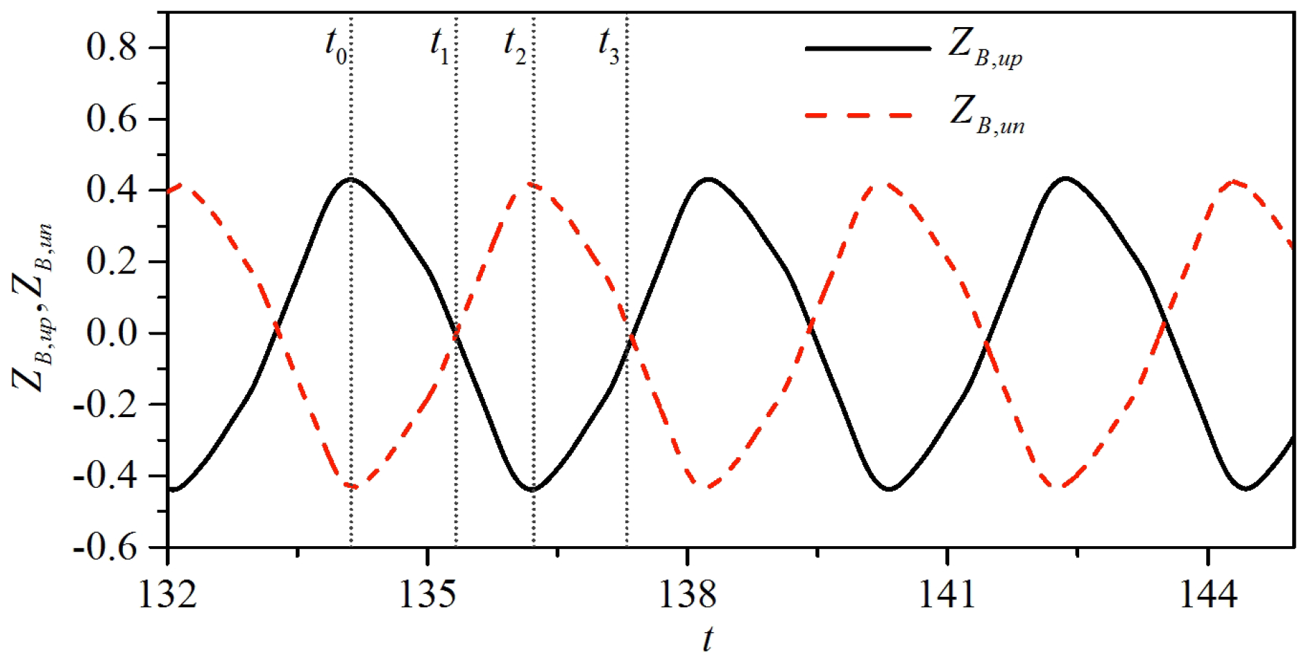
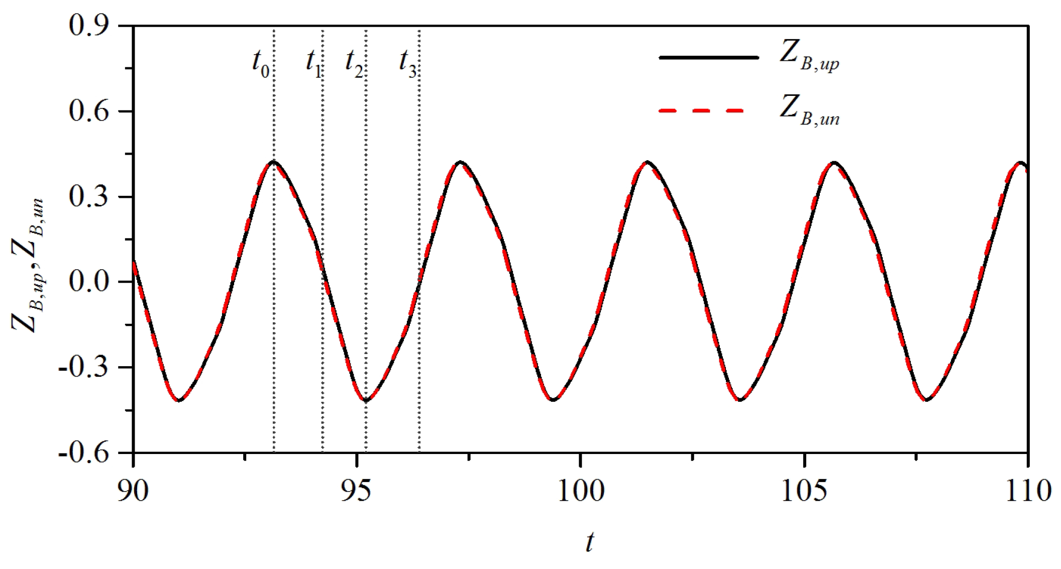
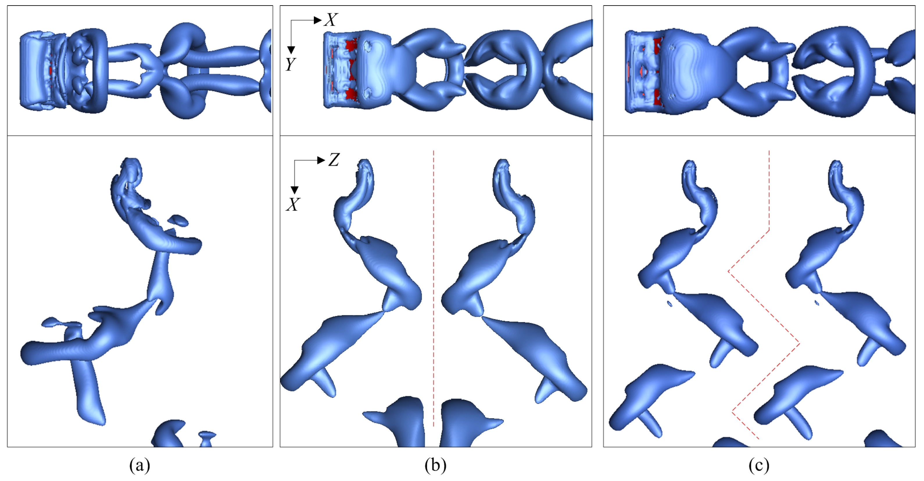
3.2.1. Coupling Motions and Vortical Structures

To understand the interaction dynamics between two flexible plates in a uniform flow, we perform the simulations for side-by-side arrangement. According to the results, the flapping behavior of each plate is asymmetrical about its local $x_b$-axis when the transverse gap distance is small. Meanwhile, the flapping motion of the upper plate is similar to the lower one about the flow domain’s center-plane in the Z-axis direction. For simplicity, the dynamics of the upper plate will be taken for the following description due to their symmetry or similarity. It also should be noted that the following relative flapping amplitude and force coefficient have been scaled by the result of an isolated plate under the same flow condition.

Figure 8 plots the relative flapping amplitude $versus$ transverse distance, including (a) at the outer side and (b) at the inner side. As shown in Figure 8a, $Z_{B,out}$ of the plates under a small aspect ratio ($AR<1.0$) increases monastically with the increasing transverse distance. For instance, as $AR=0.5$, $Z_{B,out}$ increases smoothly and tends to reach the value 1.0. Obviously, $Z_{B,out}$ is less than 1.0 when the two plates are placed nearby, which means that the plates’ flapping is weakened; here, the largest weakened extent is about 10%. However, as the transverse distance increases, $Z_{B,out}$ of the plates under a large aspect ratio ($AR>1.0$) decreases correspondingly until reaching the lowest point, then starts to increase smoothly. For instance, as $AR=1.5$, the value of $Z_{B,out}$ decreases from above the 1.0 level to below the 1.0 level and then starts to increase smoothly. This trend means that the plate’s flapping status transits from strengthened to weakened, and the largest varied extent is about 24% and 5%, respectively. Obviously, the wider (higher aspect ratio) plates can achieve better flapping amplification than the longer plates. In other words, the longer plates in the streamwise direction can achieve better flapping weakened performance in the side-by-side configuration.

As shown in Figure 8b, the trends of $Z_{B,in}$ of the plates under a small aspect ratio are similar to the $Z_{B,out}$. However, the trends of $Z_{B,in}$ of the plates under a large aspect ratio show some differences. Take $AR=1.5$ for instance again; as the transverse distance increases, $Z_{B,in}$ of the plate increases until it reaches the peak. The value of $Z_{B,in}$ is less than 1.0 when the two plates are placed nearby. Recall that $Z_{B,out}$ is increasing, and above 1.0 in this regime, it can be inferred that the flapping motions towards the inside are resisted by the advection in the gap domain. The ratio of $Z_{B,out}$ to $Z_{B,in}$ is always larger than 1.0, and this value gets higher as the aspect ratio increases, meaning that the gap flow has a stronger influence on the wider plates. Despite the difference in various trends, the plates share the common point that the flapping asymmetry phenomenon tends to disappear as the gap distance increases.

Based on a variety of simulations, three distinct coupling modes of the two side-by-side plates are identified depending on the transverse gap distance. Hereafter, the three coupling modes of the plates’ motion are named as single-plate mode, symmetrical flapping mode and decoupled mode, respectively. To clearly introduce the dynamics and interaction mechanisms of these typical motion modes, the plates at $AR=1.5$ are taken as examples. According to the computation results, the parameters at $G_z=0.1$, $G_z=3.0$ and $G_z=4.0$ are corresponding to single-plate mode, symmetrical flapping mode and decoupled mode, respectively. The dynamics of these cases are briefly analyzed as follows.

In the single-plate mode, the two plates are flapping in phase with just a row of vortex existing in the wake. Figure 9 shows the time evolutions of the transverse displacements of points $B_1$ and $B_2$ at $G_z=0.1$. As shown in the figure, the two plates flap synchronously with the same phase. Meanwhile, the two plates’ flapping motion share the equivalent frequency and amplitude. Despite the two displacement curves not overlapping, the peak of $Z_{B,up}$ is equal to the absolute value of minimum $Z_{B,un}$. Therefore, the motion of each plate is asymmetry about its local $x_b$-axis, but the two plates’ flapping amplitude is symmetrical about the flow domain’s transverse center-plane.

Figure 10 shows the envelops of the two flapping flexible plates at $G_z=0.1$, including (a) envelops in 3D and (b) envelops of the plates’ mid-lines. In Figure 10a, the upper and lower plate are displayed in a semi-apparent mesh and a solid surface, respectively. As shown in Figure 10a, the deformation of the upper plate is always similar to the lower one. Additionally, the deformation in the spanwise direction still exists in this situation and keeps symmetrical about the flow domain’s center-plane in the Y-axis direction. As shown in Figure 10b, each of the trailing edge’s mid-point shows an “8” shape trajectory from the side view. The point $N_1$ denotes the intersection node of the trajectory of point $B_1$, so as with point $N_2$ to point $B_2$. It is observed that $N_1$ and $N_2$ are symmetrical about the transverse mid-plane; this result is in accord with Figure 9.

Figure 11 shows the time evolutions of the vortical structures of two side-by-side flapping plates at $G_z=0.1$. The instants $t_0\sim t_3$ in the figure are equal to those in Figure 9. As the plates move towards the positive Z-axis direction, a clockwise vortex gradually forms on the upper surface of the upper plate. As the plates start to move towards the negative Z-axis direction, this fully-developed vortex V2 starts to shed from the trailing edge. Concerning the fluid-induced flapping, the strength of vorticity in both sides of the plates is stronger than in the gap flow; this causes the plate’s asymmetrical flapping motion to some extent. Although there are two flexible plates in the flow domain, just one vortex sheds in half of the flapping cycle. The vorticity pattern in this situation is similar to an isolated plate in the same flow condition, so it is called single-plate mode.

In the symmetrical flapping mode, the two plates are flapping out of phase, and two rows of vortices with opposite rotating directions exist in the wake. Figure 12 shows the time evolutions of the transverse displacements of points $B_1$ and $B_2$ at $G_z=3.0$. As shown in the figure, the two plates flap synchronously, but with the opposite phase. For instance, as the upper plate’s displacement is moving upwards its peak, the lower plate’s displacement is moving downwards its trough at the same time. Each of the plates’ displacements are equal in absolute value, but with the opposite sign. Meanwhile, the two plates’ flapping is periodical and sharing equivalent frequency and amplitude. Clearly, the motion of each plate is symmetrical about its local $x_b$-axis, and the two plates’ flapping is symmetrical about the flow domain’s transverse center-plane.

Figure 13 shows the envelops of the upper flapping plate at $G_z=3.0$, including (a) the axonometric view and (b) the side view. As the plate’s flapping is similar to the other, here just the envelops of the upper one are shown in a semi-apparent mesh. It can be observed that the spanwise deformation still exists in this coupling flapping mode and keeps symmetrical about the flow domain’s center-plane in the Y-axis direction. As shown in Figure 13b, the trailing edge’s mid-point shows an “8” shape trajectory from the side view, as well. Generally, the deformation of the lower plate in this coupling mode is similar to that of an isolated one.

Figure 14 shows the time evolutions of the vortical structures of two side-by-side flapping plates at $G_z=3.0$. The instants $t_0\sim t_3$ in the figure are equal to those in Figure 12. As the upper plate moves downwards (from $t_0$ to $t_2$), a counter-clockwise vortex (labeled V2) forms on the under surface and gradually separates from the trailing edge. During the same time, the lower plate moves upwards, and a clockwise vortex (labeled V1) forms on the upper surface and gradually separates. It is observed the fully-developed vortex shed from one plate will collide with that from the other one. This collision only occurs in the domain away from the trailing edges, so the influence to the flapping motion’s symmetrical characteristic is weak. However, this collision between the opposite vortex will weaken the strength of the separation flow streamwise, then lead to the phenomenon of drag reduction. Considering that the flapping motion and vortex pattern of the plates are symmetrical, we name this coupling status the symmetrical flapping mode.

In the decoupled flapping mode, the two plates are flapping in phase, and two rows of vortex with the same rotating direction exist in the wake. Figure 15 shows the time evolutions of the transverse displacements of points $B_1$ and $B_2$ at $G_z=4.0$. As shown in the figure, the two plates flap synchronously with the same phase. Meanwhile, the two plates’ flapping motions share equivalent frequency and amplitude. Obviously, the two periodical displacement curves almost overlap. Regarding the value of displacement, the flapping motion of each plate is symmetrical about its local $x_b$-axis. The envelops of the upper flapping plate at $G_z=4.0$ are also similar to those of an isolated one (see Figure 3).

Figure 16 shows the time evolutions of the vortical structures of two side-by-side flapping plates at $G_z=4.0$. The instants $t_0\sim t_3$ in the figure are equal to those in Figure 15. As the upper plate moves downwards (from $t_0$ to $t_2$), a counter-clockwise vortex (labeled V2) forms on the under surface and gradually separates from the trailing edge. During the same time, the lower plate moves downwards, as well, and a counter-clockwise vortex (labeled V1) also forms on the under surface and gradually separates from its trailing edge. The two vortexes generated in one-half cycle keep independent without obvious collisions or other interactions. Generally, the flapping motion and vortex pattern of each plate are extremely similar to each other, so it seems like there does not exists any coupling behavior between them. Hence, this coupling status is called the decoupled mode.

From the discussions above, it is obvious that the transverse gap distance can evidently change the flapping dynamics and coupling modes of the two side-by-side flexible plates. The interactions between the two plates are decreasing with the increasing gap distance. According to the characteristics of flapping motion and fluid pattern obtained in the present study, three typical wake modes in such plates’ configuration are classified. The three distinct modes are categorized as single-plate mode, symmetrical flapping mode and decoupled mode, respectively. To show the features more clearly, Figure 17 plots the three typical vortical patterns in the wake of two side-by-side flexible plates. In this figure, the vortical structures are plotted by the ${\lambda }_2$ criterion, including the top view and side view in each subfigure. As shown in the top views ($XY$ plane), all of the plates’ wakes exist in a chain of hairpin-like vortical structures, which are arrayed in order along the streamwise direction. However, the wake patterns are obviously different in the side views ($XZ$ plane). In the single plate mode, the vortex is extremely structured like the result of an isolated plate. In the symmetrical flapping mode and decoupled mode, the two rows of vortical structures are symmetrical and parallel, respectively.

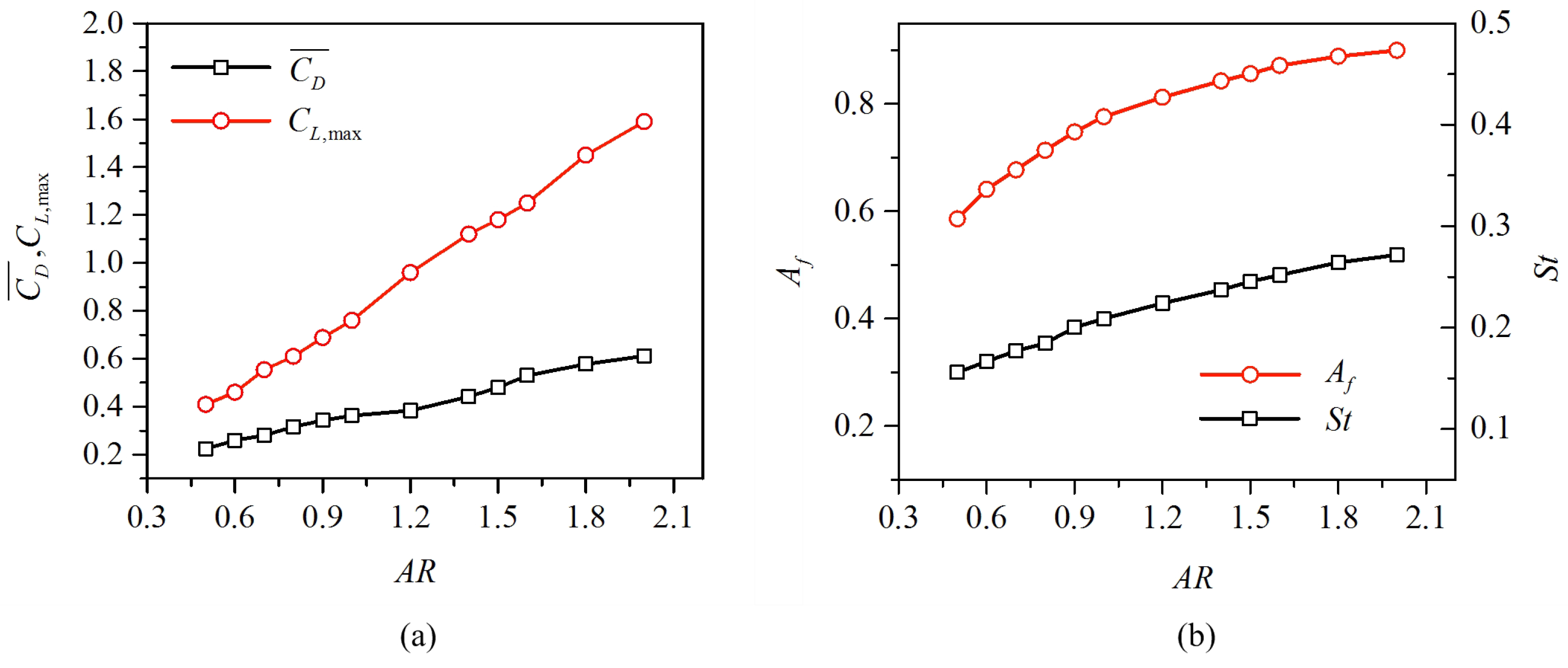
3.2.2. Force and Energy Conversion

The plate’s deformation is associated with the fluid force and energy harvesting performance. Figure 18 shows the relative force coefficient $versus$ transverse distance, including (a) the maximum lift coefficient and (b) the mean drag coefficient. As shown in Figure 18a, the trends of lift amplitude are similar to those of the flapping amplitude. This can be explained briefly by the fact that the plates’ passive flapping is mainly dependent on the lift fore on the boundary. The higher lift force can induce a larger flapping amplitude. As shown in Figure 18b, the trends of the drag coefficient are similar to those of the flapping amplitude, as well, but for different reasons. This can be explained briefly as follows. The drag force on the plate’s boundary is due to the resistance to the incoming flow. This resistance force is proportional to the up-wind area. Hence, the higher amplitude produces a higher projection area vertical to the streamwise, leading to the production of a higher drag force. Regarding the value, the phenomenon of drag reduction is observed when the plates’ aspect ratio is less than 1.0 or the higher aspect ratio plates flap under a large transverse distance.

Here, we examine the relation between coupling modes and energy capture efficiency. Once the plate’s flapping motion is induced by the incoming flow, the deformation is highly dependent on the bending energy captured from the fluid’s kinetic energy. The bending energy $E_b\left(t\right)$ is expressed as:

$$E_b\left(t\right)=\frac{K_B}{2}\int \int \sum _{i,j=1}^2{\gamma }_{ij}\frac{{\partial }^2\mathbf{X}}{\partial s_i^2}·\frac{{\partial }^2\mathbf{X}}{\partial s_j^2}d{s}_{1}d{s}_2$$

(14)

The conversion efficiency from the fluid kinetic energy to the plate’s bending energy can be defined as [51]:

$$\eta =\frac{E_{b,max}}{E_k}=\frac{E_{b,max}}{0.5{\rho }_f{U}_{\infty }^3{Z}_{B,out}W{T}_{out}}$$

(15)

where $E_{b,max}$ is the maximum bending energy at the largest deformation status; $E_k$ is the kinetic energy of the incoming fluid passing through the maximum up-wind area ($Z_{B,out}W$) during a bending phase; $T_{out}$ is the time from when point B crosses the equilibrium position to when it reaches the peak position.

The performance of energy harvesting is shown in Figure 19, including (a) the bending energy and (b) the efficiency of bending energy conversion. In Figure 19a, the red dashed line denotes the result of an isolated plate. It is shown that $E_{b,max}/E_{b0,max}$ of the wider ($AR=1.5$) plate decreases monotonically as $G_z$ increases, while the result of the slender ($AR=0.5$) plate increases monotonically. As $G_z$ increases, both of the results tend to approach the value 1.0. Obviously, the wider plate in side-by-side configuration can capture more energy than in the isolated situation, while the slender plate captures less bending energy. For the purpose of harvesting more bending energy, the optimized selection is the higher aspect ratio plate flapping in the single-plate mode.

In Figure 19b, the η for both of the plates under different $AR$ is decreasing monotonically with $G_z$. Compared to the isolated result, it is found that η is amplified when the plates are placed in the side-by-side configuration. In the present study, the maximum η is 0.57, which is about 32% higher than in the isolated situation. For the purpose of improving the efficiency of bending energy conversion, the plate in the side-by-side configuration is better than in the isolated situation. More specifically, the optimized selection for higher bending energy conversion efficiency is the plate flapping in single plate mode, especially the plate with a higher aspect ratio. To predict the actual energy harvesting performance, the conversion of bending energy to other direct useable energy and its interaction with the plate’s flapping dynamics should be studied, and this is beyond the scope of the present work.

4. Conclusions

The fluid-structure interaction problems of finite aspect ratio flexible plates in a uniform flow have been numerically studied. In the framework of the simulations, the lattice Boltzmann method combined with the immersed boundary and finite element method was used to solve the flow field and the plate’s passive flapping. To compute the equations efficiently in the 3D flow field, the fluid domain was discretized by unifying Cartesian grids, while the structure domain was discretized by Lagrangian grids. To validate this coupled algorithm, the dynamics of flow past a square flexible plate were simulated at low Reynolds number. The results of the validation show good agreements with previous studies by CFD simulations, indicating the efficiency and accuracy of the present method. Then, numerical simulations based on various parameters were carried out, and the mechanisms governing the motions of flexible plates were analyzed systematically. The results related to the plates’ passive flapping dynamics are briefly summarized as follows.

Firstly, the effects of aspect ratio on the fluid-structure interaction dynamics of an isolated plate in a uniform flow have been studied. We have found that the flexible plate can flap periodically with a large amplitude. This passive flapping behavior contains transverse and spanwise deformation. The flexible plate with a larger aspect ratio induced a larger flapping amplitude and Strouhal number. Furthermore, the flexible plate with a larger aspect ratio was subjected to greater drag and lift force. Further, the vortex shed from the side-edge was merged with the one shed from the trailing-edge and formed a hairpin-like structure. The shedding of the side-edge vortex was the main cause for its spanwise deformation.

Secondly, the effects of aspect ratio and transverse gap distance on the hydrodynamics interactions between two side-by-side flexible plates have been studied. With the transverse distance getting higher, we have found three distinct coupling modes of the plates’ motion, including single-plate mode, symmetrical flapping mode and decoupled mode. In the single-plate mode, both of the two plates flapped synchronously, and there was a row of vortex shed from the plates’ system, acting like the characteristic of a single plate in the same flow. In the symmetrical flapping mode, the two plates flapped out of phase, and there was a row of vortex shed form each plate, but with opposite directions. In the decoupled mode, each of the plates flapped synchronously, and there was a row of vortex with the same direction shed from each one, acting like two isolated plates flapping passively in the same flow field. Compared to the flow past an isolated plate, when the plates’ motion was in the single-plate mode, those with a higher aspect ratio got larger flapping amplitudes. Further, the phenomenon of drag reduction was found when the plates’ aspect ratios were less than 1.0 or the higher aspect ratio plates flap in the symmetrical flapping or decoupled mode. For the energy conversion performance, the wider plate in the side-by-side configuration can capture more bending energy than in the isolated situation, while the slender plate captures less bending energy than in the isolated situation. For the purpose of improving the bending energy conversion efficiency, the plate in the side-by-side configuration is better than in the isolated situation. More specifically, the optimized selection for higher bending energy conversion efficiency is the plate flapping in single-plate mode, especially the plate with a higher aspect ratio.

This work has provided several physical insights into the understanding of aquatic animal swimming and is expected to inspire the development of bionic thrusters or renewable energy harvesters. However, the fluid-structure interaction problem in biological propulsion is far more complex and diverse than the model considered here. Future work will focus on the experiments. Furthermore, the hydrodynamic performances of multiple flexible plates with heaving motion in a 3D flow remain to be elucidated.

References

1. Vogel, S. Drag and reconfiguration of broad leaves in high winds. J. Exp. Bot. 1989, 40, 941–948. [Google Scholar] [CrossRef]
2. Tadrist, L.; Julio, K.; Saudreau, M.; de Langre, E. Leaf flutter by torsional galloping: Experiments and model. J. Fluids Struct. 2015, 56, 1–10. [Google Scholar] [CrossRef]
3. Triantafyllou, M.; Triantafyllou, G.; Yue, D. Hydrodynamics of fishlike swimming. Annu. Rev. Fluid Mech. 2000, 32, 33–53. [Google Scholar] [CrossRef]
4. Gazzola, M.; Argentina, M.; Mahadevan, L. Scaling macroscopic aquatic locomotion. Nat. Phys. 2014, 10, 758–761. [Google Scholar] [CrossRef]
5. Lauder, G.V. Fish locomotion: Recent advances and new directions. Annu. Rev. Mar. Sci. 2015, 7, 521–545. [Google Scholar] [CrossRef] [PubMed]
6. Liao, J.C.; Beal, D.N.; Lauder, G.V.; Triantafyllou, M.S. Fish exploiting vortices decrease muscle activity. Science 2003, 302, 1566–1569. [Google Scholar] [CrossRef] [PubMed]
7. Beal, D.; Hover, F.; Triantafyllou, M.; Liao, J.; Lauder, G. Passive propulsion in vortex wakes. J. Fluid Mech. 2006, 549, 385–402. [Google Scholar] [CrossRef]
8. Eldredge, J.D.; Pisani, D. Passive locomotion of a simple articulated fish-like system in the wake of an obstacle. J. Fluid Mech. 2008, 607, 279–288. [Google Scholar] [CrossRef]
9. Lauder, G.V.; Anderson, E.J.; Tangorra, J.; Madden, P.G. Fish biorobotics: Kinematics and hydrodynamics of self-propulsion. J. Exp. Biol. 2007, 210, 2767–2780. [Google Scholar] [CrossRef] [PubMed]
10. Kopman, V.; Laut, J.; Acquaviva, F.; Rizzo, A.; Porfiri, M. Dynamic modeling of a robotic fish propelled by a compliant tail. IEEE J. Ocean. Eng. 2015, 40, 209–221. [Google Scholar] [CrossRef]
11. Giorgio-Serchi, F.; Arienti, A.; Laschi, C. Underwater soft-bodied pulsed-jet thrusters: Actuator modeling and performance profiling. Int. J. Robot. Res. 2016. [Google Scholar] [CrossRef]
12. Ornes, S. Inner Workings: A soft robot that swims like a fish. Proc. Natl. Acad. Sci. 2014, 111. [Google Scholar] [CrossRef] [PubMed]
13. Rus, D.; Tolley, M.T. Design, fabrication and control of soft robots. Nature 2015, 521, 467–475. [Google Scholar] [CrossRef] [PubMed]
14. Cai, Y.; Bi, S.; Zheng, L. Design and experiments of a robotic fish imitating cow-nosed ray. J. Bionic Eng. 2010, 7, 120–126. [Google Scholar] [CrossRef]
15. Moored, K.; Dewey, P.; Smits, A.; Haj-Hariri, H. Hydrodynamic wake resonance as an underlying principle of efficient unsteady propulsion. J. Fluid Mech. 2012, 708, 329–348. [Google Scholar] [CrossRef]
16. Wang, Y.; Tan, J.; Zhao, D. Design and Experiment on a Biomimetic Robotic Fish Inspired by Freshwater Stingray. J. Bionic Eng. 2015, 12, 204–216. [Google Scholar] [CrossRef]
17. Allen, J.; Smits, A. Energy harvesting eel. J. Fluids Struct. 2001, 15, 629–640. [Google Scholar] [CrossRef]
18. Purohit, A.; Darpe, A.K.; Singh, S. Experimental investigations on flow induced vibration of an externally excited flexible plate. J. Sound Vib. 2016, 371, 237–251. [Google Scholar] [CrossRef]
19. McCarthy, J.; Watkins, S.; Deivasigamani, A.; John, S. Fluttering energy harvesters in the wind: A review. J. Sound Vib. 2016, 361, 355–377. [Google Scholar] [CrossRef]
20. Taneda, S. Waving motions of flags. J. Phys. Soc. Jpn. 1968, 24, 392–401. [Google Scholar] [CrossRef]
21. Turek, S.; Hron, J.; Razzaq, M. Numerical benchmarking of fluid-structure interaction between elastic object and laminar incompressible flow. Available online: http://www.mathematik.tu-dortmund.de/lsiii/cms/papers/TurekHron2006b.pdf (accessed on 10 May 2016).
22. Zhu, L.; Peskin, C.S. Simulation of a flapping flexible filament in a flowing soap film by the immersed boundary method. J. Comput. Phys. 2002, 179, 452–468. [Google Scholar] [CrossRef]
23. Connell, B.S.; Yue, D.K. Flapping dynamics of a flag in a uniform stream. J. Fluid Mech. 2007, 581, 33–67. [Google Scholar] [CrossRef]
24. Alben, S.; Shelley, M.J. Flapping states of a flag in an inviscid fluid: Bistability and the transition to chaos. Phys. Rev. Lett. 2008, 100, 074301. [Google Scholar] [CrossRef] [PubMed]
25. Favier, J.; Revell, A.; Pinelli, A. Numerical study of flapping filaments in a uniform fluid flow. J. Fluids Struct. 2015, 53, 26–35. [Google Scholar] [CrossRef] [Green Version]
26. Farnell, D.J.; David, T.; Barton, D. Coupled states of flapping flags. J. Fluids Struct. 2004, 19, 29–36. [Google Scholar] [CrossRef]
27. Alben, S. Wake-mediated synchronization and drafting in coupled flags. J. Fluid Mech. 2009, 641, 489–496. [Google Scholar] [CrossRef]
28. Sun, C.; Wang, S.; Jia, L.; Yin, X. Force measurement on coupled flapping flags in uniform flow. J. Fluids Struct. 2016, 61, 339–346. [Google Scholar] [CrossRef]
29. Daghooghi, M.; Borazjani, I. The hydrodynamic advantages of synchronized swimming in a rectangular pattern. Bioinspir. Biomim. 2015, 10, 056018. [Google Scholar] [CrossRef] [PubMed]
30. Hemelrijk, C.; Reid, D.; Hildenbrandt, H.; Padding, J. The increased efficiency of fish swimming in a school. Fish Fish. 2015, 16, 511–521. [Google Scholar] [CrossRef]
31. Huang, W.X.; Sung, H.J. Three-dimensional simulation of a flapping flag in a uniform flow. J. Fluid Mech. 2010, 653, 301–336. [Google Scholar] [CrossRef]
32. Lee, I.; Choi, H. A discrete-forcing immersed boundary method for the fluid–structure interaction of an elastic slender body. J. Comput. Phys. 2015, 280, 529–546. [Google Scholar] [CrossRef]
33. Zhu, X.; He, G.; Zhang, X. An improved direct-forcing immersed boundary method for fluid-structure interaction simulations. J. Fluids Eng. 2014, 136, 040903. [Google Scholar] [CrossRef]
34. Kim, Y.; Peskin, C.S. Penalty immersed boundary method for an elastic boundary with mass. Phys. Fluids 2007, 19, 053103. [Google Scholar] [CrossRef]
35. Guo, Z.; Shi, B.; Wang, N. Lattice BGK model for incompressible Navier–Stokes equation. J. Comput. Phys. 2000, 165, 288–306. [Google Scholar] [CrossRef]
36. Aidun, C.K.; Clausen, J.R. Lattice-Boltzmann method for complex flows. Annu. Rev. Fluid Mech. 2010, 42, 439–472. [Google Scholar] [CrossRef]
37. Peskin, C.S. The immersed boundary method. Acta Numer. 2002, 11, 479–517. [Google Scholar] [CrossRef]
38. Doyle, J.F. Static and Dynamic Analysis of Structures: With an Emphasis on Mechanics and Computer Matrix Methods; Springer Science & Business Media: Berlin, Germany, 2012; Volume 6. [Google Scholar]
39. Doyle, J.F. Nonlinear Analysis of Thin-Walled Structures: Statics, Dynamics, and Stability; Springer Science & Business Media: Berlin, Germany, 2013. [Google Scholar]
40. Hua, R.N.; Zhu, L.; Lu, X.Y. Dynamics of fluid flow over a circular flexible plate. J. Fluid Mech. 2014, 759, 56–72. [Google Scholar] [CrossRef]
41. Chen, S.; Doolen, G.D. Lattice Boltzmann method for fluid flows. Annu. Rev. Fluid Mech. 1998, 30, 329–364. [Google Scholar] [CrossRef]
42. Guo, Z.; Zheng, C.; Shi, B. Discrete lattice effects on the forcing term in the lattice Boltzmann method. Phys. Rev. E 2002, 65, 046308. [Google Scholar] [CrossRef] [PubMed]
43. Qian, Y.; d’Humières, D.; Lallemand, P. Lattice BGK models for Navier-Stokes equation. EPL (Europhys. Lett.) 1992, 17. [Google Scholar] [CrossRef]
44. Trizila, P.; Kang, C.K.; Aono, H.; Shyy, W.; Visbal, M. Low-Reynolds-number aerodynamics of a flapping rigid flat plate. AIAA J. 2011, 49, 806–823. [Google Scholar] [CrossRef]
45. Suryadi, A.; Ishii, T.; Obi, S. Stereo PIV measurement of a finite, flapping rigid plate in hovering condition. Exp. Fluids 2010, 49, 447–460. [Google Scholar] [CrossRef]
46. Zhou, K.; Liu, J.; Chen, W. Numerical Study on Hydrodynamic Performance of Bionic Caudal Fin. Appl. Sci. 2016, 6. [Google Scholar] [CrossRef]
47. Jeong, J.; Hussain, F. On the identification of a vortex. J. Fluid Mech. 1995, 285, 69–94. [Google Scholar] [CrossRef]
48. Izraelevitz, J.S.; Triantafyllou, M.S. Adding in-line motion and model-based optimization offers exceptional force control authority in flapping foils. J. Fluid Mech. 2014, 742, 5–34. [Google Scholar] [CrossRef]
49. Taylor, G.K.; Nudds, R.L.; Thomas, A.L. Flying and swimming animals cruise at a Strouhal number tuned for high power efficiency. Nature 2003, 425, 707–711. [Google Scholar] [CrossRef] [PubMed]
50. Dabiri, J.O.; Gharib, M. The role of optimal vortex formation in biological fluid transport. Proc. R. Soc. Lond. B Biol. Sci. 2005, 272, 1557–1560. [Google Scholar] [CrossRef] [PubMed]
51. Kim, D.; Cossé, J.; Cerdeira, C.H.; Gharib, M. Flapping dynamics of an inverted flag. J. Fluid Mech. 2013, 736. [Google Scholar] [CrossRef]
Figure 1. Schematic of the flow over two flexible plates in side-by-side arrangement: (a) axonometric view; (b) side view.
Applsci 06 00141 g001
Figure 2. Comparison of the present result with previous data reported by Huang and Sung [31].
Applsci 06 00141 g002
Figure 3. Envelop of an isolated flapping flexible plate: (a) 3D envelop of the flapping plate; (b) envelop of the plate’s mid-line.
Applsci 06 00141 g003
Figure 4. Vortical structure of the flow over an isolated flexible plate (Supplementary Video S1 is available online).
Applsci 06 00141 g004
Figure 5. Force and displacement v e r s u s aspect ratio A R : (a) mean drag coefficient C D ¯ and maximum lift coefficient C L , max ; (b) flapping amplitude A f and Strouhal number S t .
Applsci 06 00141 g005
Figure 6. Snapshots of the tracing particles from the top and side view: (a) A R = 0 . 5 ; (b) A R = 2 . 0 (Supplementary Videos S2 and S3 are available online).
Applsci 06 00141 g006
Figure 7. Instantaneous vortical structures of an isolated flexible plate from the top and axonometric view: (a) A R = 0 . 5 ; (b) A R = 2 . 0 .
Applsci 06 00141 g007
Figure 8. The relative flapping amplitude v e r s u s transverse distance: (a) outer side; (b) inner side.
Applsci 06 00141 g008
Figure 9. Time evolutions of the transverse displacements of points B 1 and B 2 at G z = 0 . 1 .
Applsci 06 00141 g009
Figure 10. Envelops of the two flapping flexible plates at G z = 0 . 1 : (a) envelops in 3D; (b) envelops of the plates’ mid-lines.
Applsci 06 00141 g010
Figure 11. Time evolutions of the vortical structures of two side-by-side flapping plates at G z = 0 . 1 .
Applsci 06 00141 g011
Figure 12. Time evolutions of the transverse displacements of points B 1 and B 2 at G z = 3 . 0 .
Applsci 06 00141 g012
Figure 13. Envelops of the upper flapping plate at G z = 3 . 0 : (a) axonometric view; (b) side view.
Applsci 06 00141 g013
Figure 14. Time evolutions of the vortical structures of two side-by-side flapping plates at G z = 3 . 0 .
Applsci 06 00141 g014
Figure 15. Time evolutions of the transverse displacements of points B 1 and B 2 at G z = 4 . 0 .
Applsci 06 00141 g015
Figure 16. Time evolutions of the vortical structures of two side-by-side flapping plates at G z = 4 . 0 .
Applsci 06 00141 g016
Figure 17. Three typical vortical patterns in the wake of two side-by-side flexible plates ( A R = 1 . 5 ): (a) single-plate mode ( G z = 0 . 1 ); (b) symmetrical flapping mode ( G z = 3 . 0 ); (c) decoupled mode ( G z = 4 . 0 ) (Supplementary Video S4 is available online).
Applsci 06 00141 g017
Figure 18. The relative force coefficient v e r s u s transverse distance: (a) maximum lift coefficient; (b) mean drag coefficient.
Applsci 06 00141 g018
Figure 19. Performance of energy harvesting v e r s u s transverse distance: (a) bending energy; (b) efficiency of bending energy conversion.
Applsci 06 00141 g019