Review

All About Audio Equalization: Solutions and Frontiers

1
Department of Signal Processing and Acoustics, Aalto University, Espoo 02150, Finland
2
Centre for Digital Music, Queen Mary University London, London E1 4NS, UK
*
Author to whom correspondence should be addressed.
Appl. Sci. 2016, 6(5), 129; https://doi.org/10.3390/app6050129
Submission received: 15 March 2016 / Revised: 15 April 2016 / Accepted: 19 April 2016 / Published: 6 May 2016
(This article belongs to the Special Issue Audio Signal Processing)

Abstract

:
Audio equalization is a vast and active research area. The extent of research means that one often cannot identify the preferred technique for a particular problem. This review paper bridges those gaps, systemically providing a deep understanding of the problems and approaches in audio equalization, their relative merits and applications. Digital signal processing techniques for modifying the spectral balance in audio signals and applications of these techniques are reviewed, ranging from classic equalizers to emerging designs based on new advances in signal processing and machine learning. Emphasis is placed on putting the range of approaches within a common mathematical and conceptual framework. The application areas discussed herein are diverse, and include well-defined, solvable problems of filter design subject to constraints, as well as newly emerging challenges that touch on problems in semantics, perception and human computer interaction. Case studies are given in order to illustrate key concepts and how they are applied in practice. We also recommend preferred signal processing approaches for important audio equalization problems. Finally, we discuss current challenges and the uncharted frontiers in this field. The source code for methods discussed in this paper is made available at https://code.soundsoftware.ac.uk/projects/allaboutaudioeq.

Graphical Abstract

1. Introduction

The term equalizer (EQ) has its origins in early telephone engineering, when high frequency losses over long distances had to be corrected so that the spectrum of the sound at the receiver matched the sound spectrum that was initially transmitted. Ideally, the system’s net frequency response has an equal response to all frequencies, and thus the term ‘equalization.’ Since then, the term has been used for any procedure that involves altering or adjusting the magnitude frequency response.
This paper reviews developments and applications in audio equalization. A main emphasis is on design methods for digital equalizing filters. Although these filters were originally constructed using analog electronics, we want to show how to apply them using Digital Signal Processing (DSP).
To our knowledge this is the first review article on red digital audio equalization which gathers all historical developments, methods, and applications, as well as state-of-the-art approaches. However, in 1988 Bohn wrote an overview of this topic, covering the history and the analog era [1]. Additionally, some audio signal processing books have a section devoted to digital equalizers. For example, Orfanidis has a wide section on Infinite Impulse Response (IIR) filters, which includes parametric equalizers and shelving filters [2]. Zölzer’s textbook has a large and excellent chapter on this topic, covering shelving, peak, and notch filters [3]. Reiss and McPherson’s recent book reviews digital tone control and peak equalizing filter designs, among others, and provides a history of the invention of the parametric equalizer [4].
This review article is organized as follows: Section 2 presents the history of audio equalization, Section 3 focuses on parametric equalizers and shelving filters, Section 4 is devoted to graphic equalizers, Section 5 discusses other audio equalizer designs, Section 6 looks into applications in sound reproduction, and Section 7 addresses applications in audio content creation, such as in music production and mixing. Finally, Section 8 concludes this review. The source code for the methods discussed in this paper and for many of the figures are available online at https://code.soundsoftware.ac.uk/projects/allaboutaudioeq, as described in Appendix.

2. History of Audio Equalization

The concept of filtering audio frequencies was understood at least as far back as the 1870s, and was used in designs for harmonic telegraphs. Telegraph operator keys activated vibrating electromechanical reeds, each one assigned a specific frequency. Filtering at the receiving operator was achieved by tuning a similar reed to the same frequency, so that multiple independent connections could be established over a single telegraph line [5].
Telephone lines were equalized in repeaters using wave filters [6,7] to cancel resonances caused by impedance mismatches or the attenuation of high frequencies in long cables. The response of microphones was flattened by appropriately selecting the resistance and other component parameters [8]. Early equalizers were fixed and integrated into the circuits of audio receivers, and later into phonograph playback systems. The advent of motion picture sound saw the emergence of variable equalization. Notably, John Volkman’s external equalizer design featured a set of selectable frequencies with boosts and cuts, and is sometimes considered to be the first operator-variable equalizer. Tone controls—boost and cut applied to bass and treble—were first introduced for use with gramophones in 1949 [9]. In 1952 Baxandall [10] devised tone controls using potentiometers as opposed to switches, thus allowing full user control.
In the 1950s, equalization circuits became a standard part of LP disc production and playback systems. The Recording Industry Association of America (RIAA) proposed a pre-emphasis equalization curve for recording and its complementary de-emphasis equalization curve for playback, see e.g. [11]. The purpose of the RIAA pre-emphasis is to reduce the groove width on the disc by suppressing low frequencies while at the same time improving the signal-to-noise ratio of treble by boosting higher frequencies. Similarly, the National Association of Broadcasters (NAB) suggested a playback equalization curve for C cassettes. It boosted frequencies below 1 kHz, using a first order filter having a pole just below the audio range and a zero above 1 kHz, to obtain a mostly flat frequency response during playback [12].
In what is now considered to be a founding work in the field of sound system equalization, Rudmose [13] applied emerging equalization methods to the Dallas Love Field Airport. Advances in the theory of acoustic feedback led to the development of an equalization system with very narrow notch filters that could be manually tuned to the frequency at which feedback occurs [14,15]. Expanding and extending this work, Conner established the theory and methodology of sound system equalization [16].
Throughout the 1950s and 1960s, equalizers grew in popularity, finding applications in sound post-production and speech enhancement. The Langevin Model EQ-251A, a program equalizer with slide controls, was a precursor to the graphic equalizer [1]. One 15-position slider controlled the gain of a bass shelving filter, and the other adjusted the boost or cut of a peak/notch filter. Each filter had switchable frequencies. Cinema Engineering introduced the first graphic equalizer [1]. It could adjust six bands with a boost or cut range of ±8 dB in 1 dB increments. However, with graphic equalizers, engineers were still limited to the constraints imposed by the number and location of frequency bands. Around 1967, Walker introduced the API 550A equalizer in which the gain appropriately changes the bandwidth of the peak or notch. As was typical in early equalizers, this device had a fixed selection of frequencies, and variable boost or cut controls at those frequencies. In 1971, Daniel Flickinger invented an important tunable equalizer [17]. His circuit, known as “sweepable EQ”, allowed arbitrary selection of frequency and gain in three overlapping bands.
In 1966, Burgess Macneal and George Massenburg, who was still a teenager, began work on a new recording console. They conceptualized an idea for a sweep-tunable EQ that would avoid inductors and switches. Soon after, Bob Meushaw, a friend of Massenburg, built a three-band, frequency adjustable, fixed-Q equalizer. When asked who invented the parametric equalizer, Massenburg stated “Four people could possibly lay claim to the modern concept: Bob Meushaw, Burgess Macneal, Daniel Flickinger, and myself... Our (Bob’s, Burgess’ and my) sweep-tunable EQ was borne, more or less, out of an idea that Burgess and I had around 1966 or 1967 for an EQ... three controls adjusting, independently, the parameters for each of three bands for a recording console... I wrote and delivered the AES paper on Parametrics at the Los Angeles show in 1972 [18]... It’s the first mention of ‘Parametric’ associated with sweep-tunable EQ” [4].
Digital audio equalizers emerged in the late 1970s and early 1980s [19,20,21,22], leading to commercial deployment in Yamaha’s 1987 DEQ7 Digital Equalizer, the first DSP-based parametric equalizer. A year later, Roland rolled out its variable digital equalizer, the E-660. Around the same time, important digital equalizer designs appeared: White published design formulas for digital biquadratic equalizing filters [23], and Regalia and Mitra proposed a useful allpass-filter based structure for digital shelving and parametric equalizing filters [24]. Both of these groundbreaking works are based on discretization of analog prototypes. Since then, there has been a proliferation of advances and improvements, including the octave and 1/3-octave graphic equalizer, constant-Q (bandwidth) graphic equalizers, and many other advances discussed throughout this paper.

3. Parametric Equalizers

The parametric equalizer is the most powerful and flexible of the equalizer types. Midrange bands in a parametric equalizer have three adjustments: gain, center frequency, and quality factor Q (or bandwidth). A parametric equalizer allows the operator to add a peak or a notch at an arbitrary location in the audio spectrum. At other frequencies, far away from the peak or notch, the parametric equalizer does not modify the spectral content, as its magnitude response there is unity (0 dB). Adding a peak can be useful to help an instrument be heard in a complex mix, or to deliberately add coloration to an instrument’s sound by boosting or reducing a particular frequency range. Notches can be used to attenuate unwanted sounds, including removing power line hum (50 Hz or 60 Hz and sometimes their harmonics) [25] and reducing feedback [26]. To remove artifacts without affecting the rest of the sound, a narrow bandwidth would be used.
A single section of a parametric equalizer is created from a second order peaking/notch filter, or in certain cases, a first or second order shelving filter for the lowest and highest frequency bands. When multiple sections are used, they are always connected in cascade so that the effects of each subfilter are cumulative on a decibel scale. In this section, we derive the transfer functions for the first and second order shelving filter and for the second order peaking/notch filter.

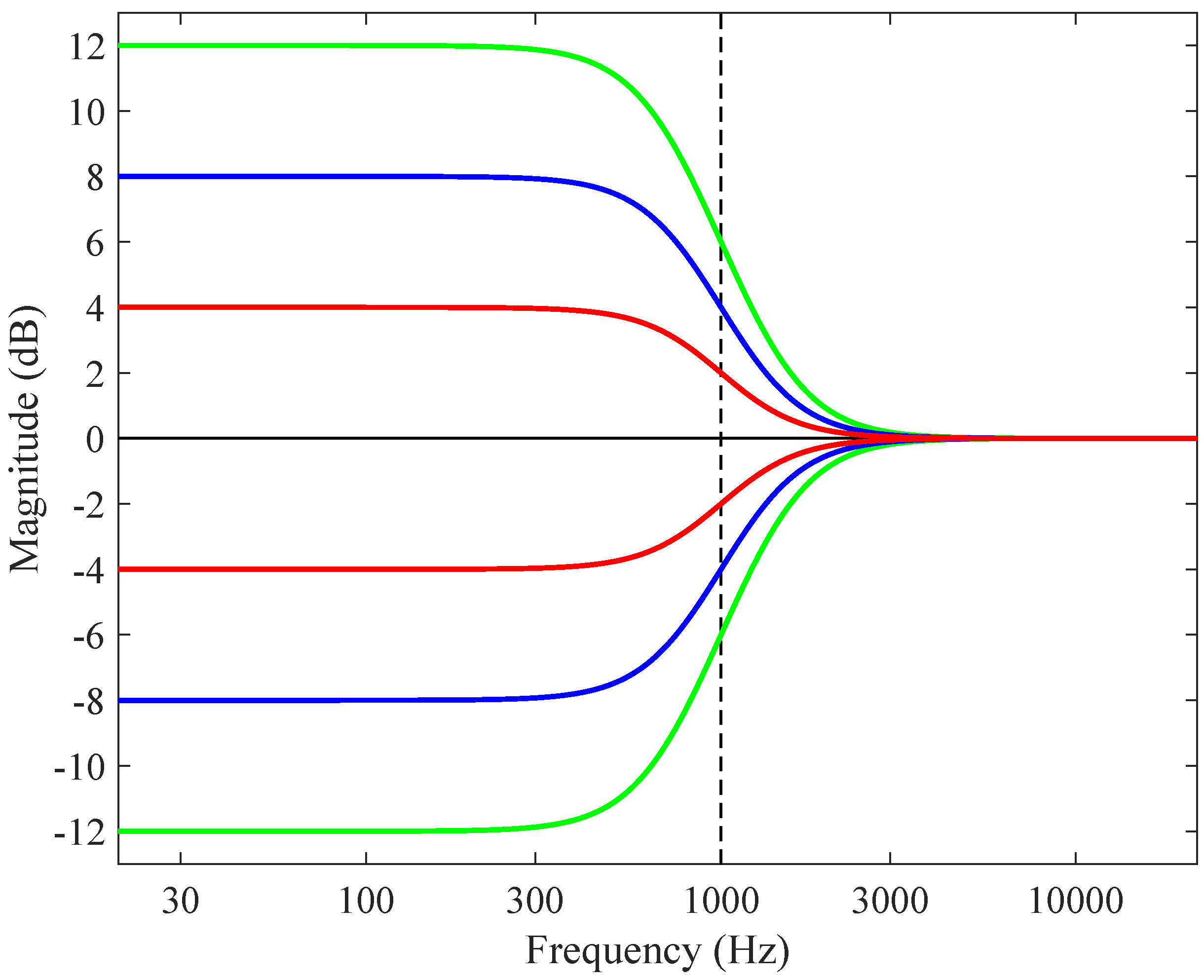
3.1. First Order Shelving Filters

In shelving mode, gain G is applied to all frequencies below or above a crossover frequency f c . These are called the low shelving and the high shelving filter, respectively, and are sometimes used in the lowest-frequency and highest-frequency bands. These shelving filters are similar to those found in the basic tone control, but where the tone control usually uses first order shelving filters, the parametric equalizer uses either first or second order filters. First order shelving filters are used to create smooth transitions (about 6 dB/octave) between affected and unaffected frequency regions. The crossover frequency is sometimes called the corner, cut-off, or transition frequency, but we prefer to use the term crossover herein.
We first derive the transfer function H LS ( z ) for a low-frequency shelving filter. We would like its gain to be G at low frequencies (such as at the zero frequency, or z = 1) and 1 at the highest frequencies (such as at the Nyquist limit, or z = 1 ), that is:
H ( 1 ) = G ,
H ( 1 ) = 1 .
There are several possible choices for the gain at the crossover frequency, such as 3 dB lower (in the boost case) or higher (in the cut case) than the filter gain, e.g., [3,27], but it leads to a confusing situation when the filter gain or loss is smaller than 3 dB [28]. Alternative choices are the arithmetic or geometric mean of the extreme gain factors. However, if the geometric mean is used, then a boost and a cut by the same decibel amount do not cancel. It is also problematic since the arithmetic mean loses its relevance when a decibel scale is used, and it means that the shelving filter will not match the design of peaking and notch filters in parametric equalizers, which often use the geometric mean (see Section 3.3).
We choose to use the midpoint gain G , which corresponds to the geometric mean of the extreme gains (1 and G), and is the arithmetic mean of the extreme gains on a decibel scale. This is one way to retain the overall magnitude response shape when gain G is varied. This requirement may be written as
| H ( e j ω c ) | = G ,
where ω c = 2 π f c / f s is the crossover frequency in radians ( 0 ω c π ), f s is the sampling frequency, and j is the imaginary unit.
We start by defining a prototype low-frequency first order shelving filter, which has its crossover frequency at the midpoint of the frequency range, π / 2 , and has the transfer function of the form
H P ( z ) = g z q z p ,
where p and q are the pole and the zero, respectively, and g is the scaling factor. By evaluating this transfer function at ω c = π / 2 and using the requirement (3), it is seen that a solution is obtained by setting q = p , or by placing the pole and the zero symmetrically w.r.t. the origin on the z plane. The scaling factor must then be g = G :
H P ( z ) = G z + p z p .
The pole location in terms of gain G can be solved by combining Equation (5) and Equation (1):
p = G G G + G ,
which also satisfies Equation (2). Substituting this result to Equation (5) completes the prototype first order low shelf design:
H P ( z ) = G G + G + ( G G ) z 1 G + G ( G G ) z 1 .
To shift the crossover frequency to ω c , which we restrict to be 0 ω c π , we apply the lowpass-to-lowpass transformation [4,29]
z z β 1 β z ,
where
β = 1 tan ( ω c / 2 ) 1 + tan ( ω c / 2 ) .
Rearranging the terms leads to the transfer function of the first order low-frequency shelving filter
H LS ( z ) = G tan ( ω c / 2 ) + G + [ G tan ( ω c / 2 ) G ] z 1 tan ( ω c / 2 ) + G + [ tan ( ω c / 2 ) G ] z 1 .
Due to the choice of gain at crossover frequency, (3), this produces symmetric magnitude frequency responses, above and below the unit gain level, for gains G and 1 / G (i.e., equal boost or cut in dB), as wanted. Figure 1 illustrates this for three pairs of low shelf filters. In this and all other examples, the sample rate is f s = 44,100 Hz and the responses are shown up to the Nyquist limit, f N = 22,050 Hz. When G = 1 , the pole and the zero of the transfer function (10) coincide, the magnitude response becomes unity, and the filter’s impulse response becomes a non-delayed unit impulse.
This way it was possible to derive transfer function coefficients, which are the same for the boost ( G > 1 ) and cut cases ( 0 < G < 1 ), whereas in the past several shelving filter designs have required separate formulas for the two cases, e.g., [3,30,31,32,33]. The transfer function (10) is the same as that given in [4] (Equation (4.1)). Jot recently proposed a modified Regalia-Mitra shelving filter design, which also leads to exactly the same transfer function [34].
The complementary high-frequency shelving filter can be obtained by replacing the gain G in Equation (10) by 1 / G , which yields the inverse filter, and by multiplying the transfer function (numerator) by G, which shifts the magnitude response vertically so that the gain at zero frequency becomes unity (0 dB), and gain G is achieved at high frequencies as desired. Additionally, we multiply both the numerator and the denominator by G to cancel divisions by G:
H HS ( z ) = G tan ( ω c / 2 ) + G + [ G tan ( ω c / 2 ) G ] z 1 G tan ( ω c / 2 ) + 1 + [ G tan ( ω c / 2 ) 1 ] z 1 .
Comparison with Equation (10) shows that these transfer functions are related as H HS ( z ) = G / H LS ( z ) , which means that the pole and the zero of the filter can be interchanged to convert a low shelf to a high shelf or vice versa. Furthermore, a scaling by G must be applied. This implies that a cascade of a low and high shelf with the same crossover frequency ω c and gain G will produce a constant gain G across all frequencies. Figure 2 shows this for a pair of low- and high-frequency shelving filters.
An alternative way to convert a low shelf filter to a high one is to replace z with z in the transfer function (i.e., change the sign of every second coefficient), which turns the response over in frequency so that the zero and Nyquist frequencies are interchanged [28]. Additionally, this low-to-high mapping requires replacing ω c with π ω c to restore the crossover frequency.

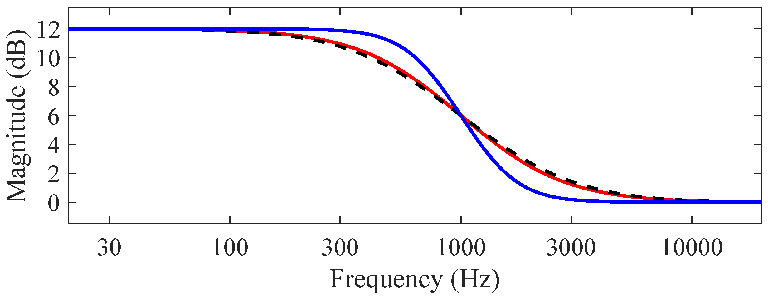
3.2. Second Order Shelving Filters

Here, we show a technique to design a second order low shelving filter, which is often used in parametric equalizer design [19,28,31,32,35]. The design method differs slightly from the approach for first order design since the lowpass to lowpass transformation is performed in the s domain, to keep the maths slightly simpler.
The transfer function of a second order analog shelving filter with crossover frequency f c is given by [3,
H LS , 1 ( s ) = s 2 + 2 G ω 0 s + G ω 0 2 s 2 + 2 ω 0 s + ω 0 2 ,
where s = j ω , ω 0 = 2 π f c , and G is the gain at DC ( ω = 0 ). Note that if the 2 in the numerator and denominator of Equation (12) is replaced with a larger number, then resonant low shelving filters are produced, which have a bump in the magnitude response before the roll-off. The square magnitude of this filter is
| H LS , 1 ( s ) | 2 = G 2 ω 0 4 + ω 4 ω 0 4 + ω 4 ,
so that the square magnitude at the crossover frequency is equal to the arithmetic mean of the square magnitudes at ω = 0 and ω = . However, as discussed in Section 3.1 generally this is not what is wanted. To correct this, we need to find the frequency where the low shelf’s square magnitude is the geometric mean of 1 and G 2 , which is G. So we solve
G = | H LS , 1 ( s ) | 2 = G 2 ω 0 4 + ω 4 ω 0 4 + ω 4 ω = G 1 / 4 ω 0 .
So make the replacement ω G 1 / 4 ω in the low shelf filter, to create a new low shelf H LS , 2 ( s ) . That way, | H LS , 2 ( ω 0 ) | 2 = | H LS , 1 ( G 1 / 4 ω 0 ) | 2 = G . This results in
H LS , 2 ( s ) = ( G 1 / 4 s ) 2 + 2 G ω 0 ( G 1 / 4 s ) + G ω 0 2 ( G 1 / 4 s ) 2 + 2 ω 0 ( G 1 / 4 s ) + ω 0 2 = s 2 + 2 ω 0 G 1 / 4 s + G 1 / 2 ω 0 2 s 2 + 2 ω 0 G 1 / 4 s + G 1 / 2 ω 0 2 .
To convert to the digital domain, we use the bilinear transform. We make the following substitutions
s = z 1 z + 1 , ω 0 Ω = tan ( ω c / 2 ) ,
So
H LS ( z ) = z 1 z + 1 2 + 2 Ω G 1 / 4 z 1 z + 1 + G 1 / 2 Ω 2 z 1 z + 1 2 + 2 Ω G 1 / 4 z 1 z + 1 + G 1 / 2 Ω 2
= G 1 / 2 G 1 / 2 Ω 2 + 2 Ω G 1 / 4 + 1 + 2 ( G 1 / 2 Ω 2 1 ) z 1 + ( G 1 / 2 Ω 2 2 Ω G 1 / 4 + 1 ) z 2 G 1 / 2 + 2 Ω G 1 / 4 + Ω 2 + 2 ( Ω 2 G 1 / 2 ) z 1 + ( G 1 / 2 2 Ω G 1 / 4 + Ω 2 ) z 2 ,
which satisfies all the conditions for the desired low shelving filter. The second order high shelving filter can be derived in the same way, and as with first order shelving filter designs, is equal to the gain G times the reciprocal of the second order low shelving filter:
H HS ( z ) = G 1 / 2 G 1 / 2 + 2 Ω G 1 / 4 + Ω 2 2 [ G 1 / 2 Ω 2 ] z 1 + ( G 1 / 2 2 Ω G 1 / 4 + Ω 2 ) z 2 G 1 / 2 Ω 2 + 2 Ω G 1 / 4 + 1 + 2 [ G 1 / 2 Ω 2 1 ] z 1 + ( G 1 / 2 Ω 2 2 Ω G 1 / 4 + 1 ) z 2
= G / H LS ( z ) .
Figure 3 shows example magnitude responses of the second order low shelving filter. It is instructive to consider whether the second order shelf filter is better than cascading two first order filters. Figure 4 gives an example where we compare the magnitude responses of a single and two cascaded first order shelving filters against that of a second order one. It becomes evident that the second order filter has a steeper transition than the other filters. In fact, cascading two first order filters has a very similar magnitude response as one of them, since the two cascaded filters have a gain of G .

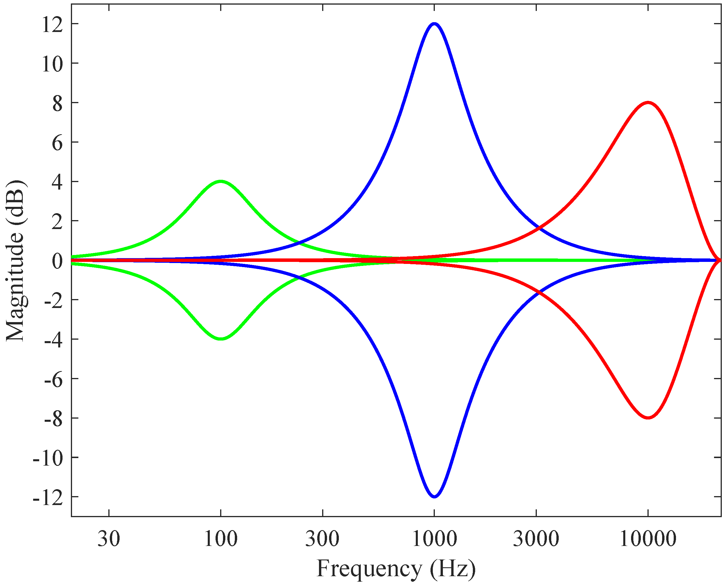
3.3. Second Order Peaking and Notch Filters

In a typical parametric equalizer all sections but the low and high shelving filters are comprised of second order peaking or notch filters, which are IIR filters having two poles and two zeros. The aim is to obtain a filter with the magnitude frequency response, which has a bump of gain G ( G > 1 for a peaking filter and 0 < G < 1 for a notch filter) and width specified by Q at the center frequency ω c , but which has a unity gain (i.e., 0 dB) at frequencies far away from the bump, especially at the zero frequency and at the Nyquist limit. (An alternative approach was taken by Orfanidis who presented a peak/notch filter design in which the specified gain at the Nyquist limit f s / 2 was not unity but the same as that of a corresponding analog equalizing filter [36]. The magnitude responses of his filters are also less asymmetric than the ones designed here, when the center frequency is high, close to the Nyquist limit. See Section 5.2.)
These specifications lead to the following four constraints [37,38] for the filter transfer function H ( z ) :
H ( 1 ) = 1 ,
H ( 1 ) = 1 ,
| H ( e j ω c ) | = G ,
d | H ( e j ω ) | d ω | ω = ω c = 0 .
The bandwidth of the resonance in a parametric equalizer can be defined in one of several ways [2,37]. As with the gain at the crossover frequency of the shelving filter, we choose to define the gain at the upper and lower crossover frequencies ω u and ω l to be equal to G . This leads to the fifth constraint:
| H ( e j ω u ) | = | H ( e j ω l ) | = G .
To shift the crossover frequency to ω c , we set the crossover frequency of our low shelving filter to the bandwidth B of the peaking notch filter,
H LS ( z ) = G tan ( B / 2 ) + G + [ G tan ( B / 2 ) G ] z 1 tan ( B / 2 ) + G + [ tan ( B / 2 ) G ] z 1 ,
and then apply the well-known lowpass-to-bandpass transformation [4,29]
z 1 z 1 z 1 α 1 α z 1 ,
where
α = cos ω c ,
which yields the transfer function of the second order peaking or notch filter:
H PN ( z ) = G + G tan ( B / 2 ) [ 2 G cos ( ω c ) ] z 1 + [ ( G ) G tan ( B / 2 ) ] z 2 G + tan ( B / 2 ) [ 2 G cos ( ω c ) ] z 1 + [ G tan ( B / 2 ) ] z 2 .
The same solution was originally provided by Bristow-Johnson [37] and also recently by Jot [34].
Instead of bandwidth B, peak filters are often parameterized using quality factor Q. These two terms are related by
Q = ω c B .
Figure 5 presents examples of peak and notch filters with fixed Q but varying the other parameters, showing that they are symmetric on the dB scale for G and 1 / G . It is also seen in Figure 5 that when the center frequency is high, such as f c = 10 kHz, the magnitude response itself becomes asymmetric so that the upper skirt (i.e., the magnitude response of a peaking filter on either side of the center frequency) is steeper than the lower one. This feature is caused by the requirement that the digital equalizing filters have a unity gain at the Nyquist limit.

3.4. High Order Filter Designs

In most audio production applications, low order filters are used. The smooth transitions are often advantageous in that the effect of equalization is subtle and not perceived as an artefact. However, they lack the ability for fine control. To address this, higher order IIR filters can be employed. They provide steep transitions at crossover frequencies for shelving filters, or at the upper and lower crossover frequencies for peaking and notch filters.
Orfanidis suggested techniques for the design of high order minimum phase filters based on a variety of classic filters: Butterworth, Chebyshev I, Chebyshev II, and elliptic polynomials [39]. Holters and Zölzer derived high order Butterworth shelving filters [40]. Fernandez-Vazquez et al. focused on the design of such filters based on a parallel connection of two stable allpass filters [41]. Särkkä and Huovilainen modeled analog parametric equalizer responses accurately using high order IIR filters [42]. However, all these high order designs begin with analog prototypes. But it is possible to design high order filters entirely in the digital domain, as described in [4]. We summarize the digital approach next.
Consider a prototype first order, lowpass filter with crossover frequency ω c = π / 2 ;
H ( z ) = 1 + z 1 2 z 1 .
Replace the pole at 0 by N poles given by
p k = j tan ( 2 k N 1 ) π 4 N
and scale the transfer function to again have unity gain at z = 1 . So our Nth order prototype filter becomes
H P ( z ) = k = 1 N 1 2 cos γ k 1 + z 1 j tan γ k + z 1 , where γ k = π [ ( 2 k 1 ) / N 1 ] 4 , with = 1 , 2 , , N .
This filter has the same crossover frequency and same behaviour at DC and Nyquist as the first order filter. But now the poles result in a sharper transition at π / 2 . Then, simple transformations may be applied to each first order section in order to transform this prototype filter into any of the standard designs. The steps to follow in these transformations are depicted in Figure 6.

3.5. FIR Shelving Filter Designs

All types of equalizers discussed herein were originally designed as analog filters, and their digital implementation as IIR filters follows the analog designs as closely as possible. However, FIR (Finite Impulse Response) shelving filters have also been proposed. Lim and Lian [43,44] and Yang [45] applied clever methods to design linear phase FIR shelving filters using long delay lines and a few mathematical operations per output sample. Vieira and Ferreira used a multirate approach to implement the bass shelving filter at one fifth of the audio sample rate while the treble shelving filter was running at the full rate in a linear phase tone control system [46].
Nevertheless, the FIR shelving filter designs have not become popular. One reason is that processing delay is a concern whenever any equalizer is used in live performance. While the maximum allowable total delay in an audio system may be a matter of discussion, it is safe to require each individual device to have the lowest possible processing delay, so as to allow cascading of several devices. This suggests using minimum phase IIR filters instead of linear phase FIR filters, since FIR filters typically exhibit higher latency for the same performance. Another motivation to use minimum phase equalizers is that they emulate more closely the behavior of analog filters.

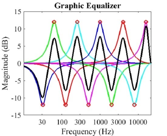
4. Graphic Equalizers

The graphic equalizer is a tool for independently adjusting the gain of multiple frequency regions in an audio signal. Common graphic equalizer designs can provide up to about 30 controls for manipulating the frequency response of each audio channel. Structurally, a graphic EQ is a set of filters, each with a fixed center frequency and bandwidth. The only user control is the command gain, or the amount of boost or cut, in each frequency band, which is often controlled with vertical sliders. The gain of each frequency band can usually be adjusted within the range ±12 dB, corresponding to approximately 0.25 < G < 4 for each filter [19,47,48,49]. The term graphic refers to the fact that the position of the sliders’ knobs can be understood as a graph of the equalizer’s magnitude response versus frequency, which makes the graphic equalizer intuitive to use despite the number of controls. For this reason it is a very popular device for sound enhancement, although it is more restricted than a parametric equalizer. Digital music players, such as those available in mobile phones, usually have several preset settings for the graphic equalizer for different music styles, such as pop, rock, and jazz, see e.g., [50].
A graphic equalizer can be implemented using either a cascade of equalizing filters [21,47,51,52,53] or a parallel bank of bandpass filters [47,54,55,56]. Additionally, hybrid structures have been suggested in which two or more sets of parallel filters are cascaded [57,58]. In a cascade implementation, each equalizing filter determines the magnitude response of the system mainly around its center frequency according to its own command gain, and, ideally, the gain of each equalizing filter should be unity at all other center frequencies to allow independent control of gain on each band. In a parallel implementation, each bandpass filter produces at its center frequency a gain determined by its command gain; the magnitude response of the bandpass filters should be close to zero at all other frequencies to avoid interaction between the filters. Nonetheless, both types of graphic equalizers suffer from interaction between neighboring filters [51,56,59,60]. In practice, a change in one command gain affects the magnitude response on a fairly wide frequency band, and this complicates the design of accurate graphic equalizers. This section first discusses the choice of frequency bands and then continues to the design of cascade and parallel graphic equalizers.

4.1. Bands in Graphic Equalizers

The basic unit of the graphic equalizer is the band. A graphic equalizer typically has more bands than a parametric equalizer. The bands are usually distributed logarithmically in frequency, to match human perception. Let us denote the normalized lower and upper crossover frequencies of the mth band with ω l , m and ω u , m respectively. Bandwidth is the difference between the upper and lower crossover frequencies, B m = ω u , m ω l , m . The frequency bands are adjacent [52], so the upper crossover of band m will be the lower crossover of band m + 1 , ω u , m = ω l , m + 1 . That is, input audio frequencies below this crossover will be primarily affected by the gain control for band m, whereas input frequencies above it will be primarily affected by the gain control for band m + 1 .
The logarithmic distribution of the frequency bands can be specified using a fixed ratio R between each band, so ω l , m + 1 = R ω l , m , ω u , m + 1 = R ω u , m , or B m + 1 = R B m . We also consider the geometric mean of the two crossover frequencies,
ω M , m = ω l , m ω u , m ,
where it can be seen that the same relationship holds for these values, ω M , m + 1 = R ω M , m . Additionally, the bandwidth can be related to the geometric mean ω M , m , because according to Equation (34), ω M , m = R ω l , m = ω l , m / R :
B m = ω u , m ω l , m = R 1 R ω M , m .
Two common designs are octave and 1/3-octave graphic equalizers. An octave is a musical interval defined by a doubling in frequency, so octave graphic equalizers will have the ratio R = 2 between each band. In a 1/3-octave design, each octave contains three bands, which implies R 3 = 2 or R 1 . 26 . So starting at 1000 Hz, an octave spacing would have geometric mean frequencies at 2000 Hz, 4000 Hz, 8000 Hz etc. and a 1/3-octave spacing would have filters centered at 1260 Hz, 1587 Hz, 2000 Hz etc.
The number of bands is determined by their spacing and the requirement to cover the entire audible spectrum. Octave graphic equalizers usually have 10 bands, ranging from about 31 Hz at the lowest to 16 kHz at the highest. Third-octave designs usually have 30 bands ranging from 25 Hz to 20 kHz. These frequencies, shown in Table 1 and Table 2, are standardized by the ISO (International Standards Organization) [61]. Note that some frequencies have been rounded coarsely in the standard in order to have simpler numbers.
The geometric mean of the crossover frequencies of a filter, ω M , m , is not exactly the true center frequency where the filter reaches its maximum or minimum value, ω c , m . We can find a relationship between the upper and lower crossover frequencies and the center frequency of a bandpass, bandstop, peaking or notch filter,
tan 2 ω c , m 2 = tan ω u , m 2 tan ω l , m 2 .
However, the geometric mean is usually quite close to the center frequency. Thus, the bandwidth scales roughly proportionally with the center frequency and higher bands will have a larger bandwidth than lower ones. Since Q = ω c / B , this is another way of saying that the Q factor is nearly constant for each band in a graphic equalizer (such constant Q graphic equalizers were first described in [62]). From Equation (35), we can estimate Q as
Q = ω c , m B m ω M , m B m = R R 1 .
So for an octave equalizer, Q = ω c , m / B m 2 = 1.41, since R = 2. For a third-octave equalizer, Q 2 6 / ( 2 3 1 ) = 4.32, since R = 2 3 .

4.2. Cascade Graphic Equalizers

One way to construct a graphic equalizer is by cascading several peaking/notch filters, as shown in Figure 7, where M is the number of filters. Usually the lowest and highest band filters, H 1 ( z ) and H M ( z ) , are a low and a high shelf filter, respectively [63]. It is possible to include an optional overall gain term G 0 , which may be set to the average or median command gain value [63]. This helps in the cases when many command gains are set to the same value.
The transfer function of the cascade graphic equalizer can be written as
H CGEQ ( z ) = G 0 m = 1 M H m ( z ) ,
where H m ( z ) is the equalizing filter for the mth band ( m = 1 , 2 , , M ). From this form it can be deduced that the total transfer function H CGEQ ( z ) of the cascade structure has all the same poles and zeros as the individual filters H m ( z ) . This implies that when all band filters are minimum phase, the whole graphic equalizer will also have the minimum-phase property. Ideally, each equalizing filter H m ( z ) has magnitude of the desired gain G m inside the band and gain G m at band edges, so that at the crossover frequency, when G m = G m + 1 = G, we have | H m ( e j ω l , m ) H m + 1 ( e j ω u , m + 1 ) | = G . However, in practice other band filters also affect the gain at that frequency, causing interaction, so the total gain may differ from this value.
Figure 8 shows an example magnitude response of a 10-band cascade graphic equalizer. The lowest and highest filters are second order shelving filters designed using Equations (18) and (19), respectively. The rest of the filters are peak/notch filters whose center frequencies have been selected according to Table 1 and bandwidths according to Equation (37) with R = 2 . The bandwidths of band filters H 2 ( z ) to H 9 ( z ) are 44.5 Hz, 88.4 Hz, 176.8 Hz, 353.6 Hz, 707.1 Hz, 1414 Hz, 2828 Hz, and 5657 Hz. The crossover frequency of the low shelf has been chosen to be 46 Hz (instead of 44 Hz, which is the nominal upper band edge frequency) and that of the high shelf is 11,360 Hz, the nominal lower band edge of the highest band (see Table 1).
In Figure 8, the filter gains are set equal to the command gains. Here we neglect the overall gain factor, which is equivalent to fixing it to G 0 = 1 . It is seen that using command gains directly as filter gains leads to severe gain buildup, as the overall magnitude response exceeds the command points. The error is about 5 dB at several center frequencies. This is caused by the skirts of the neighboring band filter responses, which is visible in Figure 8. For example, at 63 Hz (the second command point from the left in Figure 8), the low shelf filter and the 125-Hz peak filter contribute a 2.4 dB and 2.1 dB gain increase, respectively. Additionally, a few other peak filters centered at higher frequencies contribute a few tenths of a dB to that frequency. Together they lead to a 5.0-dB overshoot at 63 Hz. To reduce the overshoot, it seems tempting to change the filter bandwidths to be narrower. In fact, this helps in reducing the gain buildup but increases the ripple by making the valleys between the command frequencies deeper.
The accuracy of a graphic equalizer can be improved by allowing filter gains to be different from command gains, and by then optimizing the filter gains for each command gain configuration. First Abel and Berners [51] and recently Oliver and Jot [63] have proposed to optimize the filter gains of the cascade graphic equalizer by solving a system of linear equations. This is made possible by the fact that the magnitude responses of the peak/notch filters at different gain settings (but with fixed center frequency and Q) are self-similar on the dB scale [51]. (However, Abel and Berners [51] used parametric sections characterized by crossover frequencies at which the filter gain is the square root of its extreme value. Doing so slightly better maintains the self similarity property, as Q varies a little with filter center frequency.)
Thus, the magnitude responses of the peak/notch filters can be used as basis functions to approximate the magnitude response of the graphic equalizer at the center frequencies. This can be written in the form h ^ = Bg , where h ^ is an M-by-1 vector of estimated dB magnitude response values at command frequencies, B is the M-by-M interaction matrix representing how much the response of each band filter leaks to other center frequencies in dB, and g is an M-by-1 vector of command gains in dB,
g = 20 log ( G 1 ) 20 log ( G 2 ) . . . 20 log ( G M ) T ,
where T denotes transposition. The B matrix models the leakage of the filters to other center frequencies when all filter gains are 1 dB [51].
We have estimated the following ten-by-ten B matrix by setting all filter gains of the octave graphic equalizer to 10 dB (an arbitrarily chosen fairly large gain), estimating the dB magnitude response of the filters at the 10 center frequencies, and by dividing the gain values by 10:
B = 0 . 80 0 . 23 0 . 02 0 0 0 0 0 0 0 0 . 19 1 0 . 21 0 . 04 0 . 01 0 0 0 0 0 0 . 04 0 . 21 1 0 . 20 0 . 04 0 . 01 0 0 0 0 0 . 01 0 . 04 0 . 20 1 0 . 20 0 . 04 0 . 01 0 0 0 0 0 . 01 0 . 04 0 . 20 1 0 . 20 0 . 04 0 . 01 0 0 0 0 0 . 01 0 . 04 0 . 20 1 0 . 20 0 . 04 0 . 01 0 0 0 0 0 . 01 0 . 04 0 . 20 1 0 . 20 0 . 03 0 0 0 0 0 0 . 01 0 . 04 0 . 21 1 0 . 18 0 . 01 0 0 0 0 0 0 . 01 0 . 06 0 . 25 1 0 . 10 0 0 0 0 0 0 0 0 . 01 0 . 14 0 . 94 .
Using the inverse matrix of B , it is now possible to determine the filter gains g opt which approximate in the least squares sense the magnitude response specified by command gain values g [51]:
g opt = B 1 g .
The inverse matrix B 1 can be computed off-line and then stored. It is applied every time a command gain is changed. This means that all filter gains will be modified even if one command gain is changed, and so all band filters must also be redesigned using Equation (29).
Figure 9 shows an example usage of the above method. The gain of all peak filters is about 6 dB although all command gains are at 10 dB, because the modeling technique accounts for the gain buildup caused by interaction. The overall magnitude response of the graphic equalizer is, however, quite close to the command points. The maximum error, which occurs at the 125-Hz point, is only 0.5 dB—a remarkable improvement over the example of Figure 8. Nevertheless, the overall fit is not highly accurate, because the response still oscillates between the command points. The peak-to-peak extent of this ripple (about 2 dB in this case) is proportional to filter gains. Oliver and Jot [63] mitigated this issue by setting the global gain G 0 to the median of all command gain values and offsetting these values accordingly.
To reduce the ripple in a cascade graphic equalizer’s magnitude response, Azizi [59] has proposed to use extra filter sections, which he calls ‘opposite’ filters, between the band filters in a cascade graphic equalizer. When the gain and Q value of the opposite filters are set appropriately, the ripple seen in the overall response can be reduced further. Lee et al. refined this method by allowing the Q value of the band filters to change with gain [64]. McGrath et al. developed an accurate graphic equalizing method by constructing each band filter using several cascaded second order filters so that its magnitude response approximates a cosine pulse, spanning one band only [65]. Such high order filters have reduced interference, while the overall computational cost of the graphic equalizer is increased. Chen et al. have proposed an optimization method, which needs good initial values and definition of the desired gain at command points as well as at additional intermediate frequency points and which then iteratively adjust the coefficients of the cascaded biquad filters to reduce the mean squared error [66].
Holters and Zölzer showed how cascaded high order equalizing filters can be effectively used in graphic and parametric equalizer design [52]. Each high order band filter has a steep roll-off at its crossover frequencies, so the interference between bands gets reduced in comparison to an equalizer based on second order band filters. Even a graphic equalizer based on fourth order band filters is considerably more accurate than the one based on second order filters, as the examples shown in [56] demonstrate. Rämö and Välimäki presented a filter optimization algorithm for the high order graphic equalizer, which minimized errors in the transition bands by iteratively optimizing the orders of adjacent band filters [53].

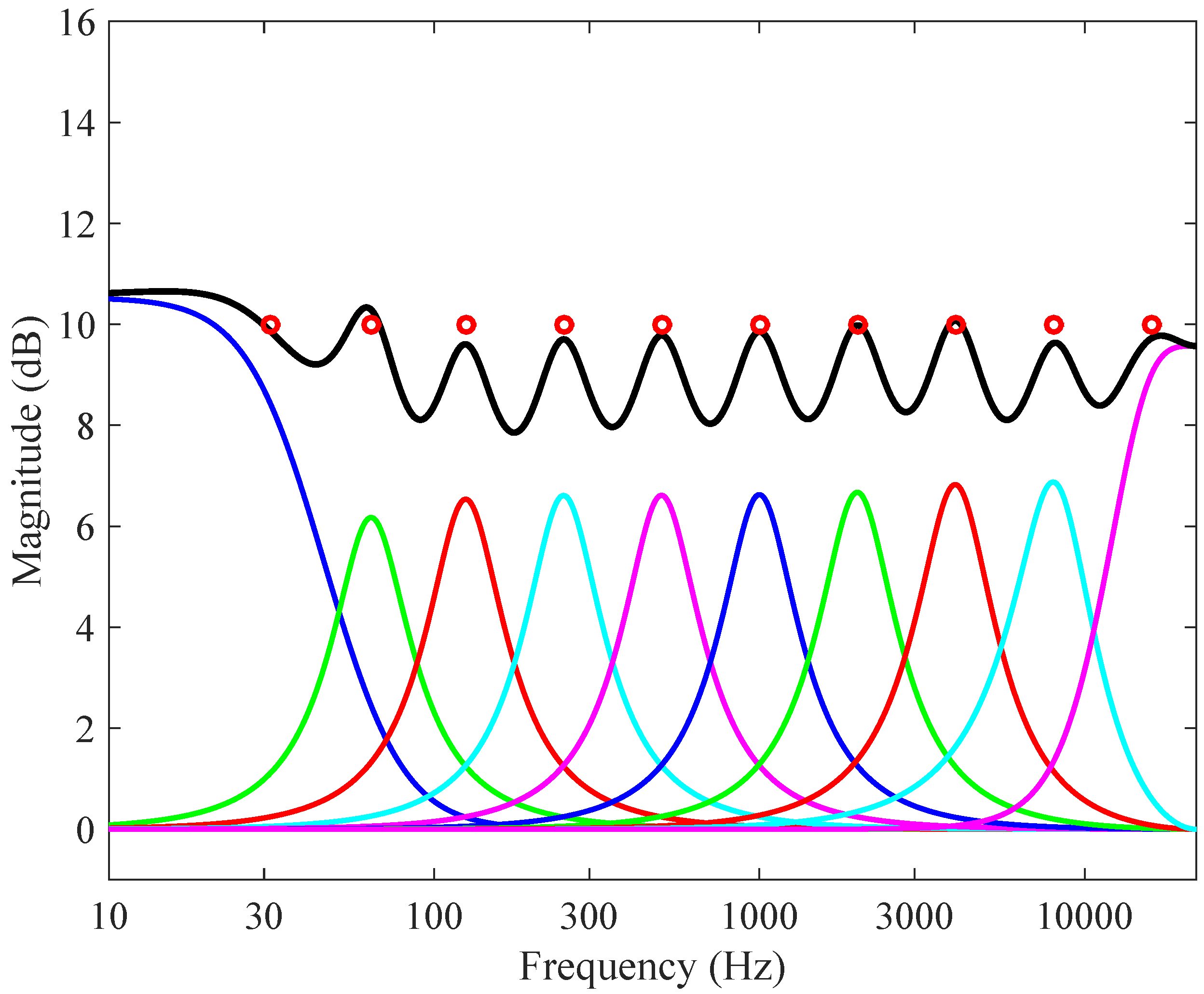
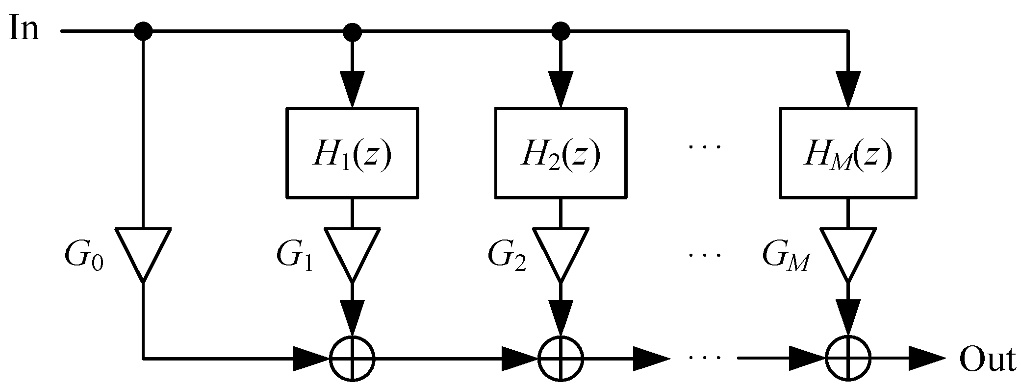
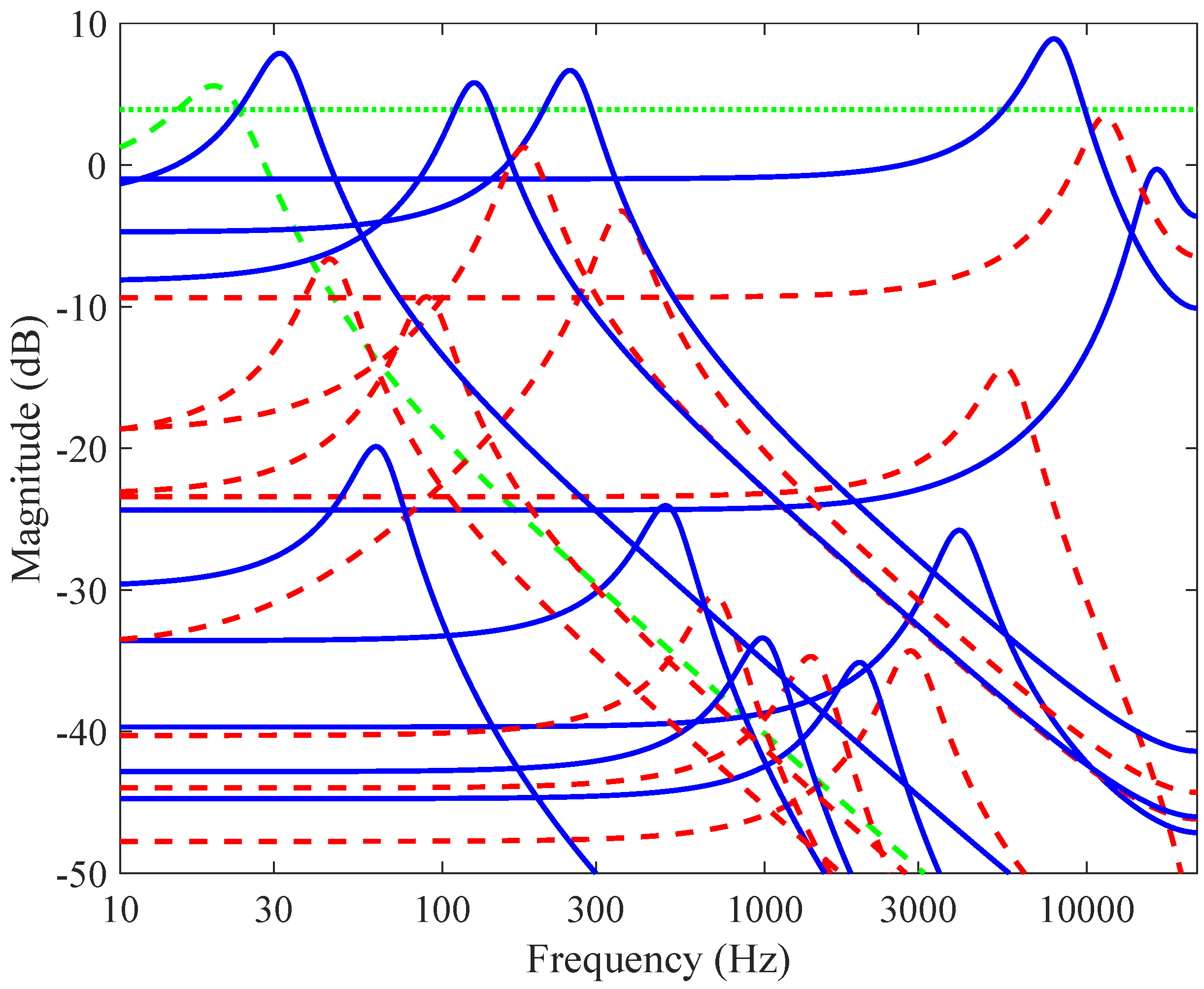
4.3. Parallel Graphic Equalizers

Instead of using a cascade structure, a graphic equalizer often uses a collection of bandpass filters arranged in parallel, as shown in Figure 10 [47,54,55,56]. The audio input is split and sent to the input of every bandpass filter. It is common to include a direct path, which passes the scaled input signal to the output, as seen in Figure 10. Each filter allows only a narrow frequency band to pass through. Ideally, the center frequencies and bandwidths are configured so that if all the outputs were added together, the original signal would be reconstructed. The controls on the graphic equalizer are then implemented by changing the gain of each bandpass filter output before the signals are summed together. In theory, the parallel and cascade implementations are mathematically identical but their design must be treated differently. Parallel connection of bandpass filters avoids the accumulating phase errors and, potentially, quantization noise, found in the cascade. The parallel filter structure is also well suited to parallel computing [67].
In the parallel structure, the direct path with gain G 0 allows easy implementation of flat command gain configurations, just like in the cascade structure. For example, the constant 10-dB gain at all command bands, which was shown in Figure 8 and Figure 9, can be easily implemented using the parallel graphic equalizer by setting G 0 = 3 . 2 and by zeroing all other filter gains. However, the parallel structure is equally prone to interaction between band filters as the cascade structure, when command gains are set to a non-flat configuration. The transfer function of the parallel graphic equalizer is obtained as the sum of all band filters and the direct path:
H PGEQ ( z ) = G 0 + m = 1 M G m H m ( z ) .
This implies that also the phase, not only the magnitude response, of each bandpass filter affects the total frequency response of the parallel graphic equalizer. Therefore, for good accuracy it is necessary to optimize the gain and phase of all filters for each command gain setting. This is inevitably more complicated than design of a cascade structure.
Rämö et al. recently developed a parallel graphic equalizer, which can accurately follow the command gain settings [56]. This method is based on Bank’s fixed-pole parallel filters [68,69]. In this structure, each IIR filter transfer function H m ( z ) has a second order denominator but a first order numerator:
H m ( z ) = b m , 0 + b m , 1 z 1 1 2 | p m | cos ( θ m ) z 1 + | p m | 2 z 2 , for m = 1 , 2 , , M ,
where p m and θ m are the pole radius and pole angle of the mth bandpass filter. The poles are set in advance at pre-designed frequencies determined by the frequency resolution of the graphic equalizer. When an octave graphic equalizer is designed, the poles are set at the 10 standard frequencies from 31.5 Hz to 16 kHz, which are listed in Table 1. To obtain high accuracy, additional poles are assigned between each two standard center frequencies (at their geometric mean frequency) and below the lowest standard frequency (for example at 20 Hz), so that there will be altogether 20 predesigned poles. The pole radii are chosen so that the magnitude responses associated with neighboring poles meet at their 3 -dB points:
p m = e Δ θ m 2 e ± j θ m ,
where Δ θ m are the differences between the neighboring pole frequencies [56].
This graphic equalizer design uses least squares optimization to adjust the direct path gain G 0 and the numerator coefficients b m , 0 and b m , 1 for each filter. This method requires a target frequency response H t ( ω k ) to be constructed by interpolating between the points defined by the command gains. Hermite interpolation has been shown to be suitable for this, as it does not introduce overshoot [56]. A computationally efficient method combining linear interpolation and constant segments reduces the computational complexity of this design without much reduction in the accuracy [70]. For good accuracy, the target response needs to be evaluated at 10 times as many points as there are pole frequencies [56].
In addition to the target magnitude response, the target phase response must be generated. A natural choice for a graphic equalizer is a minimum phase response. This requires resampling the target response to the linear frequency scale and computing the Hilbert transform of the log magnitude response using FFT and IFFT operations. In the end, the data is sampled again at logarithmic frequency points.
A modeling matrix M is constructed by sampling the complex frequency responses of the denominators and their delayed versions. A non-negative weighting function W ( ω k ) = 1 / | H t ( ω k ) | 2 is needed to ensure that attenuation is implemented as accurately as amplification [56]. Finally, the optimal parameters p opt are obtained as
p opt = ( M H WM ) 1 M H Wh t ,
where M is the modeling matrix, M H is its conjugate transpose, W is the non-negative diagonal weighting matrix, and h t is the column vector containing the target response. As a result, every time a command gain is changed, both the target response and the weighting matrix also change and matrix inversion needs to be executed [56].
Figure 11 shows a design example in which the command gains are set to ± 10 dB. For the octave equalizer, the target response was interpolated at 100 points on the logarithmic frequency axis from 20 Hz to 22,050 Hz. Now the match to the command points is excellent. The largest deviation at a command point is 0.64 dB, which occurs at the lowest point 31.5 Hz.
Figure 12 illustrates the subfilters used to obtain this result. It is interesting to see that even the gains of the main filters having a pole at command frequencies (blue solid lines) do not coincide with the command gains, but are smaller. The intermediate (dashed red lines) filters usually have a gain midway between the neighboring main filters. Additionally, the responses related to the extra pole at 20 Hz and the direct path gain (3.9 dB) are shown. Since only magnitude responses of the subfilters are shown, Figure 12 fails to illustrate the effects of phase.
The computational load of the above parallel graphic equalizer is modest: its operation count per sample is only 23% larger than that of a basic graphic equalizer consisting of cascaded biquad filter sections having second order transfer function numerator and denominator [56]. However, the design phase of the parallel structure is quite complicated, requiring many more operations than designing a cascade graphic equalizer. Though this may be an important factor in interactive real-time use, the computational cost is not very critical when designing equalizer preset settings off-line.
Alternatively, it is possible to design a parallel graphic equalizer based on higher order IIR filters, although this will increase the computational cost in comparison to designs based on second order band filters. Virgulti et al. [71] have proposed an equalizer based on a multirate filterbank with critical downsampling of the bands. In their system, the band filters are cosine modulated versions of a high order IIR prototype filter, yielding very good frequency resolution and extremely low ripple. Interestingly, their IIR band filters have an approximately linear phase response in their passband [71].

4.4. FIR Graphic Equalizers

FIR-type graphic equalizers have been developed since the early years of digital equalizers [72,73,74,75]. An advantage of FIR filters here is the possibility to realize a linear phase response, causing no phase distortion and thus largely retaining the waveform of the signal [73,76]. However, many audio engineers doubt whether linear phase filters are a good choice for audio signal processing, as they may lead to pre-echos or ringing of transients [76,77,78]. Furthermore, just like in the case of tone controls, linear phase filters produce more delay than minimum phase filters, which may be noticeable in live sound reproduction. Nevertheless, it is also possible to convert an FIR filter to be minimum phase, which reduces the delay [79].
For FIR graphic equalizers, there are two basic implementation strategies to choose from: a single high order FIR filter and a parallel structure. These choices are different from those used in the IIR case, mainly because the cascade structure is pointless in the case of standard FIR filters: cascading several low order FIR filters leads to a less powerful system than a single high order filter with the same number of coefficients.
In principle, a single high order FIR filter could approximate the frequency response specification dictated by the command gains of a graphic equalizer [75,77]. However, as the command points are usually located logarithmically in frequency, it will be necessary to use interpolation to obtain a smooth target response [70,75,79,80]. Still, a fundamental problem remains: the order of the FIR filter must be large, at least several thousand, to approximate well the desired magnitude response at the lowest band [75,77,79]. That is clearly more costly than using a biquad IIR filter per band. To reduce the computational cost of long FIR equalizing filters at low frequencies, Waters et al. have suggested a multirate system in which downsampled filters running at a low rate improve the approximation performed by a fullband filter running at the audio sample rate [75]. Oliver describes in his patent how a graphic equalizer can be implemented using a frequency-warped FIR filter [81].

4.4.1. Graphic Equalization Using Fast Convolution

The Fast Fourier Transform (FFT) algorithm provides a way to reduce the computational cost of a high order FIR filter in computers using sequential processing. This is called fast convolution and was first introduced by Stockham [82]. In fast convolution, FIR filtering is implemented as a complex multiplication of the discrete Fourier transforms of the signal and the filter, and then using the inverse FFT algorithm to obtain the output signal in the time domain. The FFT of the FIR filter can be computed in advance and stored, but the input signal must be transformed in frames (buffers) using the FFT. For long filters, the complex multiplication of spectra and the inverse FFT require much less operations than a direct convolution. Schöpp and Hetzel have proposed to create a graphic equalizer using this approach, allowing the user to control the gain at 512 linearly spaced frequency points when the FFT-length is 1024 [83]. Fernandes et al. implemented a 20-band equalizer [84], and Ries and Frieling implemented a 31-band equalizer [85] using the fast convolution method, using 512-point and 32768-point FFTs, respectively. A disadvantage of this method is the processing latency, which is generally twice the impulse response length.
Kulp [86] proposed to divide the impulse response of the equalizer into several segments, which are processed using the FFT technique. This reduces the latency considerably, but can still be quite efficient, as only one inverse FFT is needed, when all segments have the same length. It is also possible to process the first segment of the impulse response using the direct convolution to avoid the delay completely [87]. This approach has become popular in artificial reverberation, where very long FIR filters are used [88,89,90,91].

4.4.2. Parallel and Multirate FIR Graphic Equalizers

A parallel FIR filter structure leads to a filterbank in which bandpass filters handle each individual frequency band [72,73,92]. This implies that all bands are first separated, and this requires in principle a high order FIR filter for each band. McGrath proposed a straightforward method in which he approximated the responses of the IIR peak/notch filters of a parallel graphic equalizer using FIR filters [92]: the impulse responses of IIR band filters were simply sampled and truncated to the length of 1024 samples, when the sample rate was 48 kHz. Since all band filters have the same input signal, as seen in Figure 10, the FIR equalizer could be implemented as a single 1024-tap filter, which was obtained as the weighted sum (command gains were used as weights) of the 30 truncated band filter responses [92].
As a general method reducing the computational burden of FIR graphic equalizers, multirate filterbank techniques can be used [74,93]: the sample rate of the system is reduced in stages, so that the highest band filter uses the largest sample rate while the lowest band filter uses the smallest sample rate. After applying all filters, the sample rate of each branch is elevated back to the original rate, and the outputs of all branches are added to obtain the output signal. Cecchi et al. have shown how to design a cosine modulated multirate FIR filterbank for implementing an octave graphic equalizer [94]. Väänänen and Hiipakka have discussed how to implement graphic equalizers using a quadrature mirror filterbank [77]. An alternative way is to allow some overlap between band filters, such as in the cubic B-spline FIR graphic equalizer proposed by Kraght [80].

5. Other Equalization Filter Designs

Section 3 and Section 4 described the two most common forms of user-controlled equalizers, parametric and graphic equalizers. However, there are many other approaches to equalization, especially if the goal is less focused on interactive user control. For instance, equalizers may be designed to match an arbitrary magnitude and phase response, or closely match analog designs, or for the filters to be IIR yet still maintain linear phase. In this section, we consider a few alternative equalization filter design approaches.

5.1. Matched EQ and Optimal Design Techniques

A common problem that arises in many equalization applications is targeted or matched EQ. The goal is to find a transfer function that corresponds to a given frequency response. Most FIR filter design methods (impulse response truncation, windowing design, and optimal filter design) aim to do exactly this. However, IIR designs are often preferred and there exist several important methods to design an IIR filter for an arbitrary frequency response. These methods are considered optimal design techniques since they apply numerical optimization to the design problem. They may be classified into those where one seeks to match a complex response, and those where only the magnitude response needs to be matched.
The general problem is as follows. We need to find a filter H ( z ) = B ( z ) / A ( z ) that is a close match to a desired frequency response D ( ω ) . However, finding the optimal values for the IIR filter coefficients is not easy since the frequency response is a nonlinear function of the coefficients of H ( z ) . We generally want to minimize the solution error;
E S ( ω ) = W S ( ω ) B ( z ) A ( z ) D ( ω ) .
But in practice the equation error is often used since it gives rise to linear equations,
E E ( ω ) = W E ( ω ) [ B ( z ) D ( ω ) A ( z ) ] ,
and either the complex values D ( ω ) or the magnitudes | D ( ω ) | are known. Given this, the optimization problem is usually formulated as minimize
1 1 | E * ( ω ) | k d ω ,
where k is most often chosen as 2 for a least squares approach, and is sometimes used for a minimax approach. The weighting functions W * ( ω ) control the relative importance of errors at different frequencies. Since D ( ω ) is known at more values than the coefficients of H ( ω ) , this gives rise to an overdetermined set of equations, for which linear least squares can be used. Once the solution is found, we can then enforce stability by replacing any pole p in A ( z ) having a magnitude larger than 1 with 1 / p * .
If we seek only to match a magnitude response, and the phase response is not specified, then the equation error becomes,
E E ( ω ) = W E ( ω ) | B ( z ) | | D ( ω ) | | A ( z ) | ,
and similarly for the solution error. Iterative approaches can be used to find an appropriate target phase corresponding to the optimal magnitude specification, as in [95].
There are three main choices that need to be made when using this technique; the order of the filter (or alternatively, a tolerance in the error function), the weighting function to use, and the amount and locations of frequency sampling. The choice of frequency sampling is related to the appropriate choice of weighting function. Since perception is related to frequency on a log scale, we may require much more accuracy at low frequencies. Yet if our target spectrum comes from the Fourier transform of finite data, we may have uniform sampling of the spectrum. This suggests using more samples at low frequencies, and with a higher weighting. Furthermore, if computational time is important, then we may choose to use fewer samples. On the other hand, if the desired frequency response is derived from the Fourier transform of a short set of time domain samples, then we may choose to use all available samples of the frequency response, in order to maximize our information regarding the desired response.
This technique is known as the equation error method [96], and is based around early work on complex curve fitting [97]. A similar least squares approach was described in [98]. Improved performance may also be achieved using the output-error algorithm, which performs a damped Gauss-Newton iterative search [99], where initial conditions are chosen from the output of the equation error method. Another related approach is the Yule-Walker algorithm [100], which uses separate algorithms, applied in a recursive manner, to estimate the numerator and denominator coefficients. Further iterative approaches include the Steiglitz-McBride method, and its frequency domain implementations [101]. Vargas and Burrus provide an excellent overview of the field [102].
Frequency warping can be used to stretch the frequency axis at low frequencies and compress it at high frequencies, which is useful in audio [103,104]. The frequency warping method can be applied to the target response before the filter design. This is done in the time domain by interpreting the target impulse response as an FIR filter, and by replacing each unit delay in its delay line by a first order allpass filter. The allpass filter coefficient λ determines the amount of warping. Finally, the designed filter can be dewarped by applying warping with the complementary coefficient λ . Warping has been combined successively with linear prediction, leading to a perceptually meaningful estimation of the spectral envelope, which is more accurate at low than at high frequencies [104,105,106]. A related early filter design method proposed by Kautz [107] first sets the poles of an IIR filter and then optimizes their weights. The Kautz method has been shown to suit well to audio filter design, since the distribution of poles can be used to improve the approximation at low frequencies in the same way as frequency warping [108].
Recently, Bank developed an IIR filter design method in which the poles of the IIR filters are first chosen and the weights are then optimized using the least squares method. This method leads to a similar accuracy as the warped and Kautz filters and is easier to apply. The IIR filter designed this way can be implemented directly using the parallel structure. In Section 4.3 we showed how this method can be applied to parallel graphic equalizer design [56]. The parallel IIR filter design with fixed poles can be recommended for audio filter design.

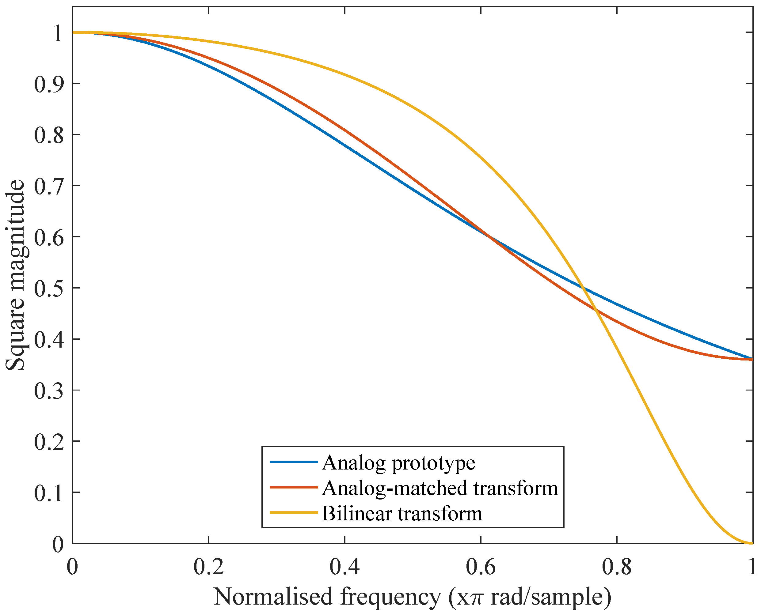
5.2. Digital Equalizer Design Matching Analog Prototypes

Digital filters are frequently derived from analog prototypes, either because analog filter design methods are easily used and understood, or because one is attempting to model analog systems. For example, digital versions of RIAA and NAB equalizers have been proposed [109,110]. The bilinear transform is often used since it offers the desirable properties of preserving order and stability of the analog prototype while mapping the entire continuous-time response onto the unit circle in the z-plane. But it also introduces severe warping as the crossover frequency approaches the Nyquist limit.
The optimization approaches described in Section 5.1 could be used to model an analog equalizer. But they require considerable additional processing and thus are generally performed off-line or at least with latency, or require coefficient tables of sufficient resolution and a suitable interpolation scheme. One could also model and approximate the analog equalizer using differential equations [42], but this is again computationally expensive. Thus these methods are inadequate for controllable and responsive digital equalizer design that matches the analog prototype. Another approach is to use oversampling such that the response over audible frequencies has reduced warping. But this may introduce latency and requires additional anti-aliasing filters.
In this section, we describe a method, first given in [111], for digital equalizer design which anticipates the warping effects and compensates before applying the transform. This give a near optimal match to the analog magnitude response and closed-form expressions for the filter coefficients. Furthermore, the crossover frequency can be specified to be greater than the Nyquist limit.
To illustrate the design process, we show how a lowpass filter matching the analog frequency response may be designed. The first order analog lowpass transfer function with crossover frequency f c is defined as
H LP ( s ) = 1 s / ω c + 1 ,
where ω c = 2 π f c and s = j ω . The square magnitude response | H LP ( ω ) | 2 = 1 / [ 1 + ( ω / ω c ) 2 ] is zero at infinity. But with a standard bilinear transform and prewarping, the digital filter’s zero gain occurs at Nyquist frequency [112] (pp. 535–537). Instead, we start with a first order analog prototype featuring a gain at infinity equal to the desired Nyquist gain. This is achieved using a standard first order analog shelving filter,
H LS ( s ) = g 1 s + Ω s s + Ω s .
We want to set the asymptotic high frequency gain g 1 to be the original magnitude response | H LP | at the Nyquist frequency f s / 2 . The required high frequency gain is then given by
g 1 = | H LP ( s = 2 π f s / 2 ) | = 2 / 4 + f s 2 / f c 2 .
Ordinarily, we would also want to match the gain at the crossover frequency. But when the crossover frequency is close to the Nyquist limit, we observe a steep slope in the digital magnitude response due to the response curve being forced through two close points. So instead, we match the point where the magnitude reaches half Nyquist gain on a Decibel scale. This leads to a matching gain of g m = g 1 and the associated frequency at which | H LP ( ω m ) | = g 1 is ω m = ω c 1 / g 1 1 . The matching frequency specification needs to be prewarped with
Ω m = tan [ ω m / ( 2 f s ) ]
to ensure it will be placed correctly after the bilinear transform with z = e j ω f s . The shelving frequency that provides this match is found by solving | H LS ( Ω m ) | = g m , giving
Ω s = Ω m g 1 .
Applying the bilinear transform leads to the desired lowpass transfer function,
H ( z ) = H LS 1 z 1 1 + z 1 = ( Ω s + g 1 ) + ( Ω s g 1 ) z 1 ( Ω s + 1 ) + ( Ω s 1 ) z 1 .
Figure 13 depicts the square magnitude response for an analog prototype lowpass filter, the digital filter derived from this using the bilinear transform, and the analog-matched digital filter derived using the method herein. Frequency and square magnitude are given on linear scales in order to more easily see the warping with the bilinear transform and the small differences between the analog prototype and the matched-analog digital filter.
Similar approaches for matched-analog digital designs are described in [36] for peaking and notch filters, and in [31] for shelving filters. Or newly proposed analog-to-digital transforms [113] may be used to also give a close match to an analog magnitude response [114]. However, all the standard filters used in digital equalizer design may be matched to analog prototypes by applying the usual transformations in Figure 6 to Equation (55).

5.3. Linear Phase IIR Filters

It is well-known that IIR filters generally are not linear phase. However, several approaches exist for linear phase IIR filter design. Powell and Chau’s real-time linear phase IIR filters [115] used a modification of a well-known time reversal technique. Willson and Orchard described a variation on this approach that yields higher performance (more stopband loss, less passband ripple and/or narrower transition band) [116]. Kurosu et al. described performance issues in Powell and Chau’s original design; a sinusoidal variation in the group delay, and a harmonic distortion with sinusoidal input [117]. To alleviate these issues, they reduce the filter’s overall processing delay by using shorter sections with truncated impulse response [117]. Azizi proposed an efficient arbitrary sample rate converter using zero phase IIR filtering, which later led to a patented signal interpolator [118]. Another approach to linear phase IIR filtering was proposed in [119]. To perform time reversal methods in real time, the signal is divided into blocks of samples. The impulse response of the time-reversed IIR filter must be truncated, but only after it has decayed sufficiently. The cumulative energy of the impulse response can be used for determining an appropriate impulse response length [120].
A basic linear phase IIR method is shown in Figure 14. The input signal passes through a filter H ( z ) , then the order of the samples is reversed, and then this procedure is repeated on the output, i.e, H ( z ) applied, then time reversal. In the time reversal operation, the input signal x [ n ] becomes x [ n ] . The corresponding z-domain transformation can be written as
X ( z ) X ( z 1 ) .
The intermediate transfer functions in Figure 14 can be written as Y 1 ( z ) = H ( z ) X ( z ) , Y 2 ( z ) = H ( z 1 ) X ( z 1 ) , and Y 3 ( z ) = H ( z ) H ( z 1 ) X ( z 1 ) . Thus, the transfer function for the linear phase IIR filter given in Figure 14 is
Y ( z ) = H ( z 1 ) H ( z ) X ( z ) = | H ( z ) | 2 X ( z ) ,
which corresponds to zero phase filtering by the magnitude response of H ( z ) twice.

5.4. Dynamic Equalization

Equalization and dynamics processing are essential signal processing operations in audio engineering. The equalizer is the conventional tool to manipulate the spectral characteristics of the audio signal to achieve frequency balance. In contrast, dynamics processors such as compressors, limiters, gates, expanders and duckers, control the level variation and dynamic envelope of the signal. Among them, the dynamic range compressor [121] is one of the most important tools in mixing, and its use defines much of the sound of contemporary mixes.
Equalization and dynamics processing are often considered to dominate exclusive domains, with equalization controlling amplitude in the spectral domain, and dynamics processing controlling amplitude in the time domain, especially in regard to the input level. Yet those domains are not fully independent. Previous research [122,123] has shown that it is good practice to set dynamic range compressor parameters based on the frequency content in the signal, and many problems in audio production can be addressed by using combinations of filtering and dynamics processing. Thus variants often address specific functionality such as de-essing or hum removal, and as such have limited configurability beyond their applications.
The multiband compressor operates differently and independently on different frequency bands of a signal, offering more precise adjustment of dynamics than a single band compressor. The processing on each frequency band is controlled by its own compression parameters, and output signals of each frequency band are combined as a final step. Unwanted gain changes or artefacts (such as pumping and breathing) are avoided when applying compression on one frequency band. The crossover frequencies are often adjustable.
The dynamic equalizer [4] provides the ballistic control of a dynamic range compressor like threshold, attack and release, to the conventional equalizer allowing time-varying adjustment of equalization curve. In other words, the equalization stage is able to respond dynamically to the input signal level. Many of these dynamic equalizer implementations are used for noise reduction in audio restoration [124], hearing-loss correction [125], and compliance with broadcasting regulations. Other dynamic equalizers employ automatic gain adjustment of a fixed FIR or IIR filter. The modulation can be gated, as in de-hum and de-ess processors [126]. Still other dynamic equalizers allow the filter to be configurable in the band it operates on. The dynamics that most of these systems offer to the engineer are constrained to the point that not all of the details are controllable. Yet the dynamic equalizer is the closest design currently available to the concept of a general frequency and dynamics tool.
Wise proposed a General Dynamic Parametric Equalizer that, in principle, could cover multiband compressors and dynamic equalizers [127]. Conventional multiband compressors compress frequency bands differently through band-pass filters. The general processor utilizes this concept, but replaces these filters with parametric equalizer filters [127]. It offers larger control over the dynamics of specific frequencies or frequency bands in audio signals. It can adjust the frequency, gain, and bandwidth of each filter, with controls common to dynamic range compression controls. The attack and release times determine how fast the dynamic equalization acts towards the defined amount of boost or cut. The characteristic of the processing on each frequency band is controlled by four parameters: gain, threshold, attack, and release. Assuming all parameters are adjustable, this could be configured to a conventional equalizer, dynamic range compressor or multiband compressor. The control characteristics of a multiband compressor and a dynamic equalizer are shown in Figure 15.

6. Sound Reproduction Applications

In this section, we discuss applications in which equalization is used for enhancing audio reproduction, including tone controls, loudspeaker and headphone equalization, room-loudspeaker equalization, loudness equalization, and noise-based equalization.

6.1. Tone Control

Most stereo systems feature tone controls, which provide a quick way to adjust the sound to suit the listener’s taste and compensate for the frequency response of the room. Tone controls are the simplest and possibly most common equalization system. A basic version consists of two knobs, typically labeled "bass" and "treble". These knobs are used to control the gain of low and high frequencies, respectively, through the use of shelving filters (see Section 3). In each case, the maximum gain of the shelf, G, is adjustable. Typical tone controls have an adjustment range of ±12 dB. The crossover frequency is usually fixed. The values for bass and treble vary by manufacturer, but typical crossover frequencies for the bass control might range from 100 Hz to 300 Hz, and the treble control from 3 kHz to 10 kHz. In two-knob tone controls, the midrange frequencies (between bass and treble) are usually left unchanged.
On some units, in addition to control of the bass and treble, there may be a ‘midrange’ or ‘mid’ control. This control is usually implemented as a peaking or notch filter. The knob on the midrange control affects the gain G at center frequency, which generally takes the same range of values as the bass and treble controls, e.g., ±12 dB. The center frequency is generally fixed to be midway between the bass and treble controls, and the bandwidth is chosen so that the midrange control mainly affects the frequencies which are left unadjusted by the bass and treble controls.
Loudness compensation, or loudness control, at low listening levels is another application for equalizing filters in home audio systems [128,129]. The loudness control aims to automatically compensate for the nonlinear behavior of the human hearing system particularly at low frequencies: the equal loudness curves of hearing are compressed at low frequencies with respect to middle and high frequencies. Without the loudness control, as the sound level is turned down, the low-frequency content in music becomes inaudible while middle and higher frequencies are still present [128,129,130,131,132]. Additionally, even when the low-frequency sounds may be heard at soft listening levels, they appear to be more quiet than higher frequencies. A loudness control switch may add one or two shelving or peak filters to the signal path to amplify low frequencies to cancel this nonlinear effect. Alternatively, it is possible to implement a continuous loudness control [128,131,132]. Then the gain and crossover frequency of low-frequency shelving filters are adjusted together with the volume control to modify the rate of level change of low frequencies with volume control. A similar nonlinear compression effect takes place also at very high frequencies, but to a smaller extent. However, it is possible to use high frequency shelving filters for loudness compensation at high frequencies, if desired.
Musical instrument amplifiers use different type of tone control units than other sound systems. They can be specific to the instrument, helping to produce a personal sound quality. For example in a tone stack of a guitar amplifier studied by Yeh and Smith, there are three controls (low, mid, high), but they all control parameters of a third order filter so that their effects overlap [133]. Some electronic keyboard instruments have a built-in tone control circuit, which may have similarly overlapping bands, such as the Clavinet, which has four independent tone equalizing circuits (soft, medium, treble, brilliant) connected in parallel [134].

6.2. Loudspeaker Equalization

One common use of digital equalizers in audio is the flattening of the magnitude response of loudspeakers [78,135,136,137,138,139]. In addition to hi-fi and studio loudspeakers, there are several special categories, such as flat panel speakers [140,141,142,143,144], PA (public address) systems [145,146,147], and micro speakers of mobile devices [148], which benefit from equalization.
The response of the speaker is first measured, usually with the sine-sweep method, in an anechoic room or another special space in which the room effect can be deduced from the impulse response. Unless the loudspeaker under study is a monitor speaker, which is usually aimed directly at the listener, it may be of interest to average the response from a few angles in the frontal sector [149]. The measured magnitude response is usually smoothed using 1/3-octave averaging, which approximately imitates the resolution of human hearing [150]. This implies that very narrow peaks or valleys may not need to be corrected. It is also known that a local peak in the speaker’s magnitude response is more noticeable than a notch [151], and this may be accounted for in the processing of the response.
Loudspeaker response equalization always requires a target response against which the measured and smoothed speaker response is compared [108,138]. The target response generally cannot be constant across all frequencies. Loudspeakers are inherently highpass systems, having a low-frequency crossover point below which they cannot produce sound effectively. An attempt to boost the response beyond this point leads to increased distortion and may even destroy the speaker, if its cone is forced to exceed the maximum deviation. One easy way to obtain a target curve at low frequencies is to use the magnitude response of a Butterworth highpass filter, which is smooth and does not overshoot. A reasonable crossover frequency, in the range 30 to 100 Hz, should be selected, which is near the natural low-frequency point of the speaker. A second order Butterworth highpass filter having an approximately 12-dB per octave slope is suitable for producing the target response for regular dynamic loudspeakers, while a fourth order highpass filter with a 24-dB/oct. slope should be used for vented (bass reflex) speakers. The ratio of the measured and target responses, or the difference between the dB magnitude responses, yields the necessary correction as a function of frequency. Matched filter design methods discussed in Section 5.1 and the high-precision graphic equalizer of Section 4.3 are good candidate methods for designing the equalizer.
Usually loudspeakers divide the audio band for two or three speaker elements, because a single element cannot reproduce the whole audio band with good quality [78]. The input signal is delivered to each element via a crossover network, which implements a selective filter (lowpass, bandpass, or highpass) for each element. The most common crossover filter design is the Linkwitz-Riley network [78,152]. Each element can be equalized separately after the crossover filtering [78,136,149]. One possibility is to combine the equalizers and the crossover filters, as suggested by Ramos and López [153].
Various equalization filters and design methods have been proposed for loudspeaker equalization, including automatic adjustment of parametric equalizers [154,155]. Karjalainen et al. first suggested the use of warped FIR and IIR filters for loudspeaker equalization to ease the approximation at low frequencies [138,156]. Warped filters then became a popular method for equalizing loudspeakers [138,157,158,159]. Ramos et al. have proposed to use a cascade connection of a regular and a warped FIR filter [160]. The balanced model truncation method is applied in [161].
In addition to magnitude-only equalization, also phase equalization of loudspeakers is sometimes considered, especially at low frequencies [138,162]. This can be combined with the magnitude response equalization, which leads to complex frequency response equalization, or it can be realized separately using a delay equalizer, which is usually based on allpass filter design. Herzog and Hilsamer have proposed to simulate the group delay at low frequencies using an allpass filter and then to implement the phase equalization by filtering the input signal in short blocks backwards in time [162], similar to the linear phase IIR filter design described in Section 5.3. This solution produces an inevitable processing delay. Alternatively, it is possible to design a high order allpass filter, for example using the method proposed by Abel and Smith [163].

6.3. Room Equalization

One common use of graphic equalization is to “tune” a room, adjusting the equalizer to roughly compensate for room resonances. The goal is to achieve a desired magnitude response, flattening out extremes, reducing coloration in the sound and achieving greater sonic consistency among listening spaces. Graphic equalization is more commonly found in live performance and recording studios than in most home stereo systems. However, graphic equalizers are occasionally found in consumer stereo systems and even in digital music player software, where they can be used as a more flexible form of tone control for refining the sound according to one’s taste. In addition to studios, performance venues, and living rooms, equalization of a listening space is highly relevant in car cabins [49,164,165,166,167,168].
A traditional way to equalize a loudspeaker in a room is to consider loudspeaker equalization and room equalization separately [169]. First the anechoic response of the loudspeaker is equalized using an equalizer, and then the equalized speaker is measured in a room, and a second equalizer is designed. In more recent approaches, a measured anechoic speaker response is no longer required. It is now known that acoustic impulse responses of typical listening spaces are short at high and middle frequencies, but can be very long at low frequencies. For this reason, one idea is to use a gated (truncated) version of the loudspeaker impulse response in a room to model the first equalizer [108,170]. After that another equalizer may be designed to correct the response at low frequencies. Bank and Ramos have proposed techniques for automatically selecting the poles of parallel IIR filters, which has the same structure as the parallel graphic equalizer in Section 4.3, to equalize the loudspeaker-room response [171].
There are two radically different scenarios in room equalization: the single-point and multiple-point cases [164]. In the single-point case, the loudspeaker-room response is equalized for a ‘sweet spot,’ which may be the main listening position or a microphone location. However, this approach usually decreases the sound quality at other locations in the room, and thus is rarely a good solution [164,172,173]. In multi-point room equalization, the response is measured at two or more listening positions, and the equalizer is designed to improve the response at all of them. Naturally, this may not be achieved fully at any location, so the equalizer design becomes an optimization problem [164]. One useful idea is to suppress the room modes appearing at all measured locations, which are called common acoustical poles [174,175]. Other approaches to multi-point room equalization include spatial averaging [176] and effort variation [177].
Related problems are the shortening of the room impulse response and reduction of the room reverberation, which is called dereverberation [173,178]. It is known that when the reproduced sound in a room becomes boomy, it may not be enough to suppress the level of sound at that frequency with an equalizer, since that mode will still remain ringing, although less loudly. A special method for shortening low-frequency room modes is called modal equalization [178,179]. It involves estimating, canceling, and replacing single ringy room modes, which appear at frequencies below about 200 Hz. The cancellation filter is a digital notch filter while a resonator is used for replacing it with a more quickly decaying response [179]. Karjalainen et al. have suggested an iterative method to find the longest decaying modes at low frequencies using high order pole-zero modeling on a downsampled band, which is called frequency-zooming ARMA modeling [180]. Fazenda et al. have studied the audibility of low-frequency modes, which is important to know when designing a modal equalizer [181].
In acoustic impulse response shortening, the aim is to modify the decay rate of room reverberation, but not to cancel it fully [182,183]. This can improve the sound quality and intelligibility. Impulse response reshaping can be combined with crosstalk cancellation in spatial sound reproduction systems in which it is necessary to control the sounds reaching the ears of a listener [184]. Dereverberation is particularly important for speech, because room reverberation reduces speech intelligibility in telephone and teleconferencing systems and complicates automatic speech recognition [185,186].

6.4. Headphone Equalization

Equalization of headphones is largely based on the same general principle as loudspeaker equalization with a few differences [187,188]: measure the impulse response of the system, compute the corresponding smoothed magnitude response, compare it against a target response, design an equalizer to minimize the difference between the measured and target responses, and implement the equalizing filter, which should process the input signal of the system. A sine sweep is commonly used for measuring the impulse response of headphones. The main differences between loudspeaker and headphone equalization are in the measurement of the impulse response and in the shape of the target response.
In the case of headphones, there are only two impulse responses to be measured per headphone, those from the left and right earpiece. However, variations in these responses can easily appear since the fit of the headphones can have a major effect on their frequency response. If the headphones are not tightly fitted, the low-frequency response can suffer considerable attenuation. This is especially prominent in in-ear headphones, in which the earpiece is similar to an earplug [189]. The headphone response is easiest to measure using a dummy head. Miniature microphones inside the ear canal must be mounted when headphones are measured while they are worn by a user. Bolaños and Pulkki have proposed a method to measure the headphone response of the user at the ear canal entrance and map it to the eardrum [190]. This method requires measuring both the acoustic velocity and the pressure.
There are different options for the headphone target response, which are usually not flat, as shown in Figure 16. The free field response corresponds to listening to a sound source with a flat magnitude response located in front of the listener in an anechoic room. The free field response is seen to contain resonances, the highest of which appears at approximately 3 kHz and compensates for the open ear canal resonance, which is suppressed when the headphones cover the entrance to the ear. Additionally, the free-field response is attenuated around 8 kHz to cancel a closed ear canal resonance, which appears when wearing headphones. The diffuse-field response, also shown in Figure 16, can be measured with a dummy head in an echo chamber. It corresponds to listening to an omnidirectional loudspeaker located far away from the listener, so that in the echo chamber the sound appears to come from all directions, i.e., the sound field is diffuse.
Olive et al. [191] have conducted extensive studies trying to find out the preferred target response for headphone listening. The blue curve in Figure 16 is their new target response, which corresponds to listening to a high-quality speaker in a room. They suggest that this curve should be used as the prototype curve for good headphones for music listening [191]. It may be noticed that this target curve has a large boost at approximately 3 kHz and also a shelf-like boost of about 5 dB at frequencies below 100 Hz. High frequencies are attenuated more than in free or diffuse-field responses.
The magnitude response of headphones often contains notches at high frequencies, which also change their location when the headphones move in the head of the listener. For this reason, it is typical not to attempt to equalize headphones at frequencies higher than about 10 kHz. To avoid the spectral notches from causing large gain peaks or ringing in the equalization filter response, regularization techniques can be used [192,193].
In addition to correcting the headphone response to be closer to a chosen target response, it is possible to design an equalizer to imitate the response of another pair of headphones. This idea was first proposed by Briolle and Voinier, who simulated various headphones by convolving the input signal with the headphone impulse response [194]. Olive et al. [195] have compared headphone responses in a similar fashion while Rämö and Välimäki [192] also included an equalizer modeling the acoustic isolation response of the headphones, so that the ambient noise could be included in the simulation.
Another headphone application based on equalization filters is the modeling of head-related transfer functions (HRTF), which leads way to three-dimensional sound reproduction [196,197]. Various digital filter design methods, such as balanced model truncation [198] and cascaded peak/notch filters [51,199], have been used for modeling HRTF responses [200]. Simplification of HRTF filters has been used for demonstrating which spectral details are required for hearing directions correctly [201]. Hiekkanen et al. have developed a method to compare loudspeakers using headphones with equalization filters, which are based on HRTF responses [202].
In augmented reality audio, a headset having microphones near the user’s ears is used for combining reproduced and ambient sounds [203,204,205,206]. The ambient sounds captured by the microphones must be equalized to enhance their naturalness [203,205,207]. Also the isolation of the headphones must be accounted for, since the leaked and reproduced ambient sound both reach the user’s ear [208,209]. The equalization of the microphone signal requires shelving and peak/notch filters [188,208]. A related application is a real-time audio equalizer, which processes the external microphone sounds to be played instantly through the headphones, for example to enhance the perceived sound in a concert [210].

6.5. Equalization to Combat Ambient Noise

When music listening takes place in a noisy environment, such as in a speeding car or bus, the ambient noise can considerably disturb the hearing experience [211]. A traditional solution to this in car radios and audio systems has been the automatic gain control, which adjusts the volume according to car speed or background noise level inside the car cabin [212,213,214]. Additionally, dynamic range compression [121] may be used to reduce loudness changes, since the softest passages of music easily become inaudible in noise [212,215]. However, since the ambient noise hardly ever has a flat spectrum but usually contains more energy at low frequencies, like pink noise, simply increasing the gain is not the best way to combat this: the gain should usually be increased more at low frequencies than at high frequencies.
It is well understood that background noise disturbs the listening experience through the auditory masking phenomenon. It causes the hearing threshold to increase mostly at those frequencies where the noise signal has energy. Additionally, the masking phenomenon spreads to other frequencies, so that higher frequencies than the noise component are more affected and lower frequencies less. Rämö et al. have convincingly simulated this phenomenon for headphone listening in noise [216]: a graphic equalizer having a resolution of the auditory Bark bands controlled by an auditory model imitates the increase of the hearing threshold. This simulation of noise-based masking allows one to listen to music samples without both the noise and those components that get masked by the noise.
Miller and Barish have described a Dynamic Sound Optimization system for cars, which analyzes the ambient noise from signals captured by microphones [217]. Figure 17(a) shows a single-channel version of this system. Adaptive filtering is first used to separate the background noise from the microphone signal by using the music signal as the reference. This is the same principle as in adaptive echo canceling (AEC), which is used for suppressing the near-end signal in telephone and teleconferencing systems [218]. Based on the analysis of the extracted noise signal, a low-frequency shelving filter, a variable equalizer, and a dynamic range compressor are controlled to effectively cancel the auditory masking experienced by the passengers. When more loudspeakers are used, their signals can be canceled from the microphone signal one after the other [217]. Tzur and Goldin [219], Kim and Cho [50], and Christoph [214] have proposed a noise-based equalizer using an FFT filterbank. The music or speech signal to be played in a noisy environment, such as in a car, is processed with the filterbank so that the gain of each Bark-band depends on estimated masking caused by the ambient noise signal.
Headphones have become highly popular in recent years, because they are now the common way of listening to music and other sounds from mobile phones and tablet computers. The mobile use of headphones mostly happens in noisy environments, such as in cities with heavy traffic and on buses, trains, and airplanes [215]. Additionally, headphones are used in noisy work places for personal audio and for sound shading, which refers to pleasant masking noise to hide for example conversations. In all these use cases, the background noise disturbs the listening experience, and so it becomes important to select headphones with good noise attenuation, possibly combined with active noise control [192]. Still, some ambient noise may leak to the user’s ear, masking the music signal at some frequencies.
Rämö et al. [220] and Välimäki et al. [206] have described a noise-based equalization system for headphone listening, which is sketched in Figure 17(b). It captures the ambient noise using an external microphone, such as the one in the cord of a hands-free headset, typically used for the user’s own voice. This ambient noise signal is processed with a filter, which models the estimated isolation of noise through the headphone to the ear. By using the processed ambient noise signal as the masker and the music signal played through the headphones as the desired signal, it is possible with an auditory model to estimate the masking as a function of frequency. This information is used for controlling an equalizer, which aims to cancel the masking phenomenon. A graphic equalizer with Bark-band division was used in which the filter bandwidth is constant 100 Hz for the lowest five band and approximately one-third octave for the other bands [220].

7. Audio Content Creation

Equalization and its use in the music production process has become well-established, with standardized designs for graphic and parametric equalizers, and well-established operations to achieve desired tasks [221]. However, in recent years there has been an emergence of adaptive, intelligent or autonomous audio equalizers, which provide novel approaches to their design and use. This section gives an overview of these new directions in equalization for content creation.

7.1. Adaptive and Intuitive Interfaces

Here, we provide an overview of the state of the art concerning interfaces for equalization, with an emphasis on perceptual adaptive and intuitive controls. Various approaches for learning a listener’s preferences for an equalization curve with a small number of frequency bands have been applied to research in the setting of hearing aids [222,223] and cochlear implants [224], and the modified simplex procedure [225,226] is now an established approach for selecting hearing aid frequency responses. However, many recent innovations have emerged in the field of music production.
In [227], Dewey and Wakefield evaluated various novel equalizer interface designs that incorporated spectral information in addition to or as a replacement for equalization curves and parametric controls. Their subjective evaluation suggested that such designs may be more efficient and preferred over traditional interfaces for many equalization tasks. Loviscach presented an interface for a five-band parametric equalizer where the user simply freehand draws the desired magnitude response and an evolutionary optimization strategy (chosen for real-time interaction) finds the closest match [228]. Informal testing suggested that this interface reduced the set-up time for a parametric equalizer compared to more traditional interfaces. Building on this, Heise et al. proposed a procedure to achieve equalization and other effects using a black-box genetic optimization strategy [229]: Users are confronted with a series of comparisons of two differently processed sound examples. Parameter settings are optimized by learning from the users’ choices. Though these interfaces are novel and easy to use by the nonexpert, they make no use of semantics or descriptors.
Considerable research has aimed at the development of technologies that let musicians or sound engineers perform equalization using perceptually relevant or intuitive terms, e.g. brightness, warmth, or presence. Reed presented an assistive sound equalization expert system [230]. Inductive learning based on nearest neighbor pattern recognition was used to acquire expert skills. These were then applied to adjust the timbral qualities of sound in a context-dependent fashion. They emphasized that the system must be context-dependent, that is, the equalization depends on the input signal system and hence operates as an adaptive audio effect. In [231], a self-organizing map was trained to represent common equalizer settings in a two-dimensional (2-D) space organized by similarity. The space was hand-labelled with descriptors that the researchers considered to be intuitive. However, informal subjective evaluation suggested that users would like to choose their own descriptors.
The work of Bryan Pardo and his collaborators has focused on new, intelligent and adaptive interfaces for equalization tasks. They address the challenge that complex interfaces for equalizers can prevent novices from achieving their desired modifications. Sabin and Pardo described and evaluated an algorithm to rapidly learn a listener’s desired equalization curve [232,233,234,235]. Listeners were asked to indicate how well an equalized sound could be described by a perceptual term. After rating, weightings for each frequency band were found by correlating the gain at each frequency band with listener responses, thus providing a mapping from the descriptors to audio processing parameters. Listeners reported that the resultant sounds captured their intended meanings of descriptors, and machine ratings generated by computing the similarity of a given curve to the weighting function were highly correlated to listener responses. This allows automated construction of a simple and intuitive audio equalizer interface. In [236], active and transfer learning techniques were applied to exploit knowledge from prior concepts taught to the system from prior users, greatly enhancing the performance of the equalization learning algorithm.
The early work on intelligent equalization based on intuitive descriptors was hampered by a limited set of descriptors with a limited set of training data to map those descriptors to equalizer settings. Cartwright and Pardo addressed this with SocialEQ, a web-based crowdsourcing application aimed at learning the vocabulary of audio equalization descriptors [237]. To date, 633 participants have participated in a total of 1102 training sessions (one session per learned word), of which 731 sessions were deemed reliable in the sense that users were self-consistent in their answers (Personal communication with B. Pardo, 2015). This resulted in 324 distinct terms, and data on these terms is made available for download.
Building on the mappings from descriptors to equalization curves, Sabin and Pardo [233] described a simple equalizer where the entire set of curves were represented in a 2-D space (similar to [231]), thus assigning spatial locations to each descriptor. Equalization is performed by the user dragging a single dot around the interface, which simultaneously manipulates 40 bands of a graphic equalizer. This approach was extended to multitrack equalization in [238], which provided an interface that, by varying simple graphic equalizers applied to each track in a multitrack, allowed the user to intuitively explore a diverse set of mixes.
The concepts of perceptual control, learned from crowdsourcing, intuitive interface design and mapping of a high dimensional parameter space to a lower dimensional representation were all employed in [239,240]. This approach scaled equalizer parameters to spectral features of the input signal, then mapped the equalizer’s 13 controls to a 2-D space. The system was trained with a large set of parameter space data representing warmth and brightness, measured across a range of musical instrument samples, allowing users to perform equalization using a perceptually and semantically relevant, simple interface.

7.2. Autonomous and Intelligent Systems for Equalization

As a recent example application of targeted equalization (see Section 5.1), Ma et al. [241] described an intelligent equalization tool that, in real-time, equalized an incoming audio stream towards a target frequency spectrum. The target spectrum was derived from analysis of 50 years of commercially successful recordings [242]. The target equalization curve is thus determined by the difference in spectrum between an incoming signal and this target spectrum. A hysteresis gate is first applied on the incoming signal, to ensure that only active content (i.e., not silence or low level noise) is used to estimate the input signal spectrum. Since the input signal to be equalized is continually changing, the desired magnitude response of the target filter is also changing (though the target output spectrum remains the same). Thus, smoothing was applied from frame to frame on the desired magnitude response D ( ω ) and on the applied filter H ( ω ) . Targeting was achieved using the Yule-Walker method, and testing showed that Yule-Walker offered superior performance to the method proposed by Lee [98]. Figure 18 depicts a block diagram of this system.
Perez Gonzalez and Reiss described a method for automatically equalizing a multitrack mixture [243]. The method aimed to achieve equal average perceptual loudness on all frequencies amongst all tracks within a multitrack audio stream. Accumulative spectral decomposition techniques were used together with cross-adaptive audio effects to apply graphic equalizer settings to each track. Analysis demonstrated that this automatic equalization method was able to achieve a well-balanced and equalized final mix.
An alternative approach to autonomous multitrack equalization was provided by Hafezi and Reiss [244]. They created a multitrack intelligent equalizer that used a measure of auditory masking and rules based on best practices from the literature to apply, in real-time, different multiband equalization curves to each track. The method is intended as a component of an automatic mixing system that applies equalization as it might be applied manually as part of the mixing process. Results of objective and subjective evaluation were mixed and showed room for improvement, but they indicated that masking was reduced and the resultant mixes were preferred over amateur, manual mixes.
Finally, Barchiesi and Reiss showed how to reverse engineer the equalization settings applied to each track in a multitrack mix [245]. That is, given a multitrack recording and the mixed output track, the settings of all time-varying equalizers applied to each track can be derived. Assuming that mixing involves the processing of each input track by a linear time-invariant (LTI) system (slowly time varying processing may be valid if a frame-by-frame approach is applied), then a least squares approach may be used to find the impulse response applied to each track. This impulse response represents all the LTI effects that might be applied during the mixing process, including gains, delays, stereo panners, and equalization filters. Equalization is distinguished from delays, gains and panning by assuming that equalization introduces the minimum possible delay, that the equalization does not affect the signal level, and that level differences between channels are due to stereo panning. If the multitrack recording was mixed using FIR filters, then the estimation order can be increased until an almost exact solution is obtained. If IIR filters were used, then either one estimates the IIR filter best approximating the finite impulse response, or nonlinear or iterative least squares approaches are used to derive the filter coefficients directly. Reported results showed the effectiveness of their approach with 4, 6 and 8 track multitracks, when both IIR and (up to 128th order) FIR filters were applied, and when there was no knowledge of the characteristics of the (third party, commercial) filters that were applied.

8. Conclusions

In this review paper, we described audio equalization in terms of its historical perspective, the established designs and approaches, and the frontier research directions and emerging challenges. Though low order parametric and graphic equalizers are well-established, variations and extensions of these designs, such as high order parametric equalizers or convolution-based graphic equalizers, offer almost limitless ability to shape the spectral content of a signal. These design choices allow the user or designer to favour precise control, low computational cost and/or minimal latency. Moving away from graphic and parametric equalizers, other approaches allow for the design of equalization filters that combine the most appealing features of IIR and FIR filters, or provide the means to match an arbitrary magnitude (or magnitude and phase) response. A summary of approaches to equalization and their relevant features and applications is given in Table 3.
The applications of these designs are vast, with equalization being relevant to any situation where it may be of benefit to shape a spectrum. Of note, loudspeaker, room and headphone equalization are common, but equalizers have uses throughout the music recording, production and playback chain. A particularly relevant application in today’s busy world is the noise-based equalization, which can enhance the audibility of music in high ambient noise. Finally, Section 7 considered new and emerging approaches to equalization. It focused on more relevant and intuitive interfaces, often based on machine learning, and on autonomous and intelligent audio equalization systems that attempt to automate aspects of their use. This area is still in its infancy, and might see great advances with improved knowledge of the semantics and perceptual aspects of equalization.

Acknowledgments

We would like to thank our colleagues Riitta Väänänen, Jonathan S. Abel, Fabián Esqueda, Ville Pulkki, German Ramos, Jussi Rämö, Julius O. Smith, Miikka Tikander, and Sampo Vesa for helpful comments and discussions on audio equalizers. Special thanks go to Juho Liski for his help on producing the headphone target response figure.

Author Contributions

The authors contributed equally to this work.

Conflicts of Interest

The authors declare no conflict of interest.

Appendix

The source code for the methods discussed in this paper and for many of the figures are available online at https://code.soundsoftware.ac.uk/projects/allaboutaudioeq. It includes;
  • Matlab code demonstrating a parametric equalizer comprised of a first order low shelving filter, second order peaking/notch filter and first order high shelving filter, see Section 3, especially Section 3.1 and Section 3.3;
  • Matlab code for second order low and high shelving filter, see Section 3.2.
  • Matlab code for generating a wide variety of high order filter designs of arbitrary order and for differing definitions of the gain at crossover frequencies, see Section 3.4;
  • Matlab code for cascade and parallel graphic equalizer design, see Section 4;
  • Matlab code for a lowpass filter matching the analog frequency response, see Section 5.2;
  • Matlab code for illustrating dynamic equalization and multiband dynamic range compression, see Section 5.4;
  • A Powerpoint file containing original versions of many of the figures; and
  • Any additions or errata since initial publication.

References

  1. Bohn, D.A. Operator adjustable equalizers: An overview. In Proceedings of the Audio Engineering Society 6th International Conference on Sound Reinforcement, Nashville, Tennessee, 5–8 May 1988; pp. 369–381.
  2. Orfanidis, S.J. IIR digital filter design (Chapter 11). In Introduction to Signal Processing; Prentice Hall: Englewood Cliffs, NJ, USA, 1996; pp. 573–643. [Google Scholar]
  3. Zölzer, U. Equalizers (Chapter 5). In Digital Audio Signal Processing, 2nd ed.; Wiley: Chichester, UK, 2008; pp. 115–190. [Google Scholar]
  4. Reiss, J.D.; McPherson, A. Filter effects (Chapter 4). In Audio Effects: Theory, Implementation and Application; CRC Press: Boca Raton, FL, USA, 2015; pp. 89–124. [Google Scholar]
  5. Lundheim, L. On Shannon and Shannon’s formula. Telektronikk 2002, 98, 20–29. [Google Scholar]
  6. Campbell, G.A. Physical theory of the electric wave-filter. Bell Syst. Tech. J. 1922, 1, 1–32. [Google Scholar] [CrossRef]
  7. Zobel, O.J. Theory and design of uniform and composite electric wave-filters. Bell Syst. Tech. J. 1923, 2, 1–46. [Google Scholar] [CrossRef]
  8. Bauer, B. A century of microphones. Proc. IRE 1962, 50, 719–729. [Google Scholar] [CrossRef]
  9. Williamson, D.T.N. Design of tone controls and auxiliary gramophone circuits. Wireless World 1949, 55, 20–29. [Google Scholar]
  10. Baxandall, P.J. Negative-feedback tone control. Wireless World 1952, 58, 402–405. [Google Scholar]
  11. Stanton, W.O. Magnetic pickups and proper playback equalization. J. Audio. Eng. Soc. 1955, 3, 202–205. [Google Scholar]
  12. Hoff, P. Tape (NAB) equalization. In Consumer Electronics for Engineers; Cambridge University Press: Cambridge, UK, 2008; pp. 131–135. [Google Scholar]
  13. Rudmose, W. Equalization of sound systems. Noise Control 1958, 24, 82–85. [Google Scholar] [CrossRef]
  14. Boner, C.P.; Boner, C.R. Minimizing feedback in sound systems and room-ring modes with passive networks. J. Acoust. Soc. Am. 1965, 37, 131–135. [Google Scholar] [CrossRef]
  15. Boner, C.P.; Boner, C.R. Behavior of sound system response immediately below feedback. J. Audio. Eng. Soc. 1966, 14, 200–203. [Google Scholar]
  16. Conner, W.K. Theoretical and practical considerations in the equalization of sound systems. J. Audio Eng. Soc. 1967, 15, 194–198. [Google Scholar]
  17. Flickinger, D. Amplifier System Utilizing Regenerative and Degenerative Feedback to Shape the Frequency Response. U.S. Patent #3,752,928, 14 August 1973. [Google Scholar]
  18. Massenburg, G. Parametric equalization. In Proceedings of the 42nd Convention of the Audio Engineering Society, Los Angeles, CA, USA, 2–5 May 1972.
  19. McNally, G.W. Microprocessor mixing and processing of digital audio signals. J. Audio Eng. Soc. 1979, 27, 793–803. [Google Scholar]
  20. Guarino, C.R. Audio equalization using digital signal processing. In Proceedings of the 63rd Convention of the Audio Engineering Society, Los Angeles, CA, USA, 15–18 May 1979.
  21. Hirata, Y. Digitalization of conventional analog filters for recording use. J. Audio Eng. Soc. 1981, 29, 333–337. [Google Scholar]
  22. Berkovitz, R. Digital equalization of audio signals. In Proceedings of the Audio Engineering Society 1st International Conference on Digital Audio, Rye, NY, USA, 3–6 June 1982.
  23. White, S.A. Design of a digital biquadratic peaking or notch filter for digital audio equalization. J. Audio Eng. Soc. 1986, 34, 479–483. [Google Scholar]
  24. Regalia, P.; Mitra, S. Tunable digital frequency response equalization filters. IEEE Trans. Acoust. Speech Signal Process. 1987, 35, 118–120. [Google Scholar] [CrossRef]
  25. Brandt, M.; Bitzer, J. Hum removal filters: Overview and analysis. In Proceedings of the 132nd Convention of the Audio Engineering Society, Budapest, Hungary, 26–29 April 2012.
  26. Van Waterschoot, T.; Moonen, M. Fifty years of acoustic feedback control: State of the art and future challenges. Proc. IEEE 2011, 99, 288–327. [Google Scholar] [CrossRef]
  27. Harris, f.; Brooking, E. A versatile parametric filter using an imbedded all-pass sub-filter to independently adjust bandwidth, center frequency, and boost or cut. In Proceedings of the Asilomar Conference on Signals, Systems and Computers, Pacific Grove, CA, USA, 26–28 October 1992; pp. 269–273.
  28. Moorer, J.A. The manifold joys of conformal mapping: Applications to digital filtering in the studio. J. Audio Eng. Soc. 1983, 31, 826–841. [Google Scholar]
  29. Constantinides, A. Spectral transformations for digital filters. Proc. IEE 1970, 117, 1585–1590. [Google Scholar] [CrossRef]
  30. Fontana, F.; Karjalainen, M. A digital bandpass/bandstop complementary equalization filter with independent tuning characteristics. IEEE Signal Process. Lett. 2003, 10, 119–122. [Google Scholar] [CrossRef]
  31. Berners, D.P.; Abel, J.S. Discrete-time shelf filter design for analog modeling. In Proceedings of the 115th Convention of the Audio Engineering Society, New York, NY, USA, 10–13 October 2003.
  32. Keiler, F.; Zölzer, U. Parametric second- and fourth-order shelving filters for audio applications. In Proceedings of the IEEE Workshop on Multimedia Signal Processing, Siena, Italy, 29 September–1 October 2004; pp. 231–234.
  33. Christensen, K.B. A generalization of the biquadratic parametric equalizer. In Proceedings of the 115th Convention of the Audio Engineering Society, New York, NY, USA, 10–13 October 2003.
  34. Jot, J.M. Proportional parametric equalizers—Application to digital reverberation and environmental audio processing. In Proceedings of the 139th Convention of the Audio Engineering Society, New York, NY, USA, 29 September–1 October 2015.
  35. Clark, R.J.; Ifeachor, E.C.; Rogers, G.M.; Van Eetvelt, P.W. Techniques for generating digital equalizer coefficients. J. Audio Eng. Soc. 2000, 48, 281–298. [Google Scholar]
  36. Orfanidis, S.J. Digital parametric equalizer design with prescribed Nyquist-frequency gain. J. Audio Eng. Soc. 1997, 45, 444–455. [Google Scholar]
  37. Bristow-Johnson, R. The equivalence of various methods of computing biquad coefficients for audio parametric equalizers. In Proceedings of the 97th Convention of the Audio Engineering Society, San Francisco, CA, USA, 10–13 November 1994.
  38. Reiss, J.D. Design of audio parametric equalizer filters directly in the digital domain. IEEE Trans. Audio Speech Lang. Process. 2011, 19, 1843–1848. [Google Scholar] [CrossRef]
  39. Orfanidis, S.J. High-order digital parametric equalizer design. J. Audio Eng. Soc. 2005, 53, 1026–1046. [Google Scholar]
  40. Holters, M.; Zölzer, U. Parametric higher-order shelving filters. In Proceedings of the European Signal Process. Conference (EUSIPCO), Florence, Italy, 4–8 September 2006; pp. 1–4.
  41. Fernandez-Vazquez, A.; Rosas-Romero, R.; Rodriguez-Asomoza, J. A new method for designing flat shelving and peaking filters based on allpass filters. In Proceedings of the International Conference on Electronics, Communications and Computers (CONIELECOMP-07), Cholula, Puebla, Mexico, 26–28 February 2007.
  42. Särkkä, S.; Huovilainen, A. Accurate discretization of analog audio filters with application to parametric equalizer design. IEEE Trans. Audio Speech Lang. Process. 2011, 19, 2486–2493. [Google Scholar] [CrossRef]
  43. Lim, Y.C. Linear-phase digital audio tone control. J. Audio Eng. Soc. 1987, 35, 38–40. [Google Scholar]
  44. Lian, Y.; Lim, Y.C. Linear-phase digital audio tone control using multiplication-free FIR filter. J. Audio Eng. Soc. 1993, 41, 791–794. [Google Scholar]
  45. Yang, R.H. Linear-phase digital audio tone control using dual RRS structures. Electron. Lett. 1989, 25, 360–362. [Google Scholar] [CrossRef]
  46. Vieira, J.M.N.; Ferreira, A.J.S. Digital tone control. In Proceedings of the 98th Convention of the Audio Engineering Society, Paris, France, 25–28 February 1995.
  47. Greiner, R.A.; Schoessow, M. Design aspects of graphic equalizers. J. Audio Eng. Soc. 1983, 31, 394–407. [Google Scholar]
  48. Takahashi, S.; Kameda, H.; Tanaka, Y.; Miyazaki, H.; Chikashige, T.; Furukawa, M. Graphic equalizer with microprocessor. J. Audio Eng. Soc. 1983, 31, 25–28. [Google Scholar]
  49. Kontro, J.; Koski, A.; Sjöberg, J.; Väänänen, M. Digital car audio system. IEEE Trans. Consum. Electron. 1993, 35, 514–521. [Google Scholar] [CrossRef]
  50. Kim, H.G.; Cho, J.M. Car audio equalizer system using music classification and loudness compensation. In Proceedings of the International Conference on ICT Convergence (ICTC), Seoul, Korea, 28–30 September 2011; pp. 553–558.
  51. Abel, J.S.; Berners, D.P. Filter design using second-order peaking and shelving sections. In Proceedings of the International Computer Music Conference, Coral Gables, FL, USA, 1–6 November 2004.
  52. Holters, M.; Zölzer, U. Graphic equalizer design using higher-order recursive filters. In Proceedings of the International Conference on Digital Audio Effects (DAFX), Montreal, QC, Canada, 18–20 September 2006; pp. 37–40.
  53. Rämö, J.; Välimäki, V. Optimizing a high-order graphic equalizer for audio processing. IEEE Signal Process. Lett. 2014, 21, 301–305. [Google Scholar] [CrossRef]
  54. Motorola Inc. Digital stereo 10-band graphic equalizer using the DSP56001. Appl. Note 1988, APR2/D. [Google Scholar]
  55. Tassart, S. Graphical equalization using interpolated filter banks. J. Audio Eng. Soc. 2013, 61, 263–279. [Google Scholar]
  56. Rämö, J.; Välimäki, V.; Bank, B. High-precision parallel graphic equalizer. IEEE/ACM Trans. Audio Speech Lang. Process. 2014, 22, 1894–1904. [Google Scholar] [CrossRef]
  57. Adams, R.W. An automatic equalizer/analyzer. In Proceedings of the 67th Convention of the Audio Engineering Society, New York, NY, USA, 31 October–3 November 1980.
  58. Erne, M.; Heidelberger, C. Design of a DSP-based 27 band digital equalizer. In Proceedings of the 90th Convention of the Audio Engineering Society, Paris, France, 19–22 February 1991.
  59. Azizi, S.A. A new concept of interference compensation for parametric and graphic equalizer banks. In Proceedings of the 111th Convention of the Audio Engineering Society, New York, NY, USA, 30 November–3 December 2001.
  60. Miller, R. Equalization methods with true response using discrete filters. In Proceedings of the 116th Convention of the Audio Engineering Society, Berlin, Germany, 8–11 May 2004.
  61. ISO. ISO 266, Acoustics—Preferred frequencies for measurements. 1975. [Google Scholar]
  62. Bohn, D.A. Constant-Q graphic equalizers. J. Audio Eng. Soc. 1986, 34, 611–626. [Google Scholar]
  63. Oliver, R.J.; Jot, J.M. Efficient multi-band digital audio graphic equalizer with accurate frequency response control. In Proceedings of the 139th Convention of the Audio Engineering Society, New York, NY, USA, 29 September–1 October 2015.
  64. Lee, Y.; Kim, R.; Cho, G.; Choi, S.J. An adjusted-Q digital graphic equalizer employing opposite filters. In Lect. Notes Comput. Sci.; Springer-Verlag: London, UK, 2005; Volume 3768, pp. 981–992. [Google Scholar]
  65. McGrath, D.; Baird, J.; Jackson, B. Raised cosine equalization utilizing log scale filter synthesis. In Proceedings of the 117th Convention of the Audio Engineering Society, San Francisco, CA, USA, 28–31 October 2004.
  66. Chen, Z.; Lin, Y.; Geng, G.; Yin, J. Optimal design of digital audio parametric equalizer. J. Inform. Comput. Sci. 2014, 11, 57–66. [Google Scholar] [CrossRef]
  67. Belloch, J.A.; Bank, B.; Savioja, L.; Gonzalez, A.; Välimäki, V. Multi-channel IIR filtering of audio signals using a GPU. In Proceedings of the IEEE International Conference Acoustics, Speech and Signal Processing (ICASSP), Florence, Italy, 4–9 May 2014; pp. 6692–6696.
  68. Bank, B. Perceptually motivated audio equalization using fixed-pole parallel second-order filters. IEEE Signal Process. Lett. 2008, 15, 477–480. [Google Scholar] [CrossRef]
  69. Bank, B. Audio equalization with fixed-pole parallel filters: An efficient alternative to complex smoothing. J. Audio Eng. Soc. 2013, 61, 39–49. [Google Scholar]
  70. Belloch, J.A.; Välimäki, V. Efficient target response interpolation for a graphic equalizer. In Proceedings of the IEEE International Conference Acoustics, Speech and Signal Processing (ICASSP), Shanghai, China, 20–25 March 2016; pp. 564–568.
  71. Virgulti, M.; Cecchi, S.; Piazza, F. IIR filter approximation of an innovative digital audio equalizer. In Proceedings of the International Symposium on Image and Signal Processing and Analysis (ISPA), Trieste, Italy, 4–6 September 2013; pp. 410–415.
  72. Jensen, J.A. A new principle for an all-digital preamplifier and equalizer. J. Audio Eng. Soc. 1987, 35, 994–1003. [Google Scholar]
  73. Henriquez, J.A.; Riemer, T.E.; Trahan, R.E., Jr. A phase-linear audio equalizer: Design and implementation. J. Audio Eng. Soc. 1990, 38, 653–666. [Google Scholar]
  74. Principe, J.; Gugel, K.; Adkins, A.; Eatemadi, S. Multi-rate sampling digital audio equalizer. In Proceedings of the IEEE Southeastcon-91, Williamsburg, VA, USA, 7–10 April 1991; pp. 499–502.
  75. Waters, M.; Sandler, M.; Davies, A.C. Low-order FIR filters for audio equalization. In Proceedings of the 91st Convention of the Audio Engineering Society, New York, NY, USA, 4–8 October 1991.
  76. Slump, C.H.; van Asma, C.G.M.; Barels, J.K.P.; Brunink, W.J.A.; Drenth, F.B.; Pol, J.V.; Schouten, D.; Samsom, M.M.; Herrmann, O.E. Design and implementation of a linear-phase equalizer in digital audio signal processing. In Proceedings of the Workshop on VLSI Signal Processing, Napa Valley, CA, USA, 28–30 October 1992; pp. 297–306.
  77. Väänänen, R.; Hiipakka, J. Efficient audio equalization using multirate processing. J. Audio Eng. Soc. 2008, 56, 255–266. [Google Scholar]
  78. Mäkivirta, A.V. Loudspeaker design and performance evaluation. In Handbook of Signal Processing in Acoustics; Springer: New York, NY, USA, 2008; pp. 649–667. [Google Scholar]
  79. McGrath, D.S. A new approach to digital audio equalization. In Proceedings of the 97th Convention of the Audio Engineering Society, San Francisco, CA, USA, 10–13 November 1994.
  80. Kraght, P.H. A linear-phase digital equalizer with cubic-spline frequency response. J. Audio Eng. Soc. 1992, 40, 403–414. [Google Scholar]
  81. Oliver, R.J. Frequency-Warped Audio Equalizer. U.S. Patent #7,764,802 B2, 27 July 2010. [Google Scholar]
  82. Stockham, T.G., Jr. High-speed convolution and correlation. In Proceedings of the Spring Joint Computer Conference, New York, NY, USA, 26–28 April 1966; pp. 229–233.
  83. Schöpp, H.; Hetze, H. A linear-phase 512-band graphic equalizer using the fast-Fourier transform. In Proceedings of the 96th Convention of the Audio Engineering Society, Amsterdam, The Netherlands, 26 February–1 March 1994.
  84. Fernandes, G.F.P.; Martins, L.G.P.M.; Sousa, M.F.M.; Pinto, F.S.; Ferreira, A.J.S. Implementation of a new method to digital audio equalization. In Proceedings of the 106th Convention of the Audio Engineering Society, Munich, Germany, 8–11 May 1999.
  85. Ries, S.; Frieling, G. PC-based equalizer with variable gain and delay in 31 frequency bands. In Proceedings of the 108th Convention of the Audio Engineering Society, Paris, France, 19–22 February 2000.
  86. Kulp, B.D. Digital equalization using Fourier transform techniques. In Proceedings of the 85th Convention of the Audio Engineering Society, Los Angeles, CA, USA, 3–6 November 1988.
  87. Gardner, W.G. Efficient convolution without input-output delay. J. Audio Eng. Soc. 1995, 43, 127–136. [Google Scholar]
  88. Garcia, G. Optimal filter partition for efficient convolution with short input/output delay. In Proceedings of the 113th Convention of the Audio Engineering Society, Los Angeles, CA, USA, 5–8 October 2002.
  89. Välimäki, V.; Parker, J.D.; Savioja, L.; Smith, J.O.; Abel, J.S. Fifty years of artificial reverberation. IEEE Trans. Audio Speech Lang. Process. 2012, 20, 1421–1448. [Google Scholar] [CrossRef]
  90. Wefers, F. Partitioned Convolution Algorithms for Real-Time Auralization. Ph.D. Thesis, RWTH Aachen University, Institute of Technical Acoustics, Aachen, Germany, 2014. [Google Scholar]
  91. Primavera, A.; Cecchi, S.; Romoli, L.; Peretti, P.; Piazza, F. A low latency implementation of a non-uniform partitioned convolution algorithm for room acoustic simulation. Signal, Image Video Process. 2014, 8, 985–994. [Google Scholar] [CrossRef]
  92. McGrath, D.S. An efficient 30-band graphic equalizer implementation for a low-cost DSP processor. In Proceedings of the 95th Convention of the Audio Engineering Society, New York, NY, USA, 7–10 October 1993.
  93. Vieira, J.M.N. Digital five-band equalizer with linear phase. In Proceedings of the 100th Convention of the Audio Engineering Society, Copenhagen, Denmark, 11–14 May 1996.
  94. Cecchi, S.; Palestini, L.; Moretti, E.; Piazza, F. A new approach to digital audio equalization. In Proceedings of the IEEE Workshop on Applications of Signal Processing to Audio and Acoustics (WASPAA), New Paltz, NY, USA, 21–24 October 2007; pp. 62–65.
  95. Soewito, A.W. Least Square Digital Filter Design in the Frequency Domain. Ph.D. Thesis, Rice University, Houston, TX, USA, 1991. [Google Scholar]
  96. Smith, J.O. Recursive digital filter design (Appendix I). In Introduction to Digital Filters with Audio Applications, Second Printing; W3K Publishing: Palo Alto, CA, USA, 2008. [Google Scholar]
  97. Levi, E.C. Complex-curve fitting. IRE Trans. Automatic Control 1959, 4, 37–44. [Google Scholar] [CrossRef]
  98. Lee, R. Simple arbitrary IIRs. In Proceedings of the 125th Convention of the Audio Engineering Society, San Francisco, CA, USA, 2–5 October 2008.
  99. Dennis, J.E.; Schnabel, R.B. Numerical Methods for Unconstrained Optimization and Nonlinear Equations; Prentice-Hall: Englewood Cliffs, NJ, USA, 1983. [Google Scholar]
  100. Friedlander, B.; Porat, B. The modified Yule-Walker method of ARMA spectral estimation. IEEE Trans. Aerospace Electron. Syst. 1984, 20, 158–173. [Google Scholar] [CrossRef]
  101. Jackson, L.B. Frequency-domain Steiglitz-McBride method for least-squares IIR filter design, ARMA modeling, and periodogram smoothing. IEEE Signal Process. Lett. 2008, 15, 49–52. [Google Scholar] [CrossRef]
  102. Vargas, R.; Burrus, C. The direct design of recursive or IIR digital filters. In Proceedings of the Third International Symposium on Communications, Control and Signal Processing, St. Julian’s, Malta, 12–14 March 2008; pp. 188–192.
  103. Oppenheim, A.V.; Johnson, D.H. Discrete representation of signals. Proc. IEEE 1972, 60, 681–691. [Google Scholar] [CrossRef]
  104. Härmä, A.; Karjalainen, M.; Savioja, L.; Välimäki, V.; Laine, U.K.; Huopaniemi, J. Frequency-warped signal processing for audio applications. J. Audio Eng. Soc. 2000, 48, 1011–1031. [Google Scholar]
  105. Strube, H.W. Linear prediction on a warped frequency scale. J. Acoust. Soc. Am. 1980, 68, 1071–1076. [Google Scholar] [CrossRef]
  106. Asavathiratham, C.; Beckmann, P.E.; Oppenheim, A.V. Frequency warping in the design and implementation of fixed-point audio equalizers. In Proceedings of the IEEE Workshop on Applications of Signal Processing to Audio and Acoustics (WASPAA), New Paltz, NY, USA, 17–20 October 1999; pp. 55–58.
  107. Kautz, W. Transient synthesis in the time domain. Trans. IRE Prof. Group Circuit Theory 1954, 1, 29–39. [Google Scholar] [CrossRef]
  108. Karjalainen, M.; Paatero, T. Equalization of loudspeaker and room responses using Kautz filters: Direct least squares design. EURASIP J. Adv. Signal Process. 2007. [Google Scholar] [CrossRef]
  109. Backman, J. Digital realisation of phono (RIAA) equalisers. IEEE Trans. Consum. Electron. 1991, 37, 659–662. [Google Scholar] [CrossRef]
  110. Xia, J. A digital implementation of tape equalizers. IEEE Trans. Consum. Electron. 1994, 40, 114–118. [Google Scholar] [CrossRef]
  111. Massberg, M. Digital low-pass filter design with analog-matched magnitude response. In Proceedings of the 131st Convention of the Audio Engineering Society, New York, NY, USA, 20–23 October 2011.
  112. Oppenheim, A.V.; Schafer, R.W. Discrete-Time Signal Processing, 3rd ed.; Pearson: Upper Saddle River, NJ, USA, 2010. [Google Scholar]
  113. Al-Alaoui, M.A. Novel approach to analog-to-digital transforms. IEEE Trans. Circ. Syst. I: Regular Papers 2007, 54, 338–350. [Google Scholar] [CrossRef]
  114. Al-Alaoui, M.A. Improving the magnitude responses of digital filters for loudspeaker equalization. J. Audio Eng. Soc. 2010, 58, 1064–1082. [Google Scholar]
  115. Powell, S.R.; Chau, P.M. A technique for realizing linear phase IIR filters. IEEE Trans. Signal Process. 1991, 39, 2425–2435. [Google Scholar] [CrossRef]
  116. Willson, A.N.; Orchard, H.J. An improvement to the Powell and Chau linear phase IIR filters. IEEE Trans. Signal Process. 1994, 42, 2842–2848. [Google Scholar] [CrossRef]
  117. Kurosu, A.; Miyase, S.; Tomiyama, S.; Takebe, T. A technique to truncate IIR filter impulse response and its application to real-time implementation of linear-phase IIR filters. IEEE Trans. Signal Process. 2003, 51, 1284–1292. [Google Scholar] [CrossRef]
  118. Azizi, S.A. Efficient arbitrary sample rate conversion using zero phase IIR filters. In Proceedings of the 116th Convention of the Audio Engineering Society, Berlin, Germany, 8–11 May 2004.
  119. Mouffak, A.; Belbachir, M.F. Noncausal forward/backward two-pass IIR digital filters in real time. Turkish J. Electr. Eng. Comp. Sci. 2012, 20, 769–789. [Google Scholar]
  120. Laakso, T.I.; Välimäki, V. Energy-based effective length of the impulse response of a recursive filter. IEEE Trans. Instr. Meas. 1999, 48, 7–17. [Google Scholar] [CrossRef]
  121. Giannoulis, D.; Massberg, M.; Reiss, J.D. Digital dynamic range compressor design—A tutorial and analysis. J. Audio Eng. Soc. 2012, 60, 399–408. [Google Scholar]
  122. Pestana, P.D.; Reiss, J.D. Intelligent audio production strategies informed by best practices. In Proceedings of the Audio Engineering Society 53rd International Conference on Semantic Audio, London, UK, 27–29 January 2014.
  123. Ma, Z.; De Man, B.; Pestana, P.D.L.; Black, D.A.A.; Reiss, J.D. Intelligent multitrack dynamic range compression. J. Audio Eng. Soc. 2015, 63, 412–426. [Google Scholar] [CrossRef]
  124. Godsill, S.; Rayner, P.; Cappé, O. Digital audio restoration. In Applications of Digital Signal Processing to Audio and Acoustics; Kahrs, M., Brandenburg, K., Eds.; Kluwer: New York, NY, USA, 2002; pp. 133–194. [Google Scholar]
  125. Lindemann, E. The continuous frequency dynamic range compressor. In Proceedings of the IEEE Workshop on Applications of Signal Processing to Audio and Acoustics (WASPAA), New Paltz, NY, USA, 21–24 October 1997.
  126. Zölzer, U. (Ed.) DAFX: Digital Audio Effects, 2nd ed.; Wiley: Chichester, UK, 2011.
  127. Wise, D.K. Concept, design, and implementation of a general dynamic parametric equalizer. J. Audio Eng. Soc. 2009, 57, 16–28. [Google Scholar]
  128. Newcomb, A.L., Jr.; Young, R.N. Practical loudness: An active circuit design approach. J. Audio Eng. Soc. 1976, 24, 32–35. [Google Scholar]
  129. Holman, T.; Kampmann, F. Loudness compensation: Use and abuse. J. Audio Eng. Soc. 1978, 26, 526–536. [Google Scholar]
  130. Grimes, J.; Doran, S. Equal loudness contour circuit using an operational amplifier. IEEE Trans. Audio Electroacoust. 1970, 18, 313–315. [Google Scholar] [CrossRef]
  131. Seefeldt, A. Loudness domain signal processing. In Proceedings of the 123rd Convention of the Audio Engineering Society, New York, NY, USA, 5–8 October 2007.
  132. Hawker, O.; Wang, Y. A method of equal loudness compensation for uncalibrated listening systems. In Proceedings of the 139th Convention of the Audio Engineering Society, New York, NY, USA, 29 September–1 October 2015.
  133. Yeh, D.T.; Smith, J.O. Discretization of the ’59 Fender Bassman tone stack. In Proceedings of the International Conference on Digital Audio Effects (DAFX), Montreal, QC, Canada, 18–20 September 2006; pp. 1–5.
  134. Gabrielli, L.; Välimäki, V.; Penttinen, H.; Squartini, S.; Bilbao, S. A digital waveguide based approach for Clavinet modeling and synthesis. EURASIP J. Appl. Signal Process. 2013, 2013, 1–14. [Google Scholar] [CrossRef]
  135. Clarkson, P.M.; Mourjopoulos, J.; Hammond, J.K. Spectral, phase, and transient equalization for audio systems. J. Audio Eng. Soc. 1985, 33, 127–132. [Google Scholar]
  136. Wilson, R.; Adams, G.; Scott, J. Application of digital filters to loudspeaker crossover networks. J. Audio Eng. Soc. 1989, 37, 455–464. [Google Scholar]
  137. Greenfield, R.; Hawksford, M.J. Efficient filter design for loudspeaker equalization. J. Audio Eng. Soc. 1991, 39, 739–751. [Google Scholar]
  138. Karjalainen, M.; Piirilä, E.; Järvinen, A.; Huopaniemi, J. Comparison of loudspeaker equalization methods based on DSP techniques. J. Audio Eng. Soc. 1999, 47, 15–31. [Google Scholar]
  139. MacDonald, J.A.; Tran, P.K. Loudspeaker equalization for auditory research. Behav. Res. Methods 2007, 39, 133–136. [Google Scholar] [CrossRef] [PubMed]
  140. Berndtsson, G. Acoustical properties of wooden loudspeakers used in an artificial reverberation system. Appl. Acoust. 1995, 44, 7–23. [Google Scholar] [CrossRef]
  141. Pueo, B.; López, J.J.; Ramos, G.; Escolano, J. Efficient equalization of multi-exciter distributed mode loudspeakers. Appl. Acoust. 2009, 70, 737–746. [Google Scholar] [CrossRef]
  142. Höchens, L.; de Vries, D. Comparison of measurement methods for the equalization of loudspeaker panels based on bending wave radiation. In Proceedings of the 130th Convention of the Audio Engineering Society, London, UK, 13–16 May 2011.
  143. Lähdeoja, O.; Haapaniemi, A.; Välimäki, V. Sonic scenography—Equalized structure-borne sound for aurally active set design. In Proceedings of the International Computer Music Conference Joint with the Sound Music Computing Conference, Athens, Greece, 14–20 September 2014.
  144. Ho, J.H.; Berkhoff, A.P. Flat acoustic sources with frequency response correction based on feedback and feed-forward distributed control. J. Acoust. Soc. Am. 2015, 137, 2080–2088. [Google Scholar] [CrossRef] [PubMed]
  145. Kitson, A.B. Equalisation of sound systems by ear and instruments: Similarities and differences. In Proceedings of the 5th Australian Regional Convention of the Audio Engineering Society, Sydney, Australia, 26–28 April 1995.
  146. Terrell, M.; Sandler, M. Optimizing the controls of homogeneous loudspeaker arrays. In Proceedings of the 129th Convention of the Audio Engineering Society, San Francisco, CA, USA, 4–7 November 2010.
  147. Vidal Wagner, F.; Välimäki, V. Automatic calibration and equalization of a line array system. In Proceedings of the International Conference on Digital Audio Effects (DAFX), Trondheim, Norway, 30 November–3 December 2015; pp. 123–130.
  148. Cecchi, S.; Virgulti, M.; Primavera, A.; Piazza, F.; Bettarelli, F.; Li, J. Investigation on audio algorithms architecture for stereo portable devices. J. Audio Eng. Soc. 2016, 64, 175–188. [Google Scholar] [CrossRef]
  149. Wilson, R. Equalization of loudspeaker drive units considering both on- and off-axis responses. J. Audio Eng. Soc. 1991, 39, 127–139. [Google Scholar]
  150. Hatziantoniou, P.D.; Mourjopoulos, J.N. Generalized fractional-octave smoothing of audio and acoustic responses. J. Audio Eng. Soc. 2000, 48, 259–280. [Google Scholar]
  151. Toole, F.E. Loudspeaker measurements and their relationship to listener preferences: Part 1. J. Audio Eng. Soc. 1986, 34, 227–235. [Google Scholar]
  152. Linkwitz, S.H. Active crossover networks for noncoincident drivers. J. Audio Eng. Soc. 1976, 24, 2–8. [Google Scholar]
  153. Ramos, G.; López, J.J. Filter design method for loudspeaker equalization based on IIR parametric filters. J. Audio Eng. Soc. 2006, 54, 1162–1178. [Google Scholar]
  154. Ramos, G.; Tomas, P. Improvements on automatic parametric equalization and cross-over alignment of audio systems. In Proceedings of the 126th Convention of the Audio Engineering Society, Munich, Germany, 7–10 May 2009.
  155. Behrends, H.; von dem Knesebeck, A.; Bradinal, W.; Neumann, P.; Zölzer, U. Automatic equalization using parametric IIR filters. J. Audio Eng. Soc. 2011, 59, 102–109. [Google Scholar]
  156. Karjalainen, M.; Piirilä, E.; Järvinen, A. Loudspeaker response equalization using warped digital filters. In Proceedings of the Nordic Signal Processing Conference (NORSIG), Espoo, Finland, 24–27 September 1996; pp. 367–370.
  157. Wang, P.; Ser, W.; Zhang, M. A dual-band equalizer for loudspeakers. J. Audio Eng. Soc. 2000, 48, 917–921. [Google Scholar]
  158. Wang, P.; Ser, W.; Zhang, M. Bark scale equalizer design using warped filter. In Proceedings of the IEEE International Conference Acoustics, Speech and Signal Processing (ICASSP), Salt Lake City, UT, USA, 7–11 May 2001; Volume 5, pp. 3317–3320.
  159. Tyril, M.; Pedersen, J.A.; Rubak, P. Digital filters for low-frequency equalization. J. Audio Eng. Soc. 2001, 49, 36–43. [Google Scholar]
  160. Ramos, G.; López, J.J.; Pueo, B. Cascaded warped-FIR and FIR filter structure for loudspeaker equalization with low computational cost requirements. Digital Signal Process. 2009, 19, 393–409. [Google Scholar] [CrossRef]
  161. Li, X.; Cai, Z.; Zheng, C.; Li, X. Equalization of loudspeaker response using balanced model truncation. J. Acoust. Soc. Am. 2015, 137, EL241–EL247. [Google Scholar] [CrossRef] [PubMed]
  162. Herzog, S.; Hilsamer, M. Low frequency group delay equalization of vented boxes using digital correction filters. In Proceedings of the International Conference on Digital Audio Effects (DAFX), Erlangen, Germany, 1–5 September 2014.
  163. Abel, J.; Smith, J.O. Robust design of very high-order allpass dispersion filters. In Proceedings of the International Conference on Digital Audio Effects (DAFX), Montreal, QC, Canada, 18–20 September 2006.
  164. Elliott, S.J.; Nelson, P.A. Multiple-point equalization in a room using adaptive digital filters. J. Audio Eng. Soc. 1989, 37, 899–907. [Google Scholar]
  165. Bellini, A.; Cibelli, G.; Armelloni, E.; Ugolotti, E.; Farina, A. Car cockpit equalization by warping filters. IEEE Trans. Consum. Electron. 2001, 47, 108–116. [Google Scholar] [CrossRef]
  166. Kim, L.H.; Lim, J.S.; Choi, C.; Sung, K.M. Equalization of low frequency response in automobile. IEEE Trans. Consum. Electron. 2003, 49, 243–252. [Google Scholar]
  167. Cecchi, S.; Palestini, L.; Peretti, P.; Piazza, F.; Bettarelli, F.; Toppi, R. Automotive audio equalization. In Proceedings of the Audio Engineering Society 36th International Conference on Automotive Audio, Dearborn, MI, USA, 2–4 June 2009.
  168. Bahne, A.; Ahlén, A. Optimizing the similarity of loudspeaker-room responses in multiple listening positions. IEEE/ACM Trans. Audio Speech Lang. Process. 2016, 24, 340–353. [Google Scholar] [CrossRef]
  169. Craven, P.G.; Gerzon, M.A. Practical adaptive room and loudspeaker equalizer for hi-fi use. In Proceedings of the 92nd Convention of the Audio Engineering Society, Vienna, Austria, 24–27 March 1992.
  170. Bank, B. Combined quasi-anechoic and in-room equalization of loudspeaker responses. In Proceedings of the 134th Convention of the Audio Engineering Society, Rome, Italy, 4–7 May 2013.
  171. Bank, B.; Ramos, G. Improved pole positioning for parallel filters based on spectral smoothing and multiband warping. IEEE Signal Process. Lett. 2011, 18, 299–302. [Google Scholar]
  172. Mourjopoulos, J. On the variation and invertibility of room impulse response functions. J. Sound Vibr. 1985, 102, 217–228. [Google Scholar] [CrossRef]
  173. Mourjopoulos, J.N. Digital equalization of room acoustics. J. Audio Eng. Soc. 1994, 42, 884–900. [Google Scholar]
  174. Haneda, Y.; Makino, S.; Kaneda, Y. Multiple-point equalization of room transfer functions by using common acoustical poles. IEEE Trans. Speech Audio Process. 1997, 5, 325–333. [Google Scholar] [CrossRef]
  175. Fontana, F.; Gibin, L.; Rocchesso, D.; Ballan, O. Common pole equalization of small rooms using a two-step real-time digital equalizer. In Proceedings of the IEEE Workshop on Applications of Signal Processing to Audio and Acoustics (WASPAA), New Paltz, NY, USA, 17–20 October 1999; pp. 195–198.
  176. Bharitkar, S.; Hilmes, P.; Kyriakakis, C. Robustness of spatial average equalization: A statistical reverberation model approach. J. Acoust. Soc. Am. 2004, 116, 3491–3497. [Google Scholar] [CrossRef] [PubMed]
  177. Stefanakis, N.; Sarris, J.; Jacobsen, F. Regularization in global sound equalization based on effort variation. J. Acoust. Soc. Am. 2009, 126, 666–675. [Google Scholar] [CrossRef] [PubMed] [Green Version]
  178. Karjalainen, M.; Paatero, T.; Mourjopoulos, J.N.; Hatziantoniou, P.D. About room response equalization and dereverberation. In Proceedings of the IEEE Workshop on Applications of Signal Processing to Audio and Acoustics (WASPAA), New Paltz, NY, USA, 16–19 October 2005; pp. 183–186.
  179. Mäkivirta, A.; Antsalo, P.; Karjalainen, M.; Välimäki, V. Modal equalization of loudspeaker-room responses at low frequencies. J. Audio Eng. Soc. 2003, 51, 324–343. [Google Scholar]
  180. Karjalainen, M.; Esquef, P.A.A.; Antsalo, P.; Mäkivirta, A.; Välimäki, V. Frequency-zooming ARMA modeling of resonant and reverberant systems. J. Audio Eng. Soc. 2002, 50, 1012–1029. [Google Scholar]
  181. Fazenda, B.M.; Stephenson, M.; Goldberg, A. Perceptual thresholds for the effects of room modes as a function of modal decay. J. Acoust. Soc. Am. 2015, 137, 1088–1098. [Google Scholar] [CrossRef] [PubMed] [Green Version]
  182. Mertins, A.; Mei, T.; Kallinger, M. Room impulse response shortening/reshaping with infinity- and p-norm optimization. IEEE Trans. Audio Speech Lang. Process. 2010, 18, 249–259. [Google Scholar] [CrossRef]
  183. Krishnan, L.; Teal, P.D.; Betlehem, T. A robust sparse approach to acoustic impulse response shaping. In Proceedings of the IEEE International Conference on Acoustics, Speech and Signal Processing (ICASSP), Brisbane, Australia, 19–24 April 2015; pp. 738–742.
  184. Jungmann, J.O.; Mazur, R.; Kallinger, M.; Mei, T.; Mertins, A. Combined acoustic MIMO channel crosstalk cancellation and room impulse response reshaping. IEEE Trans. Audio Speech Lang. Process. 2012, 20, 1829–1842. [Google Scholar] [CrossRef]
  185. Kodrasi, I.; Goetze, S.; Doclo, S. Regularization for partial multichannel equalization for speech dereverberation. IEEE Trans. Audio Speech Lang. Process. 2013, 21, 1879–1890. [Google Scholar] [CrossRef]
  186. Lim, F.; Zhang, W.; Habets, E.A.P.; Naylor, P.A. Robust multichannel dereverberation using relaxed multichannel least squares. IEEE/ACM Trans. Audio Speech Lang. Process. 2014, 22, 1379–1390. [Google Scholar] [CrossRef]
  187. Liem, H.M.; Gan, W.S. Headphone equalization using DSP approaches. In Proceedings of the 107th Convention of the Audio Engineering Society, New York, NY, USA, 24–27 September 1999.
  188. Rämö, J. Equalization Techniques for Headphone Listening. Ph.D. Thesis, Aalto University, Espoo, Finland, 2014. [Google Scholar]
  189. Hiipakka, M.; Tikander, M.; Karjalainen, M. Modeling the external ear acoustics for insert headphone usage. J. Audio Eng. Soc. 2010, 58, 269–281. [Google Scholar]
  190. Gómez Bolaños, J.; Pulkki, V. Estimation of pressure at the eardrum in magnitude and phase for headphone equalization using pressure-velocity measurements at the ear canal entrance. In Proceedings of the IEEE Workshop on Applications of Signal Processing to Audio and Acoustics (WASPAA), New Paltz, NY, USA, 18–21 October 2015.
  191. Olive, S.; Welti, T.; McMullin, E. Listener preferences for in-room loudspeaker and headphone target responses. In Proceedings of the 135th Convention of the Audio Engineering Society, New York, NY, USA, 17–20 October 2013.
  192. Rämö, J.; Välimäki, V. Signal processing framework for virtual headphone listening tests in a noisy environment. In Proceedings of the 132nd Convention of the Audio Engineering Society, Budapest, Hungary, 26–29 April 2012.
  193. Gómez Bolaños, J.; Mäkivirta, A.; Pulkki, V. Automatic regularization parameter for headphone transfer function inversion. J. Audio Eng. Soc. 2016, unpublished work. [Google Scholar]
  194. Briolle, F.; Voinier, T. Transfer function and subjective quality of headphones: Part 2, subjective quality evaluations. In Proceedings of the Audio Engineering Society 11th International Conference on Test and Measurement, Portland, OR, USA, 29–31 May 1992.
  195. Olive, S.E.; Welti, T.; McMullin, E. A virtual headphone listening test methodology. In Proceedings of the Audio Engineering Society 51st International Conference on Loudspeakers and Headphones, Helsinki, Finland, 21–24 August 2013.
  196. Blauert, J. Spatial Hearing: The Psychophysics of Human Sound Localization; MIT Press: Cambridge, MA, USA, 1997. [Google Scholar]
  197. Sunder, K.; He, J.; Tan, E.L.; Gan, W.S. Natural sound rendering for headphones: Integration of signal processing techniques. IEEE Signal Process. Mag. 2015, 32, 100–113. [Google Scholar] [CrossRef]
  198. Mackenzie, J.; Huopaniemi, J.; Välimäki, V.; Kale, I. Low-order modeling of head-related transfer functions using balanced model truncation. IEEE Signal Process. Lett. 1997, 4, 39–41. [Google Scholar] [CrossRef]
  199. Ramos, G.; Cobos, M. Parametric head-related transfer function modeling and interpolation for cost-efficient binaural sound applications. J. Acoust. Soc. Am. 2013, 134, 1735–1738. [Google Scholar] [CrossRef] [PubMed]
  200. Huopaniemi, J.; Zacharov, N.; Karjalainen, M. Objective and subjective evaluation of head-related transfer function filter design. J. Audio Eng. Soc. 1999, 47, 218–239. [Google Scholar]
  201. Kulkarni, A.; Colburn, H.S. Role of spectral detail in sound-source localization. Nature 1998, 396, 747–749. [Google Scholar] [CrossRef] [PubMed]
  202. Hiekkanen, T.; Mäkivirta, A.; Karjalainen, M. Virtualized listening tests for loudspeakers. J. Audio Eng. Soc. 2009, 57, 237–251. [Google Scholar]
  203. Härmä, A.; Jakka, J.; Tikander, M.; Karjalainen, M.; Lokki, T.; Hiipakka, J.; Lorho, G. Augmented reality audio for mobile and wearable appliances. J. Audio Eng. Soc. 2004, 52, 618–639. [Google Scholar]
  204. Lindeman, R.W.; Noma, H.; De Barros, P.G. Hear-through and mic-through augmented reality: Using bone conduction to display spatialized audio. In Proceedings of the IEEE and ACM International Symposium on Mixed and Augmented Reality, Nara, Japan, 13–16 November 2007; pp. 173–176.
  205. Tikander, M.; Karjalainen, M.; Riikonen, V. An augmented reality audio headset. In Proceedings of the International Conference on Digital Audio Effects (DAFX), Espoo, Finland, 1–4 September 2008.
  206. Välimäki, V.; Franck, A.; Rämö, J.; Gamper, H.; Savioja, L. Assisted listening using a headset: Enhancing audio perception in real, augmented, and virtual environments. IEEE Signal Process. Mag. 2015, 32, 92–99. [Google Scholar] [CrossRef]
  207. Hoffmann, P.F.; Christensen, F.; Hammershøi, D. Insert earphone calibration for hear-through options. In Proceedings of the Audio Engineering Society 51st International Conference on Loudspeakers and Headphones, Helsinki, Finland, 21–24 August 2013.
  208. Riikonen, V.; Tikander, M.; Karjalainen, M. An augmented reality audio mixer and equalizer. In Proceedings of the 124th Convention of the Audio Engineering Society, Amsterdam, The Netherlands, 17–20 May 2008.
  209. Rämö, J.; Välimäki, V. Digital augmented reality audio headset. J. Electr. Comput. Eng. 2012. [Google Scholar] [CrossRef]
  210. Rämö, J.; Välimäki, V.; Tikander, M. Live sound equalization and attenuation with a headset. In Proceedings of the Audio Engineering Society 51st International Conference on Loudspeakers and Headphones, Helsinki, Finland, 21–24 August 2013.
  211. Goldin, A.A.; Budkin, A.; Kib, S. Automatic volume and equalization control in mobile devices. In Proceedings of the 121st Convention of the Audio Engineering Society, San Francisco, CA, USA, 5–8 October 2006.
  212. Kitzen, W.J.W.; Kemna, J.W.; Druyvesteyn, W.F.; Knibbeler, C.L.C.M.; van de Voort, A.T.A.M. Noise-dependent sound reproduction in a car: Application of a digital audio signal processor. J. Audio Eng. Soc. 1988, 36, 18–26. [Google Scholar]
  213. Al-Jarrah, O.; Shaout, A. Automotive volume control using fuzzy logic. J. Intell. Fuzzy Syst. 2007, 18, 329–343. [Google Scholar]
  214. Christoph, M. Noise dependent equalization control. In Proceedings of the Audio Engineering Society 48th International Conference on Automotive Audio, Munich, Germany, 21–23 September 2012.
  215. Sack, M.C.; Buchinger, S.; Robitza, W.; Hummelbrunner, P.; Nezveda, M.; Hlavacs, H. Loudness and auditory masking compensation for mobile TV. In Proceedings of the IEEE International Symposium on Broadband Multimedia Systems and Broadcasting (BMSB), Shanghai, China, 24–26 March 2010; pp. 1–6.
  216. Rämö, J.; Välimäki, V.; Alanko, M.; Tikander, M. Perceptual frequency response simulator for music in noisy environments. In Proceedings of the Audio Engineering Society 45th Conference on Applications of Time-Frequency Processing in Audio, Helsinki, Finland, 1–4 March 2012; pp. 269–278.
  217. Miller, T.E.; Barish, J. Optimizing sound for listening in the presence of road noise. In Proceedings of the 95th Convention of the Audio Engineering Society, New York, NY, USA, 7–10 October 1993.
  218. Sondhi, M.M.; Berkley, D.A. Silencing echoes on the telephone network. Proc. IEEE 1980, 68, 948–963. [Google Scholar] [CrossRef]
  219. Tzur (Zibulski), M.; Goldin, A. Sound equalization in a noisy environment. In Proceedings of the 110th Convention of the Audio Engineering Society, Amsterdam, The Netherlands, 12–15 May 2001.
  220. Rämö, J.; Välimäki, V.; Tikander, M. Perceptual headphone equalization for mitigation of ambient noise. In Proceedings of the IEEE International Conference on Acoustics, Speech and Signal Processing (ICASSP), Vancouver, BC, Canada, 26–31 May 2013; pp. 724–728.
  221. Hodgson, J. A field guide to equalisation and dynamics processing on rock and electronica records. Pop. Music 2010, 29, 283–297. [Google Scholar] [CrossRef]
  222. Neuman, A.C.; Levitt, H.; Mills, R.; Schwander, T. An evaluation of three adaptive hearing aid selection strategies. J. Acoust. Soc. Am. 1987, 82, 1967–1976. [Google Scholar] [CrossRef] [PubMed]
  223. Durant, E.A.; Wakefield, G.H.; Van Tasell, D.J.; Rickert, M.E. Efficient perceptual tuning of hearing aids with genetic algorithms. IEEE Trans. Speech Audio Process. 2004, 12, 144–155. [Google Scholar] [CrossRef]
  224. Wakefield, G.H.; van den Honert, C.; Parkinson, W.; Lineaweaver, S. Genetic algorithms for adaptive psychophysical procedures: Recipient-directed design of speech-processor MAPs. Ear Hear. 2005, 26, 57S–72S. [Google Scholar] [CrossRef] [PubMed]
  225. Kuk, F.K.; Pape, N.M. The reliability of a modified simplex procedure in hearing aid frequency response selection. J. Speech Hear. Res. 1992, 35, 418–429. [Google Scholar] [CrossRef] [PubMed]
  226. Stelmachowicz, P.G.; Lewis, D.E.; Carney, E. Preferred hearing-aid frequency responses in simulated listening environments. J. Speech Hear. Res. 1994, 37, 712–719. [Google Scholar] [CrossRef] [PubMed]
  227. Dewey, C.; Wakefield, J. Novel designs for the parametric peaking EQ user interface. In Proceedings of the 134th Convention of the Audio Engineering Society, Rome, Italy, 4–7 May 2013.
  228. Loviscach, J. Graphical control of a parametric equalizer. In Proceedings of the 124th Convention of the Audio Engineering Society, Amsterdam, the Netherlands, 17–20 May 2008.
  229. Heise, S.; Hlatky, M.; Loviscach, J. A computer-aided audio effect setup procedure for untrained users. In Proceedings of the 128th Convention of the Audio Engineering Society, London, UK, 22–25 May 2010.
  230. Reed, D. A perceptual assistant to do sound equalization. In Proceedings of the 5th International Conference on Intelligent User Interfaces, New Orleans, LA, USA, 9–12 January 2000; pp. 212–218.
  231. Mecklenburg, S.; Loviscach, J. SubjEQt: Controlling an equalizer through subjective terms. In Proceedings of the Human Factors in Computing Systems (CHI-06), Montreal, QC, Canada, 22–27 April 2006.
  232. Sabin, A.; Pardo, B. Rapid learning of subjective preference in equalization. In Proceedings of the 125th Convention of the Audio Engineering Society, San Francisco, CA, USA, 2–5 October 2008.
  233. Sabin, A.; Pardo, B. 2DEQ: An intuitive audio equalizer. In Proceedings of the ACM Conference on Creativity and Cognition, Berkeley, CA, USA, 27–30 October 2009; pp. 435–436.
  234. Sabin, A.; Pardo, B. A method for rapid personalization of audio equalization parameters. In Proceedings of the ACM Multimedia Conference, Beijing, China, 19–24 October 2009.
  235. Sabin, A.T.; Rafii, Z.; Pardo, B. Weighted-function-based rapid mapping of descriptors to audio processing parameters. J. Audio Eng. Soc. 2011, 59, 419–430. [Google Scholar]
  236. Pardo, B.; Little, D.; Gergle, D. Towards speeding audio EQ interface building with transfer learning. In Proceedings of the International Conference on New Interfaces for Musical Expression (NIME), Ann Arbor, MI, USA, 21–23 May 2012.
  237. Cartwright, M.; Pardo, B. Social-EQ: Crowdsourcing an equalization descriptor map. In Proceedings of the International Conference Music Information Retrieval (ISMIR), Curitiba, Brazil, 4–8 November 2013.
  238. Cartwright, M.; Pardo, B.; Reiss, J.D. Mixploration: Rethinking the audio mixer interface. In Proceedings of the International Conference on Intelligent User Interfaces, Haifa, Israel, 24–27 February 2014.
  239. Stasis, S.; Stables, R.; Hockman, J. A model for adaptive reduced-dimensionality equalisation. In Proceedings of the International Conference on Digital Audio Effects (DAFX), Trondheim, Norway, 30 November–3 December 2015; pp. 315–320.
  240. Stasis, S.; Stables, R.; Hockman, J. Semantically controlled adaptive equalization in reduced dimensionality parameter space. Appl. Sci. 2016, 6, 116. [Google Scholar] [CrossRef]
  241. Ma, Z.; Reiss, J.D.; Black, D. Implementation of an intelligent equalization tool using Yule-Walker for music mixing and mastering. In Proceedings of the 134th Convention of the Audio Engineering Society, Rome, Italy, 4–7 May 2013.
  242. Pestana, P.D.; Ma, Z.; Reiss, J.D.; Barbosa, A.; Black, D. Spectral characteristics of popular commercial recordings 1950-2010. In Proceedings of the 135th Convention of the Audio Engineering Society, New York, NY, USA, 17–20 October 2013.
  243. Perez Gonzalez, E.; Reiss, J.D. Automatic equalization of multi-channel audio using cross-adaptive methods. In Proceedings of the 127th Convention of the Audio Engineering Society, New York, NY, USA, 9–12 October 2009.
  244. Hafezi, S.; Reiss, J.D. Autonomous multitrack equalization based on masking reduction. J. Audio Eng. Soc. 2015, 63, 312–323. [Google Scholar] [CrossRef]
  245. Barchiesi, D.; Reiss, J.D. Reverse engineering the mix. J. Audio. Eng. Soc. 2010, 58, 563–576. [Google Scholar]
Figure 1. Magnitude responses of low-frequency shelving filters with complementary gains: −12 dB and 12 dB (green), −8 dB and 8 dB (blue), −4 dB and 4 dB (red). The vertical dashed line indicates the crossover frequency (1 kHz) where midpoint gain is reached.
Applsci 06 00129 g001
Figure 2. Magnitude responses of a low (blue) and high (red) shelf filter with a 12-dB gain and 1-kHz crossover frequency, and the cascade of the two filters (black).
Applsci 06 00129 g002
Figure 3. Magnitude responses of second order low shelving filters with complementary gains: ±12 dB (green), ±8 dB (blue), and ±4 dB (red). The vertical dashed line indicates the crossover frequency (1 kHz). Cf. Figure 1.
Applsci 06 00129 g003
Figure 4. Magnitude responses of a single low shelf filter (red), cascaded two first order low shelf filters (black dotted line), and a second order shelf filter (blue) with the same gain (12 dB) and crossover frequency (1 kHz).
Applsci 06 00129 g004
Figure 5. Magnitude responses of peak and notch filters at center frequencies 100 Hz (green), 1000 Hz (blue), and 10,000 Hz (red), when Q = 1 . The gains of the peak and notch filters are complementary, i.e., G and 1 / G , respectively.
Applsci 06 00129 g005
Figure 6. Flow diagram of design technique for high order IIR filters. Starting with a simple Nth order prototype filter, a series of transformations are made on each first order section to transform this into any of the main high order filter types.
Applsci 06 00129 g006
Figure 7. Cascade implementation of a graphic equalizer. Equalizing filters H m ( z ) are controlled with command gain parameters G m , as indicated with blue arrows.
Applsci 06 00129 g007
Figure 8. Magnitude responses of an octave graphic equalizer implemented using the cascade structure (thick line) and its two shelving and eight band filters with Q = 1.41 (colored curves). The red circles indicate the command gains, which are now all at 10 dB.
Applsci 06 00129 g008
Figure 9. Magnitude response of the cascade graphic equalizer when its filter gains have been solved accounting for the interference between band filters. Note that peak gains of band filters are not the same as command gains (red circles). Cf. Figure 8.
Applsci 06 00129 g009
Figure 10. Parallel implementation of a graphic equalizer in which all bandpass filters receive the same input signal. The output is obtained as a sum of individual filter outputs weighted by command gains.
Applsci 06 00129 g010
Figure 11. Magnitude response of an optimized parallel graphic equalizer, when command gains (red circles) at octave bands are set to either 10 dB or 10 dB.
Applsci 06 00129 g011
Figure 12. Parallel subfilter responses forming the magnitude response of Figure 11: filters at command bands (solid blue lines), slave filters between bands (red dashed lines), extra filter at 20 Hz (green dashed line), and the direct path gain (green dotted line).
Applsci 06 00129 g012
Figure 13. The square magnitude responses of first order lowpass filters with crossover frequency 0.75π for an analog prototype, an analog-matched digital filter, and a digital filter derived using the bilinear transform.
Applsci 06 00129 g013
Figure 14. Implementation of a real-time, causal linear phase IIR filter using time reversal (TR).
Applsci 06 00129 g014
Figure 15. Input-output characteristics of a 4-band compressor (left) and a 4-band dynamic equalizer (right), showing dependence on both input signal level and frequency.
Applsci 06 00129 g015
Figure 16. Various target responses for headphones: free field, diffuse field, and preferred response simulating in-room loudspeaker response proposed by Olive et al. [191].
Applsci 06 00129 g016
Figure 17. Block diagrams of noise-based equalization for (a) loudspeaker [217] and (b) headphone reproduction [206,220]. The dashed line indicates that the auditory model controls the parameters of the equalizer.
Applsci 06 00129 g017
Figure 18. Block diagram of the real-time targeted equalization [241].
Applsci 06 00129 g018
Table 1. Preferred octave frequency bands according to the ISO standard [61].
Lower frequency f l (Hz)Geometric mean frequency f c (Hz)Upper frequency f u (Hz)
2231.544
446388
88125177
177250355
355500710
7101,0001,420
1,4202,0002,840
2,8404,0005,680
5,6808,00011,360
11,36016,00022,720
Table 2. ISO standard for one-third octave frequency bands [61]. The center frequencies are highlighted with bold font.
f l (Hz) f c (Hz) f u (Hz) f l (Hz) f c (Hz) f u (Hz)
22.42528.2708800891
28.231.535.58911,0001,122
35.54044.71,1221,2501,413
44.75056.21,4131,6001,778
56.26370.81,7782,0002,239
70.88089.12,2392,5002,818
89.11001122,8183,1503,548
1121251413,5484,0004,467
1411601784,4675,0005,623
1782002245,6236,3007,079
2242502827,0798,0008,913
2823153558,91310,00011,220
35540044711,22012,50014,130
44750056214,13016,00017,780
56263070817,78020,00022,390
Table 3. A summary of approaches to equalization and their relevant features and applications. Note that Yule-Walker and the Equation Error method can be implemented in real-time if performed on a frame-by-frame basis.
Applsci 06 00129 i001

