Probabilistic Fatigue Life Prediction of Bridge Cables Based on Multiscaling and Mesoscopic Fracture Mechanics

Abstract

Fatigue fracture of bridge stay-cables is usually a multiscale process as the crack grows from micro-scale to macro-scale. Such a process, however, is highly uncertain. In order to make a rational prediction of the residual life of bridge cables, a probabilistic fatigue approach is proposed, based on a comprehensive vehicle load model, finite element analysis and multiscaling and mesoscopic fracture mechanics. Uncertainties in both material properties and external loads are considered. The proposed method is demonstrated through the fatigue life prediction of cables of the Runyang Cable-Stayed Bridge in China, and it is found that cables along the bridge spans may have significantly different fatigue lives, and due to the variability, some of them may have shorter lives than those as expected from the design.

1. Introduction

Cable supported bridges, particularly the cable-stayed bridges and suspension bridges, have been widely used owing to their appealing aesthetics, strong ability to reduce bend moment of the cross section and high spanning capacity [1]. Among the most important components, cables are usually designed with a relatively high safety factor (i.e., ranging from 2.2 to 4.2). Nevertheless, subjected to fatigue, corrosion or their coupled effects, etc., many cables showed premature damage only a few years after the bridges were open to traffic, resulting in traffic interruption, maintenance costs and even collapse [2,3,4]. As the stock of aging cable supported bridges is steadily increasing, accurate assessment of fatigue lives of cables is both important and urgent to secure the operation and safety of bridges.

The difficulty in accurate prediction of cable life is partly due to the highly uncertain nature in fatigue analysis, existing in material properties, external loads and prediction models, etc. Previously, numerous experimental studies have been made on the fatigue performance of cables, which showed different kinds and degrees of uncertainty [5,6]. For example, laboratory tests [5] on a group of degraded cables showed that the Young’s modulus and the ultimate strain follow the normal distributions, with the mean values of 199.5 GPa and 44.4 mε and the coefficients of variance (COVs) of 0.27 and 0.0181, respectively, whereas the yield and ultimate stresses follow the Weibull distributions.

The uncertainties in external loads, on the other hand, are often learned from field inspection or monitoring, and vehicle loads usually contribute mostly to the randomness. Some proposed that vehicle load models showed that the vehicles passing across the bridge are not only probabilistic but also site-specific [7,8,9]. In order to tackle the randomness in vehicle/train load effects, Weibull distribution [10], Gamma distribution [11] and Lognormal distribution [12], etc., were often used to give the best fit of the monitored or simulated stress ranges or stress amplitudes.

While the uncertainties in material properties and external loads can be depicted through laboratory tests and inspection/monitoring, the life prediction models remain uncertain and are more complex to develop. In general, existing fatigue prediction models can be classified into two groups: (1) S-N curve-based models [9,10,11] and (2) the fracture mechanics models. In the former, the Palmgren–Miner rule is often used, and the effectiveness of such methods depends on the classification of concerned details and the fatigue parameters of S-N curves. As to the fatigue fracture models, their early forms adopt the linear elastic or nonlinear fracture approaches, etc. [13,14,15]; the continuum damage model is also a useful tool to analyze the engineering failure problems [16,17]; unfortunately, damage variables in the continuum damage mechanics lack of explicit physical meaning and are not easily measured through experiments. Furthermore, probabilistic fatigue models [18,19,20], such as the combined probabilistic physics-of-failure-based method, the probabilistic time-dependent method, etc., have been proposed and applied to take the uncertainties and time-varying features into consideration. However, these methods were mainly developed for engineering problems at macroscale, whereas recent investigations showed that fracture failure may start from the microscopic scale and gradually spread to the macroscopic scale [21]. Therefore, better understanding of the multiscaling fatigue mechanism is crucial for the rational life prediction.

In this paper, a probabilistic fatigue approach is proposed, which is based on a comprehensive and site-specific vehicle load model, finite element (FE) analysis and the fracture based damage model (i.e., multiscaling and mesoscopic fracture mechanics), and the cable life is consumed when the fatigue crack grows to a critical level. In the analyses, the influence of the mean stress level on the fatigue life [10] is also considered. A case study on the stay cables of the Runyang Cable-Stayed Bridge (RCB) in China, is made for demonstration.

2. Trans-Scale Formulation for Fatigue Crack Growth of Steel Wire and Cable

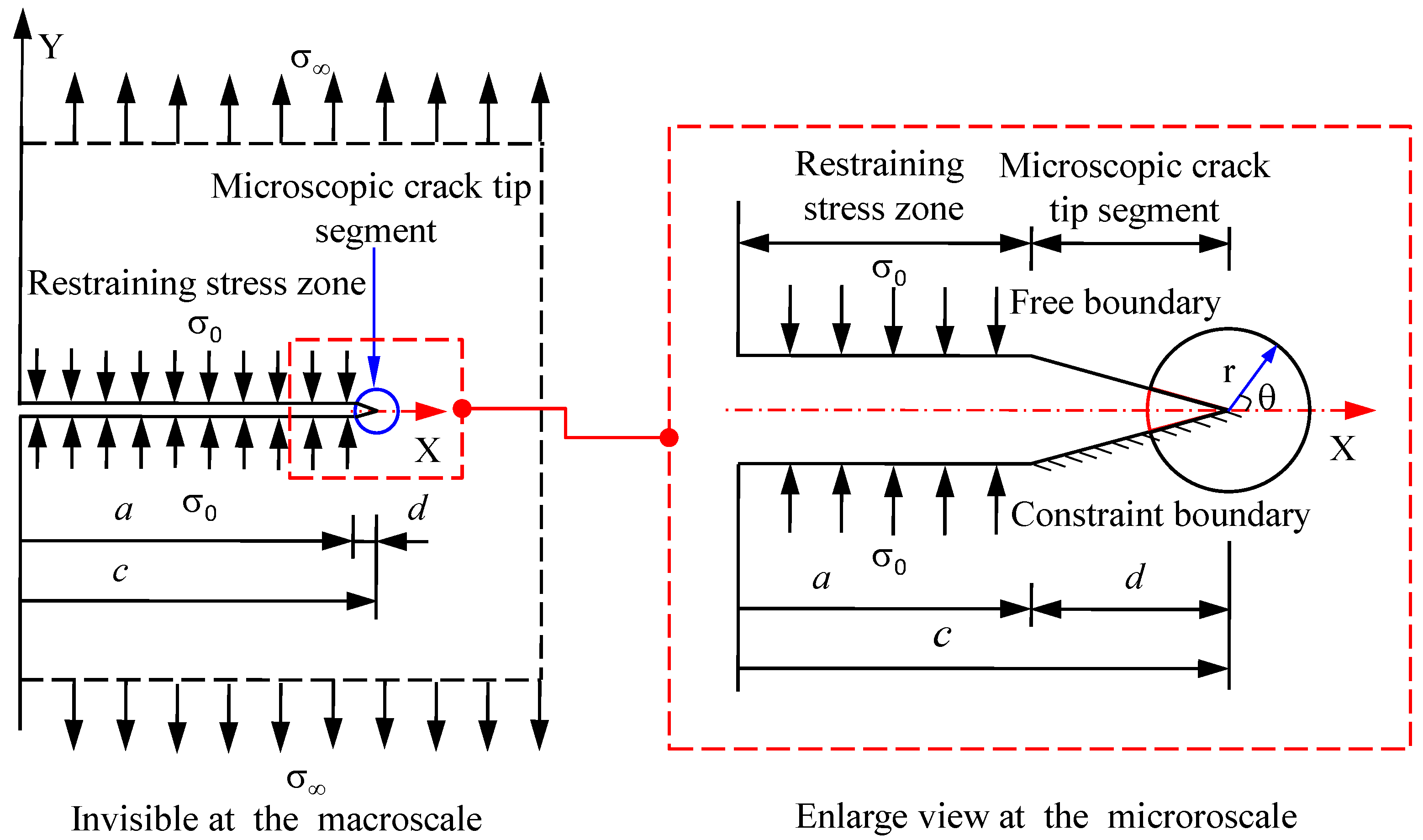
2.1. Macro/Micro Dual Scale Crack Model

In this study, the cracking process is depicted using the macro/micro dual scale crack model, which is based on the concept of restraining stress zone that reflects the material damage. Assuming that a region with the size of a is cut at the fatigue source point, a macro/micro dual scale crack model can be established as shown in Figure 1 [22], where r is a distance measured from the crack tip, and related to the crack propagation segment size at each time. The front of the zone is a V-shape notch which is simplified from the intergranular and transgranular defects with different grain boundary conditions. The restraining stresses would prevail on the cut surfaces denoted by σ₀. The damage degree can be expressed by the ratio of restraining stress to applied stress σ_∞. Initially, the stress ratio σ₀/σ_∞ = 1 when the value of crack size a is very small. As the damage development and the crack size a increase with the cycle number of local load, the stress ratio gradually drops from 1 to 0, indicating the development of a fatigue crack from micro-scale to macro-scale [18]. Hence, the macro/micro dual crack model can describe the total fatigue process from micro to macro scales in a consistent way instead of dividing a continuous fatigue process into two different stages [23].

As wires and cables only bear tension, the tension crack (mode I) is the most common pattern, and, in this study, the stress along the wire (one dimensional) is analyzed for simplicity [22,23,24,25,26,27], though the stress distribution is much more complex with three-dimensional stresses. Furthermore, at the micro scale, the material is anisotropy, while in the analysis at the macro scale, the isotropic elasticity assumption is often used [24]. The material properties may change as the damage develops from micro to macro scale [17,28]. Therefore, different values for the Poisson’s ratio and shear modulus are used at micro and macro scale, respectively. In the macro/micro dual scale crack model, the expression of the macro/micro dual scale strain energy density factor for the tension mode crack can be obtained using Equation (1) [24], where the superscript “macro” and subscript “micro” indicate that $\Delta S_{micro}^{macro}$ is related to both microscopic and macroscopic factors.

$$\Delta S_{micro}^{macro}=a\frac{2\left(1-2{\mathsf{\nu }}_{micro}\right){\left(1-{\mathsf{\nu }}_{macro}\right)}^2{\mathsf{\sigma }}_{\Delta }{\mathsf{\sigma }}_m}{G_{macro}}{G}^{\ast }{\left(1-{\mathsf{\sigma }}^{\ast }\right)}^2\sqrt{\frac{d}{r}},$$

(1)

$$G^{\ast }=\frac{G_{micro}}{G_{macro}},{\mathsf{\sigma }}^{\ast }=\frac{{\mathsf{\sigma }}_0}{{\mathsf{\sigma }}_{\infty }},d=d^{\ast }\cdot d_0,$$

(2)

$${\mathsf{\sigma }}_{\Delta }={\mathsf{\sigma }}_{\text{max}}-{\mathsf{\sigma }}_{\text{min}},{\mathsf{\sigma }}_m=\frac{{\mathsf{\sigma }}_{\text{max}}+{\mathsf{\sigma }}_{\text{min}}}{2}.$$

(3)

v_micro and v_macro are the microscopic and macroscopic Poisson′s ratios, while G_micro and G_macro are the microscopic and macroscopic shear module, respectively. d* is the micro/macro characteristic size ratio, and d is the characteristic size of the local region, which can distinguish the regions of microscopic and macroscopic effects. d₀ is the grain characteristic size of the material, for steel, it can be taken as 10⁻³ mm [25]. σ_∆ and σ_m are the stress range and the mean stress caused by cycle loading, respectively, which can be obtained according to σ_max and σ_min of the stress time-history along the axis of the cable.

2.2. Trans-Scale Formulation for Fatigue Crack Growth of Steel Wire

Previous studies [23,29,30] showed that the fatigue crack in steel wires initially has a circular front and then gradually changes to a straight line crack front and finally fractures without necking effect, exhibiting the brittle characteristics. In spite of the surface effect, a simplified crack model with an equivalent straight front in instead of clam-shell configuration shown in Figure 2 is adopted, according to the assumption that the crack depths in the direction of crack propagation are the same. The equivalent edge crack depth a_c will remain the same as the crack size a. Hence, according to the dual scale fatigue edge crack model, the fatigue crack growth rate da/dN from micro to macro can be described through the following Equation [24]:

$$\frac{da}{dN}=B{\left(\Delta S_{micro}^{macro}\right)}^m,$$

(4)

where N stands for the number of load cycle. B and m are two material fatigue parameters, which can be obtained from laboratory tests. Figure 3 shows the relation between da/dN and ΔK (the amplitude of stress intensity factor) for high strength galvanized steel wires in logarithmic coordinate system, ignoring the mean stress effect, where trans-dimension effect is represented through a straight line [29]. Based on the method in [30], the crack growth rate da/dN can be substituted into the logarithmic form of Equation (4), and B can be determined according to the slope in Figure 3. For the high strength steel wire, m is approximately equal to 1 [30].

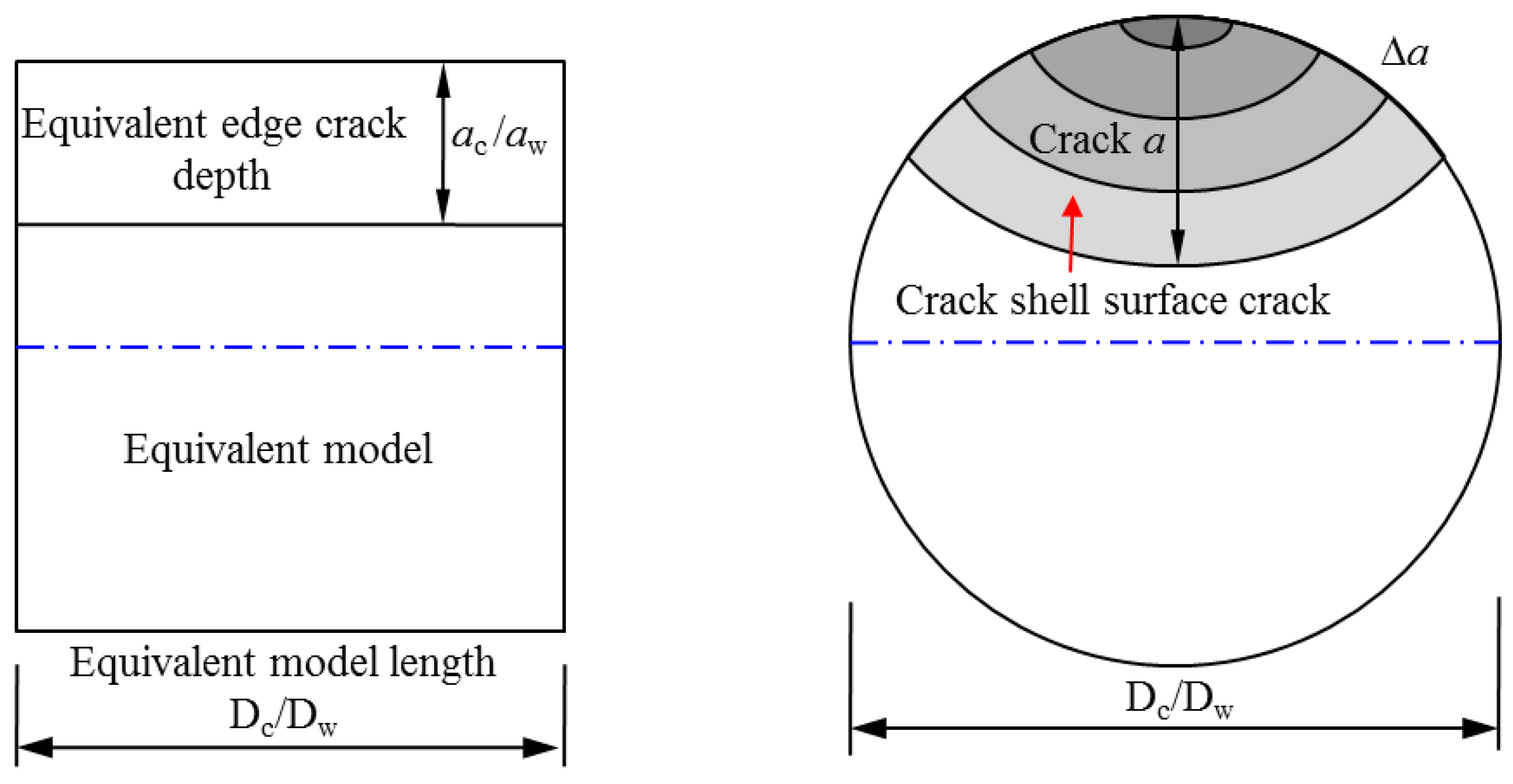
2.3. Fatigue Crack Growth of Cable

A cable is comprised of strands of steel wires wrapping in polymeric tubes with spacing filled by polymers and matrix. Since the cable is no longer homogeneous, the crack growth should be distinguished from that in the steel wire; therefore, extension of the crack growth model in steel wires is needed. In this study, the differences in material properties and strengths between cables and wires are considered. The fatigue crack growth with depth a in a cable can be depicted by Equation (4), while the values of B and m are different from those for steel wires. In addition, σ_∆ and σ_m should be obtained using the rain-flow counting [31], based on the stress time-histories of cables due to random vehicle loads.

Assuming that the material and geometric parameters are fixed [32], as shown in Equation (5), the crack profile is simplified with an equivalent straight front shown in Figure 2. The relationship between a and N can be computed for m = 1 by integrating Equation (4), as shown in Equation (6).

$$G^{\ast }=\frac{G_{macro}}{G_{micro}}=2,{\mathsf{\sigma }}^{\ast }=\frac{{\mathsf{\sigma }}_0}{{\mathsf{\sigma }}_{\infty }}=0.3,d^{\ast }=\frac{d_0}{d_{\infty }}=1,\frac{d_0}{r}=1,{\mathsf{\nu }}_{micro}=0.4,$$

(5)

$$\text{ln}\left[a\left(N\right)\right]=B\frac{0.392{\left(1-{\mathsf{\nu }}_{macro}\right)}^2{\mathsf{\sigma }}_{\Delta }{\mathsf{\sigma }}_m}{G_{macro}}\left(N-N_0\right).$$

(6)

As a result, a can be expressed as follows [33],

$$a\left(N\right)=a_0{e}^{B\frac{0.392{\left(1-{\mathsf{\nu }}_{macro}\right)}^2{\mathsf{\sigma }}_{\Delta }{\mathsf{\sigma }}_m}{G_{macro}}\left(N-N_0\right)},$$

(7)

where a₀ and N₀ are the depth and cycle number of the initial crack, and the initial value follows the normal distributions, with a mean value and deviation of 0.01 mm and 0.012 mm [29,34], respectively, and Nr = N − N₀. B and v_micro can be taken as 1.06 × 10⁻⁶ and 0.3, respectively [35]. According to the elastic mechanics, the following relationship presented in Equation (8) is adopted between shear modulus and elastic modulus:

$$G_{macro}=\frac{E_c}{2\left(1+{\mathsf{\nu }}_{macro}\right)}.$$

(8)

To consider the influence of composite construction on the elastic modulus of the cable, the following Equation (9) is adopted [36]:

$$E_c=\mathsf{\beta }E,\mathsf{\beta }\le 1.0,$$

(9)

where E is the elastic modulus of steel wire and β can be taken as 0.81 [37].

Consequently, Equation (10) can be obtained as follows

$$a\left(N_r\right)=a_0{e}^{B\frac{0.555{\mathsf{\sigma }}_{\Delta }{\mathsf{\sigma }}_m}{E_c}{N}_r}.$$

(10)

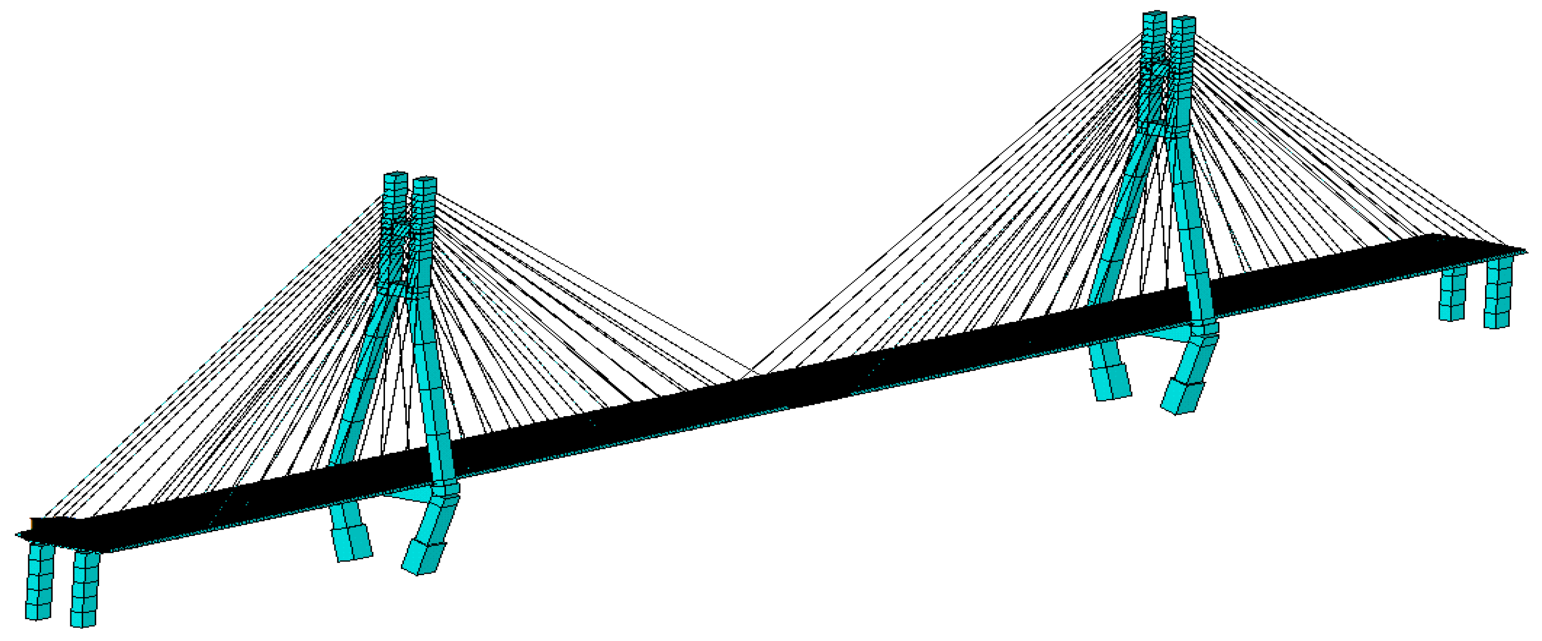
3. FE Modeling of the Runyang Cable-Stayed Bridge

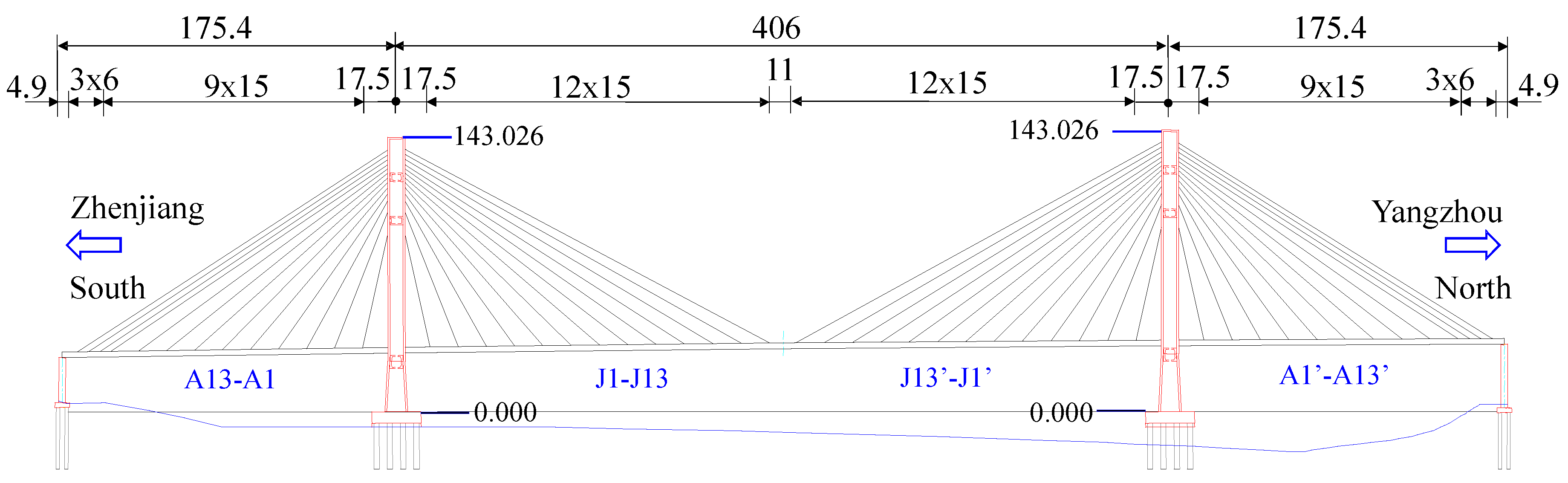
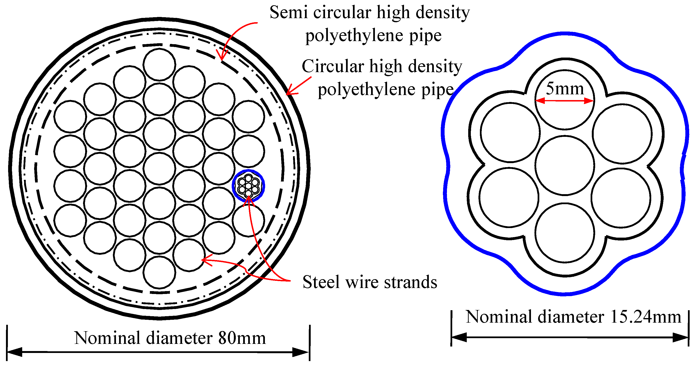
3.1. Bridge Description

The Runyang Bridge, open to traffic in 2005, consists of a suspension bridge (with a main span of 1490 m) and a cable-stayed bridge (175.4 m + 406 m + 175.4 m), as shown in Figure 4. The RCB has a streamlined, closed, flat, steel-box girder supported by 52 cables on each side. The cables consist of unbounded high-strength parallel strands coated by double synchronous extrusion high-density polyethylene (HDPE) protection tubes, as shown in Figure 5. Each cable has a nominal diameter of 80 mm, consisting of 37 steel strands, and the section area of the cable is 5.02 × 10⁻³ m². The nominal fracture strength of the steel strand is no less than 1860 MPa consisting of seven steel wires, whose nominal diameter is 5 mm and the elastic modulus is 1.998 × 10⁵ MPa.

3.2. FE Modeling

In order to investigate the fatigue behavior of cables of the bridge, a FE model of the RCB is developed using the FE program ANSYS (Version 12.0, ANSYS, Inc.: Drive Canonsburg, PA, USA, 2009) [13], as shown in Figure 6. The towers are modeled using the 3D iso-parametric beam elements (i.e., the Beam4 element in ANSYS) having six degrees of freedom (DOFs) at each node. The stayed-cables are modeled using the 3D linear elastic link elements (i.e., the Link10 element) with three DOFs for each node. Those link elements are defined to bear tension only. The cable stresses in the equilibrium configuration are input in terms of initial strains. The material properties and real constants (i.e., areas of cross-section, moments of inertia, etc.) are strictly calculated and assigned to the corresponding elements. The box girders are modeled using shell elements (i.e., the Shell181 element). To reduce the number of elements, the orthotropic decks and bottom plates of the girder are modeled respectively using a layer of plates without U-ribs, and these plates are assigned with orthotropic material properties. However, the decks near the mid-span are refined, so as to facilitate the application of moving loads at the mid-span. The beam188 elements are used simulating the braced truss diaphragms. The concrete and steel blocks, placed inside the box-girders at two side spans to adjust the configuration of the bridge, are modeled using the Mass21 element. Each end of the girder is coupled with one tower cross-beams, except that the longitudinal displacement is free. During the analysis, the large-deflection effect option is selected.

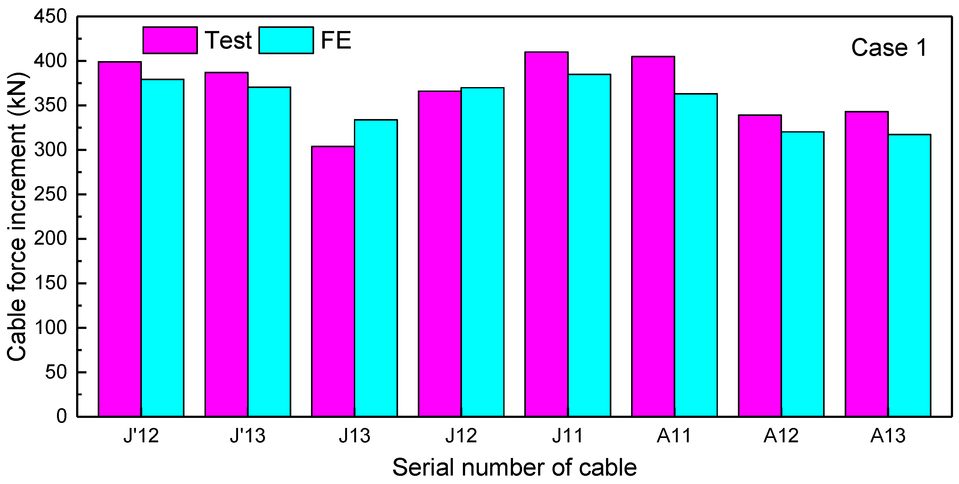
3.3. Validation of FE Model

First, the cable forces under gravity load are calculated and are compared with the test results (half bridge), as shown in Figure 7, where good agreement is observed, showing the effectiveness of the FE model. It is worth noting that the forces of cables near piers, pylons and mid-span are relatively larger. Note that the cables in Figure 4 are labeled from “Zhenjiang” to the south tower as A13, A12, ..., and A1, from the south tower to mid-span as J1, J2, ..., and J13, from mid-span to the north tower as J1′, J2′, ..., and J13′, from the north tower to “Yangzhou” as A1′, A2′, ..., and A13′, respectively.

In addition, one static load case (i.e., load case 1) in the completion test of the bridge, as shown in

Table 1. Description of load case 1.

Load Test	Truck Positions	Illustration	Truck Configuration
Case 1	Sixteen trucks, symmetrically loaded at the mid-span in 4 lines and 4 rows

, is randomly selected to further validate the force increments under vehicle loads. As shown in Figure 8, the calculated force increments, especially for the long cables near piers and mid-span are in good agreement with the measured ones.

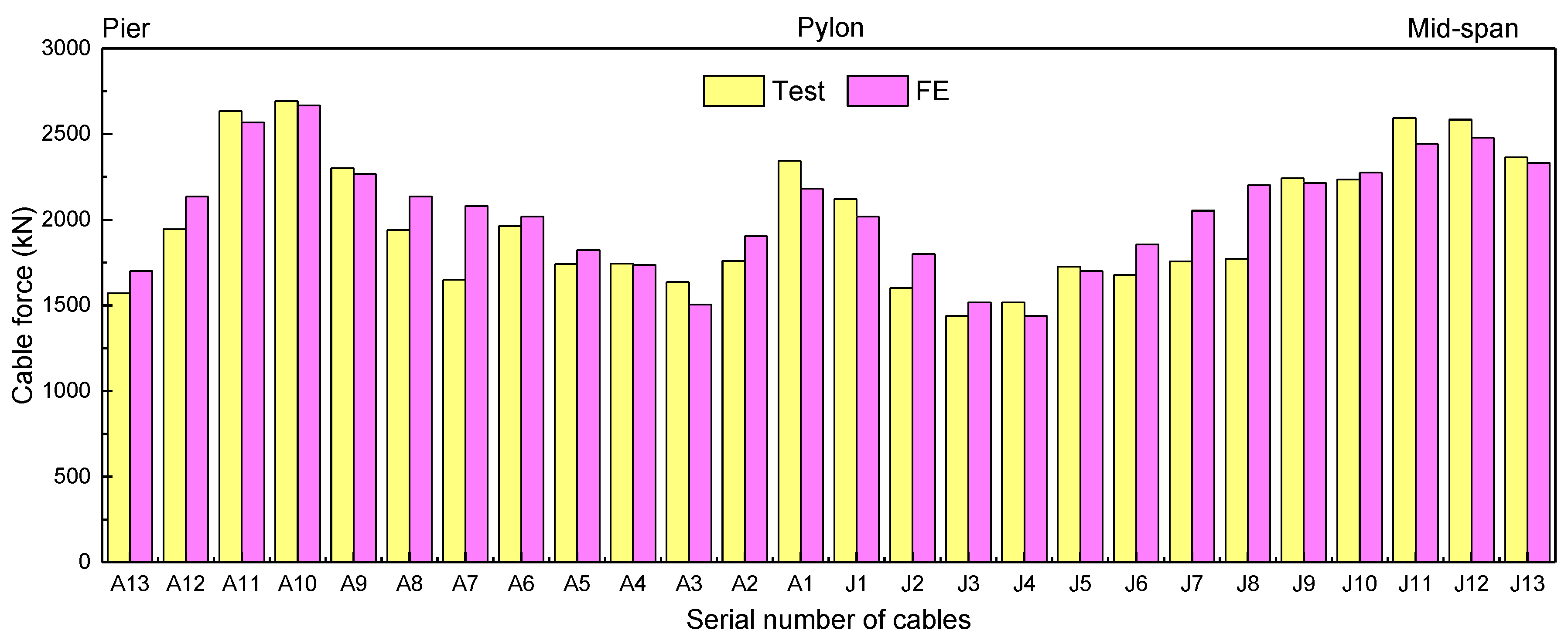
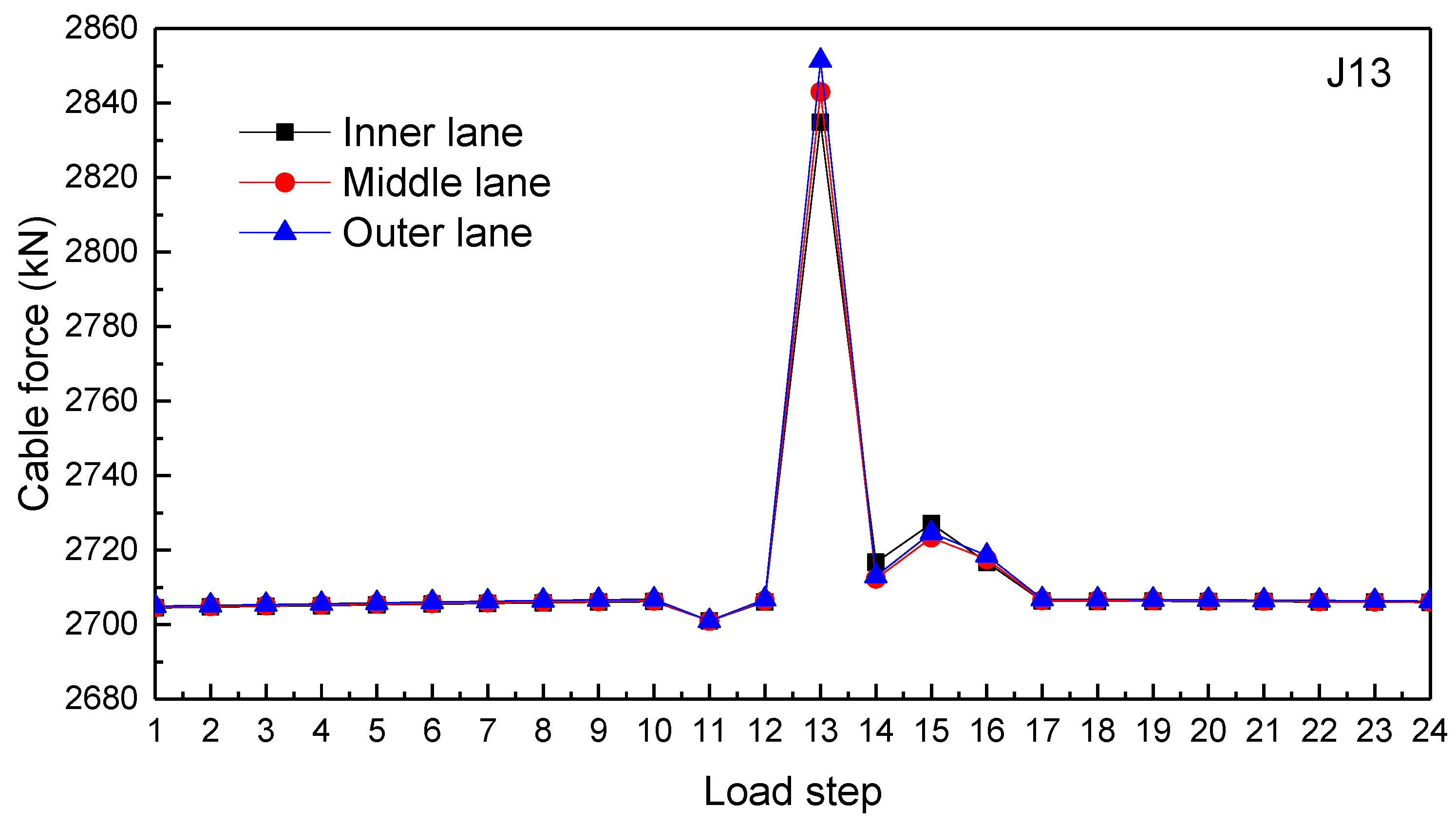
3.4. Force Analysis in Cables

Figure 9 further shows the force time-histories of the cable J13 (randomly selected), when a truck in case 1 is traveling in different lanes. It is observed that the cable force is influenced by the passing truck within a distance of about 52.5 m, especially within 15 m. Transversally, though in general the force responses are similar, the peak values are larger when the truck is in outer and middle lanes than in the inner lane. Therefore, for accurate evaluation of cable life, transversal and longitudinal positions of the cable should be considered.

4. Fatigue Life Prediction of Bridge Cables

4.1. Vehicle Load Model

According to the records from toll stations of the RCB [13], there were a total of 371,167 vehicles passing through the bridge during 28 July 2011 to 31 August 2011. Information including the types of vehicles, number of vehicles in each type, number of axles, and axle weights, etc., is obtained and analyzed. Taking the probabilistic properties of axle weights for example, as summarized in

Table 2. Probabilistic properties of axle weights (dimensions in kN).

Vehicle Type	Graphic Illustration	Variable Designation	Distribution Type	Mean Value	Standard Deviation
1		AW11	Lognormal	10.54	3.12
		AW12	Lognormal	8.55	3.27
2		AW21	Normal	48.29	14.22
		AW22 = AW23	Normal	78.54	36.48
3		AW31	Normal	38.16	10.39
		AW32	Normal	35.66	12.87
		AW33	Lognormal	115.10	65.54
4		AW41	Normal	46.26	10.03
		AW42	Lognormal	52.40	15.50
		AW43 = AW44	Normal (0.18)	33.83	5.70
			Normal (0.82)	82.30	29.84
5		AW51	Lognormal	48.46	6.33
		AW52	Normal (0.23)	43.56	3.29
			Normal (0.37)	74.01	24.03
			Normal (0.4)	132.12	18.12
		AW53 = AW54 = AW55	Normal (0.27)	22.96	1.71
			Normal (0.30)	52.23	13.92
			Normal (0.43)	83.35	9.51
6		AW61	Lognormal	53.86	5.95
		AW62 = AW63	Normal (0.13)	35.35	4.79
			Normal (0.87)	82.17	15.62
		AW64 = AW65 = AW66	Normal (0.07)	22.68	3.20
			Normal (0.16)	38.11	13.95
			Normal (0.77)	80.94	13.11

, there are mainly six types of vehicles crossing the bridge, and the axle weights of most types of vehicles are described by a single-peak probability density function (PDF); however, for the last three types, multi-peaks exist in the PDFs, and therefore, a weighted sum of PDFs are used to describe such distributions.

Using the video camera, the transversal positions (i.e., outer lane, middle lane or inner lane) are also identified, as shown in

Table 3. Constitution of vehicles.

Vehicle Type	Percentage in Traffic Volume (%)	Percentage in Each Lane (%)
		Outer Lane	Middle Lane	Inner Lane
1	76.66	9.70	25.74	41.23
2	0.65	0.36	0.26	0.03
3	1.57	0.60	0.87	0.10
4	1.64	0.92	0.67	0.04
5	2.54	1.31	1.17	0.06
6	16.94	8.43	7.94	0.57

. It is observed that 36.65 percent and 42.03 percent vehicles ran in the middle lane and inner lane (i.e., the fast lane), respectively; whereas 21.32 percent vehicles ran in the outer lane (i.e., the slow lane). For the vehicle type 1 for light weight, most of them (i.e., 41.23 percent) were in the fast lane, and only 9.7 percent were in the slow lane. However, for the vehicle type 6 with heavy weight, their lane occupation was just opposite to that of vehicle type 1. Most heavy trucks were in the middle lane and the slow lane, while only a small portion of them were in the fast lane.

4.2. Fatigue Analysis Approach

To obtain probabilistic distributions of σ_mσ_∆ and Nc, an analysis approach is developed in the MATLAB (Version R2009a, MathWorks, Inc.: Apple Hill Drive Natick, MA, USA, 2009) environment and is outlined as follows:

(1)

According to the vehicle load model in Table 2 and Table 3, a series of vehicles are generated according to the distribution of the vehicle type, the transversal position of vehicle loads, axle loads and the axle spacing by using the truncated Latin Hypercube sampling (LHS) [38] or random sampling.

(2)

According to the vehicle parameters determined in the above step, loads of a given vehicle are applied on the FE model in ANSYS. Each load step corresponds to a static FE analysis, and after each load step, the loads move forward to simulate the movement of the vehicle. Thereafter, the stress time-histories of a particular vehicle can be obtained.

(3)

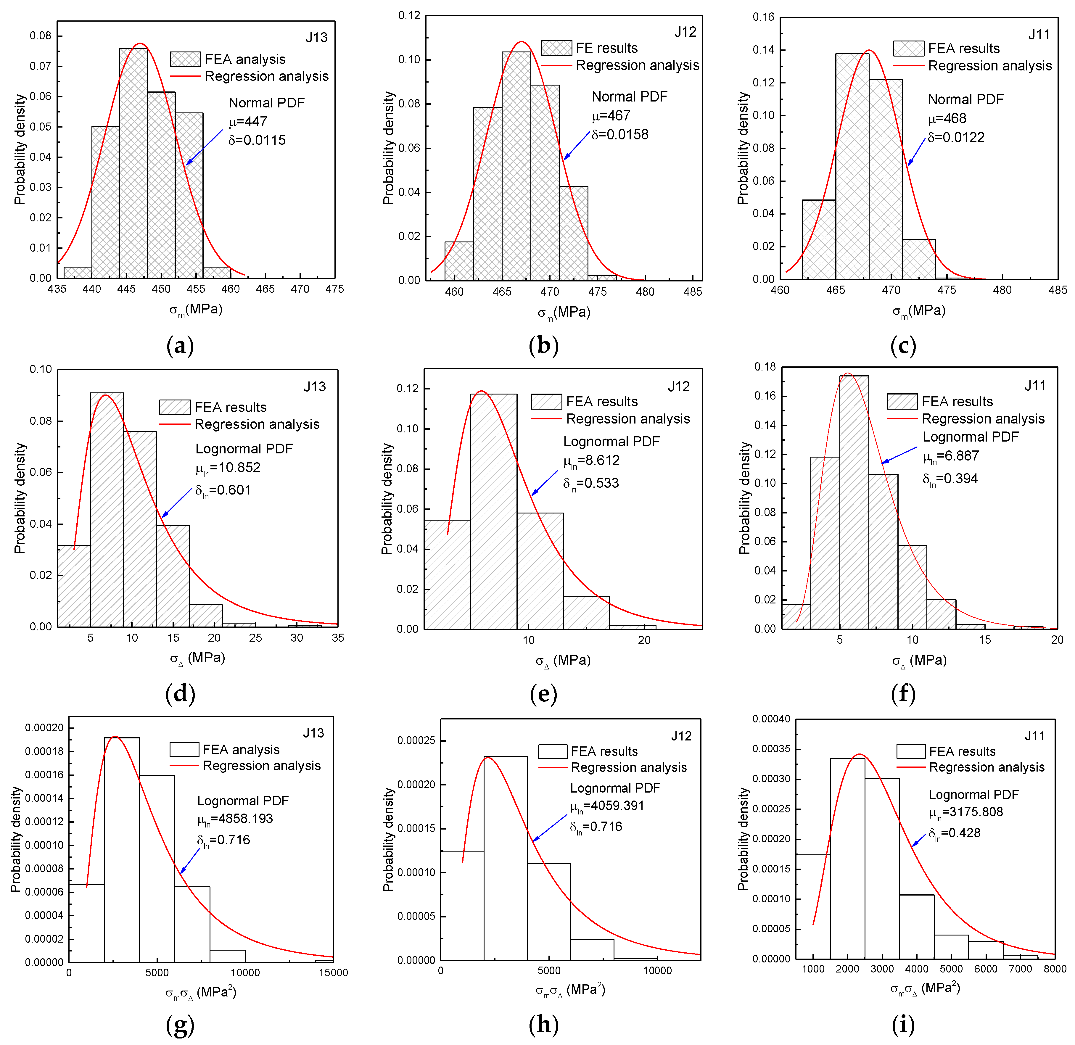
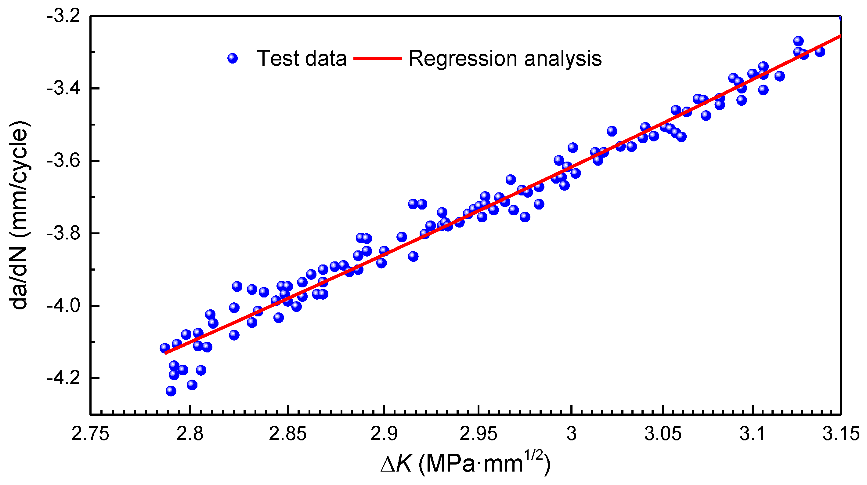
Rain-flow counting [31] is conducted to obtain the mean stresses, the stress ranges and the corresponding number of cycles; after that, regression analysis is performed to obtain the PDFs of σ_mσ_∆.

(4)

According to Equations (9) and (10), the fatigue life can be calculated as follows:

$$T=\frac{N_r}{365\times ADV\times Nc}=\left[\frac{1.805E\text{ln}\left(a_{cr}/a_0\right)}{B{\left(1+DLA\right)}^2{\mathsf{\sigma }}_m{\mathsf{\sigma }}_{\Delta }}\right]/\left(365\times ADV\times Nc\right),$$

(11)

where T is the fatigue life (in year) and ADV represents the number of average daily vehicles. DLA is the coefficient of dynamic load amplification, which has a mean value of 0.057 and the COV of 0.8 [39]. The critical depth of crack, a_cr, is calculated according to the critical wire broken rate of a cable, which follows a normal distribution with the mean value of 4mm in this study [40]. Considering the high level of uncertainty of material properties, B and E are treated as random variables, with their probabilistic properties listed in

Table 4. Random variables used in fatigue reliability analyses.

Variable Designation	Meaning of Variable	Distribution Type	Mean Value	COV	Source
B	Fracture parameter	Lognormal	1.06 × 10−6	0.63	Fisher [41]
E	Young’s modulus	Lognormal	2.0 × 105 MPa	0.05	Elachachi et al. [20]
a0	Initial crack depth	Normal	0.01 mm	1.2	Mahmoud [29]; Molent [34]
ac	Critical crack depth	Normal	4 mm	0.2	MCCHSRI [40]
DLA	Dynamic load amplification factor	Normal	0.057	0.8	AASHTO [39]; NCHRP [42]

.

4.3. Results and Discussion

According to the above analysis method, the probabilistic distributions of σ_m, σ_∆ and σ_mσ_∆ of cables J13, J12 and J11 are obtained, as shown in Figure 10, where it is observed that these distributions can be represented through normal or lognormal PDFs. Compared with cables J11 and J12, the longer cable J13 may have a slightly smaller mean stress, which is consistent with the calculated and measured results in Figure 7, while it is subjected to larger stress range. Based on the PDFs of σ_mσ_∆ and the probabilistic distributions of Nc, the probabilistic fatigue lives of the cables J13, J12 and J11 are obtained using Equation (12) from

Table 5. Predicted fatigue lives of cables.

Serial Number of Cables	σmσ∆ (MPa2)		T (year)
	μln	δln	μ	σ
J13	4858.193	0.716	29.11	10.32
J12	4059.391	0.716	34.85	13.15
J11	3175.808	0.428	44.54	17.47

, and it is observed that the mean lives of cables are 29.11, 34.85 and 44.54 years, respectively. However, the standard deviation of fatigue lives of the three cables are considerable, being 10.32, 13.15 and 17.47 years, respectively, indicating that there are high possibilities for the cables to have a shorter life than designed (i.e., 30 years). It is also observed from Figure 10 that longer cables show shorter lifetime, and one reason is that in the Runyang Cable-Stayed Bridge, longer cables are subjected to larger loads, resulting in larger stress amplitudes, as shown in Figure 10d–f. It is also worth noting that in material engineering, a specimen with longer length has a shorter lifetime due to the higher probability of having a weaker link [43].

5. Conclusions

This paper presents the probabilistic fatigue life prediction of bridge cables based on multiscaling and mesoscopic fracture mechanics. According to the methodologies and assumptions adopted in this paper, the following conclusions are drawn.

• Fatigue crack growth in stay cables is a multiscale process, influenced not only by the initial defects, material properties, and also by some global parameters, such as cable length, mean stress, longitudinal position and vehicle loads, etc. According to the FE analysis, long cables near bridge piers, pylons and mid-span may be more prone to fatigue than the others, and transversal positions of vehicles may influence the cable force, which calls for a more comprehensive vehicle load model including lane occupation.
• The fatigue crack growth, on the other hand, abounds with uncertainties, so that a probabilistic analysis approach is proposed, which is based on a probabilistic vehicle load model, finite element analysis and multiscaling and mesoscopic fracture mechanics. The proposed uncertain parameters, with their probabilistic properties, are defined and a demonstration study is made.
• According to the probabilistic FE analyses, the mean lives of the three cables are ranging from 29.11 to 44.54 years; however, the standard deviation of fatigue lives of the three cables are considerable, indicating that there are high possibilities for the cables to have a shorter life than designed.

References

1. Ren, W.X. Ultimate behavior of long-span cable-stayed bridges. J. Bridge Eng. 1999, 4, 30–37. [Google Scholar] [CrossRef]
2. Xie, X.; Li, X.Z.; Shen, Y.G. Static and dynamic characteristics of a long-span cable-stayed bridge with CFRP cables. Materials 2014, 7, 4854–4877. [Google Scholar] [CrossRef]
3. Li, S.L.; Xu, Y.; Zhu, S.Y.; Guan, X.C.; Bao, Y.Q. Probabilistic deterioration model of high-strength steel wires and its application to bridge cables. Struct. Infrastruct. Eng. 2015, 11, 1240–1249. [Google Scholar] [CrossRef]
4. Pipinato, A.; Pellegrino, C.; Fregno, G.; Modena, C. Influence of fatigue on cable arrangement in cable-stayed bridges. Int. J. Steel Struct. 2012, 12, 107–123. [Google Scholar] [CrossRef]
5. Li, H.; Lan, C.M.; Ju, Y.; Li, D.S. Experimental and numerical study of the fatigue properties of corroded parallel wire cables. J. Bridge Eng. 2011, 17, 211–220. [Google Scholar] [CrossRef]
6. Stallings, J.M.; Frank, K.H. Stay-cable fatigue behavior. J. Struct. Eng. 1991, 117, 936–950. [Google Scholar] [CrossRef]
7. Mehrabi, A.B.; Ligozio, C.A.; Ciolko, A.T.; Scott, T.W. Evaluation, rehabilitation planning, and stay-cable replacement design for the hale Boggs Bridge in Luling, Louisiana. J. Bridge Eng. 2010, 15, 364–372. [Google Scholar] [CrossRef]
8. Nowak, A.S.; Hong, Y.K. Bridge live-load models. J. Struct. Eng. 1991, 117, 2757–2767. [Google Scholar] [CrossRef]
9. Guo, T.; Frangopol, D.M.; Chen, Y.W. Fatigue reliability assessment of steel bridge details integrating weigh-in-motion data and probabilistic finite element analysis. Comput. Struct. 2012, 112, 245–257. [Google Scholar] [CrossRef]
10. Basso, P.; Casciati, S.; Faravelli, L. Fatigue reliability assessment of a historic railway bridge designed by Gustave Eiffel. Struct. Infrastruct. Eng. 2015, 11, 27–37. [Google Scholar] [CrossRef]
11. Kwon, K.; Frangopol, D.M. Bridge fatigue reliability assessment using probability density functions of equivalent stress range based on field monitoring data. Int. J. Fatigue 2010, 32, 1221–1232. [Google Scholar] [CrossRef]
12. Maljaars, J.; Vrouwenvelder, T. Fatigue failure analysis of stay cables with initial defects: Ewijk bridge case study. Struct. Saf. 2014, 51, 47–56. [Google Scholar] [CrossRef]
13. Guo, T.; Liu, Z.X.; Zhu, J.S. Fatigue reliability assessment of orthotropic steel bridge decks based on probabilistic multi-scale finite element analysis. Adv. Steel Constr. 2015, 11, 334–346. [Google Scholar]
14. Gu, M.; Xu, Y.L.; Chen, L.Z.; Xianga, H.F. Fatigue life estimation of steel girder of Yangpu cable-stayed bridge due to buffeting. J. Wind Eng. Ind. Aerodyn. 1999, 80, 383–400. [Google Scholar] [CrossRef]
15. Llorca, J.; Sánchez-Gálvez, V. Fatigue limit and fatigue life prediction in high strength cold drawn eutectoid steel wires. Fatigue Fract. Eng. Mater. Struct. 1989, 12, 31–45. [Google Scholar] [CrossRef]
16. Razmi, J. Fracture mechanics-based and continuum damage modeling approach for prediction of crack initiation and propagation in integral abutment bridges. J. Comput. Civ. Eng. 2015. [Google Scholar] [CrossRef]
17. Ladani, L.J. Successive softening and cyclic damage in viscoplastic material. J. Electron. Packag. 2010, 132. [Google Scholar] [CrossRef]
18. Chookah, M.; Nuhi, M.; Modarres, M. A probabilistic physics-of-failure model for prognostic health management of structures subject to pitting and corrosion-fatigue. Reliab. Eng. Syst. Saf. 2011, 96, 1601–1610. [Google Scholar] [CrossRef]
19. Zhu, S.P.; Huang, H.Z.; Ontiveros, V.; He, L.P.; Modarres, M. Probabilistic low cycle fatigue life prediction using an energy-based damage parameter and accounting for model uncertainty. Int. J. Damage Mech. 2011. [Google Scholar] [CrossRef]
20. Elachachi, S.M.; Breysse, D.; Yotte, S.; Cremona, C. A probabilistic multi-scale time dependent model for corroded structural suspension cables. Probab. Eng. Mech. 2006, 21, 235–245. [Google Scholar] [CrossRef]
21. Li, C.X.; Tang, X.S.; Xiang, G.B. Fatigue crack growth of cable steel wires in a suspension bridge: Multiscaling and mesoscopic fracture mechanics. Theor. Appl. Fract. Mech. 2010, 53, 113–126. [Google Scholar] [CrossRef]
22. Sih, G.C.; Tang, X.S. Asymptotic micro-stress field dependency on mixed boundary conditions dictated by micro-structural asymmetry: Mode I macro-stress loading. Theor. Appl. Fract. Mech. 2006, 46, 1–14. [Google Scholar] [CrossRef]
23. Toribio, J.; Matos, J.C.; González, B. Micro-and macro-approach to the fatigue crack growth in progressively drawn pearlitic steels at different R-ratios. Int. J. Fatigue 2009, 31, 2014–2021. [Google Scholar] [CrossRef]
24. Sih, G.C.; Tang, X.S. Micro/macro-crack growth due to creep-fatigue dependency on time-temperature material behavior. Theor. Appl. Fract. Mech. 2008, 50, 9–22. [Google Scholar] [CrossRef]
25. Tang, X.S.; Wei, T.T. Microscopic inhomogeneity coupled with macroscopic homogeneity: A localized zone of energy density for fatigue crack growth. Int. J. Fatigue 2015, 70, 270–277. [Google Scholar] [CrossRef]
26. Tang, K.K. Reliability of micro/macro-fatigue crack growth behavior in the wires of cable-stayed bridge. In Proceedings of the 13th International Conference on Fracture, Beijing, China, 16–21 June 2013.
27. Tang, X.S.; Peng, X.L. An energy density zone model for fatigue life prediction accounting for non-equilibrium and non-homogeneity effects. Theor. Appl. Fract. Mech. 2015, 79, 105–112. [Google Scholar] [CrossRef]
28. Kachanov, M.; Sevostianov, I. On quantitative characterization of microstructures and effective properties. Int. J. Solids Struct. 2005, 42, 309–336. [Google Scholar] [CrossRef]
29. Mahmoud, K.M. Fracture strength for a high strength steel bridge cable wire with a surface crack. Theor. Appl. Fract. Mech. 2007, 48, 152–160. [Google Scholar] [CrossRef]
30. Sih, G.C. Multiscale Fatigue Crack Initiation and Propagation of Engineering Materials: Structural Integrity and Microstructural Worthiness: Fatigue Crack Growth Behaviour of Small and Large Bodies; Springer: New York, NY, USA, 2008. [Google Scholar]
31. Wirsching, P.H.; Shehata, A.M. Fatigue under wide band random stresses using the rain-flow method. J. Eng. Mater. Technol. 1977, 99, 205–211. [Google Scholar] [CrossRef]
32. Sih, G.C.; Tang, X.S.; Li, Z.X.; Li, A.Q.; Tang, K.K. Fatigue crack growth behavior of cables and steel wires for the cable-stayed portion of Runyang bridge: Disproportionate loosening and/or tightening of cables. Theor. Appl. Fract. Mech. 2008, 49, 1–25. [Google Scholar] [CrossRef]
33. Polák, J.; Zezulka, P. Short crack growth and fatigue life in austenitic-ferritic duplex stainless steel. Fatigue Fract. Eng. Mater. Struct. 2005, 28, 923–935. [Google Scholar] [CrossRef]
34. Molent, L.; Barter, S.A. A comparison of crack growth behaviorin several full-scale airframe fatigue tests. Int. J. Fatigue 2007, 29, 1090–1099. [Google Scholar] [CrossRef]
35. Sih, G.C. Invariant form of micro-/macro-cracking in fatigue. In Structural Integrity and Microstructural Worthiness; Springer: Dordrecht, The Netherlands, 2008; pp. 181–208. [Google Scholar]
36. Sih, G.C.; Tang, X.S. Fatigue crack growth rate of cable-stayed portion of Runyang bridge: Part I—Cable crack growth due to disproportionate cable tightening/loosening and traffic loading. In Multiscale Fatigue Crack Initiation and Propagation of Engineering Materials: Structural Integrity and Microstructural Worthiness; Springer: Dordrecht The Netherlands, 2008; pp. 209–247. [Google Scholar]
37. Fontanari, V.; Benedetti, M.; Monelli, B.D.; Degasperi, F. Fire behavior of steel wire ropes: Experimental investigation and numerical analysis. Eng. Struct. 2015, 84, 340–349. [Google Scholar] [CrossRef]
38. Stein, M. Large sample properties of simulations using Latin hypercube sampling. Technometrics 1987, 29, 143–151. [Google Scholar] [CrossRef]
39. American Association of State Highway and Transportation Officials. Subcommittee on Systems Operations and Management–2008 Strategic Plan; Association of State Highway and Transportation Officials: Washington, DC, USA, 2012. [Google Scholar]
40. MCCHSRI (Ministry of Communications Chongqing Highway Science Research Institute). Technical Conditions for Hot-Extruding PE Protection High Strength Wire Cable of Cable-Stayed Bridge; GB/T 18365–2001; Ministry of Communications Chongqing Highway Science Research Institute: Beijing, China, 2001. [Google Scholar]
41. Fisher, J.W. Fatigue and Fracture in Steel Bridges; Wiley: New York, NY, USA, 1984. [Google Scholar]
42. NCHRP (National Cooperative Highway Research Program). Updating the Calibration Report for AASHTO LRFD Code, 20-07/186; Transportation Research Board, National Research Council: Washington, DC, USA, 2007. [Google Scholar]
43. Faber, M.H.; Engelund, S.; Rackwitz, R. Aspects of parallel wire cable reliability. Struct. Saf. 2003, 25, 201–225. [Google Scholar] [CrossRef]
Figure 1. Macro/micro dual scale crack model. Adapted with permission from [22], Copyright 2006, Elsevier Ltd.
Applsci 06 00099 g001
Figure 2. Crack and equivalent depth of steel wire. Adapted with permission from [30], Copyright 2008, Springer.
Applsci 06 00099 g002
Figure 3. da/dN versus ΔK in logarithmic coordinate system. Reproduced with permission from [30], Copyright 2008, Springer.
Applsci 06 00099 g003
Figure 4. Profile of the Runyang Cable-Stayed Bridge (dimensions in meter).
Applsci 06 00099 g004
Figure 5. Cross-sections of cable and strands.
Applsci 06 00099 g005
Figure 6. FE model of the Runyang Cable-stayed Bridge.
Applsci 06 00099 g006
Figure 7. Comparison between calculated and measured cable forces (under gravity load).
Applsci 06 00099 g007
Figure 8. Calculated and measured force increments of cables (load case 1).
Applsci 06 00099 g008
Figure 9. Force time-histories of the cable J13.
Applsci 06 00099 g009
Figure 10. (ac) probabilistic density functions of σm; (df) probabilistic density functions of σ; (gi) probabilistic density functions of σmσ.
Applsci 06 00099 g010