Probability of Interference-Optimal and Energy-Efficient Analysis for Topology Control in Wireless Sensor Networks

Abstract

Because wireless sensor networks (WSNs) have been widely used in recent years, how to reduce their energy consumption and interference has become a major issue. Topology control is a common and effective approach to improve network performance, such as reducing the energy consumption and network interference, improving the network connectivity, etc. Many topology control algorithms reduce network interference by dynamically adjusting the node transmission range. However, reducing the network interference by adjusting the transmission range is probabilistic. Therefore, in this paper, we analyze the probability of interference-optimality for the WSNs and prove that the probability of interference-optimality increases with the increasing of the original transmission range. Under a specific transmission range, the probability reaches the maximum value when the transmission range is 0.85r in homogeneous networks and 0.84r in heterogeneous networks. In addition, we also prove that when the network is energy-efficient, the network is also interference-optimal with probability 1 both in the homogeneous and heterogeneous networks.

1. Introduction

Wireless sensor networks (WSNs) have been widely used in recent years. The properties of WSNs—which contain hundreds or thousands of nodes—are limited by energy, bandwidth, computing capability, etc. [1,2,3,4]. Interference is an important factor of WSNs, affecting not only the data transmission efficiency, but also the energy consumption. High interference means low communication quality and high energy consumption. In multihop WSNs, due to the characteristics of wireless communication, the network performance is affected by interference more seriously than that of the wired network. On one hand, the node which is receiving data packets will be affected by the nodes with transmission ranges that cover this node; on the other hand, the nodes which are sending data packets will interfere with the nodes that fall into their transmission ranges [5,6]. In addition, high interference causes serious propagation delays and packet retransmissions, which consumes a large amount of energy. At worst, the serious interference can make the network fail to work.

Many algorithms have been proposed to reduce the network interference. One remarkable approach is topology control. The aims of topology control are: improving the network connection and reducing the energy consumption [7,8]. Many remarkable topology control algorithms have been proposed, such as [5,9,10,11,12,13,14,15,16,17,18,19,20]. However, based on the conclusions of [5,6], reducing the transmission range cannot guarantee low network interference, i.e., a small transmission range does not mean small network interference. This property is important. It is necessary to take this property into account when designing the interference-optimal topology control algorithm. However, the related issues shown below have not been analyzed accurately so far:

• What is the probability that the network interference is reduced when adjusting the transmission range?
• What are the properties of this probability, such as how this probability varies when the network topology or the transmission range changes?
• If the network topology is fixed, which transmission range has the highest probability of interference-optimality?
• What is the relationship between the interference-optimal and the energy-efficient, i.e., the probability that the interference-optimality and energy-efficiency can be achieved at the same time?

Therefore, these issues will be investigated and analyzed in detail in this paper.

Motivated by these issues, in this paper, we firstly analyze the probability of interference-optimality by adjusting the transmission ranges. We prove that the probabilities in homogeneous networks and heterogeneous networks are $p_{\mathrm{hom}}$ and $p_{\mathrm{het}}$, respectively. With an increase in node density, this probability increases, too. Moreover, if the transmission range is large enough, when the transmission range reduces, the interference decreases with probability 1. This transmission range is large in sparse network and small in a density network. Secondly, we calculate the probability of interference-optimality under a specific transmission range and find out the optimal transmission range which has the maximum probability of interference-optimality. In homogeneous networks, this probability is $P_{\mathrm{homs}}$ and the optimal transmission range is 0.85r. In heterogeneous networks, this probability will be $P_{\mathrm{hets}}$ and the optimal transmission range is 0.84r. Finally, we investigate the relationship between energy-efficiency and interference-optimality when adjusting the transmission range. We prove that if the network is energy-efficient, the network is also interference-optimal both in the homogeneous and heterogeneous WSNs.

The contributions of this paper are as follows:

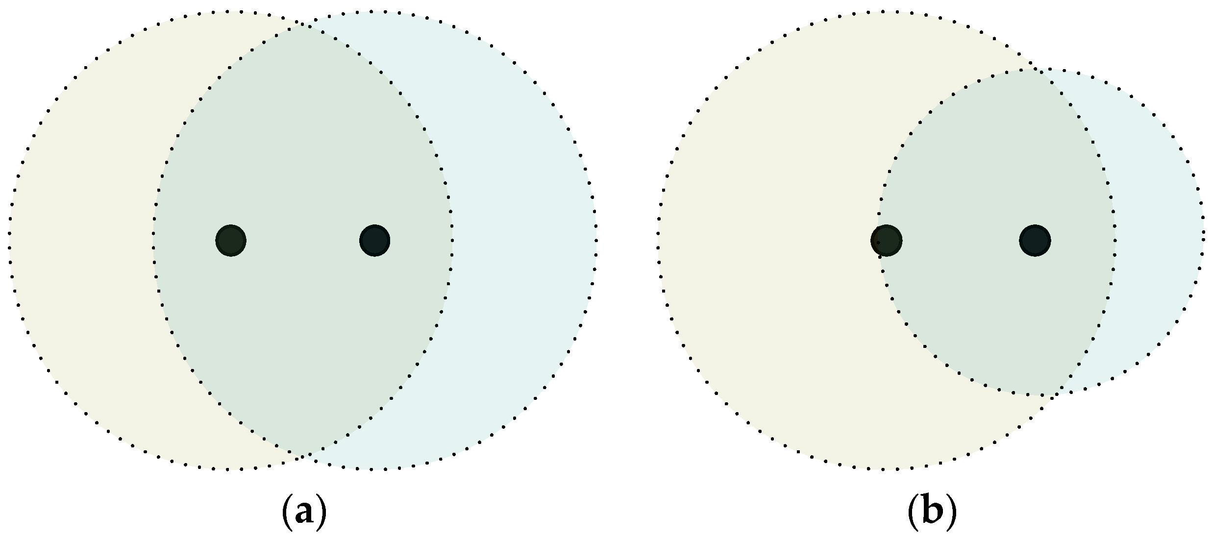
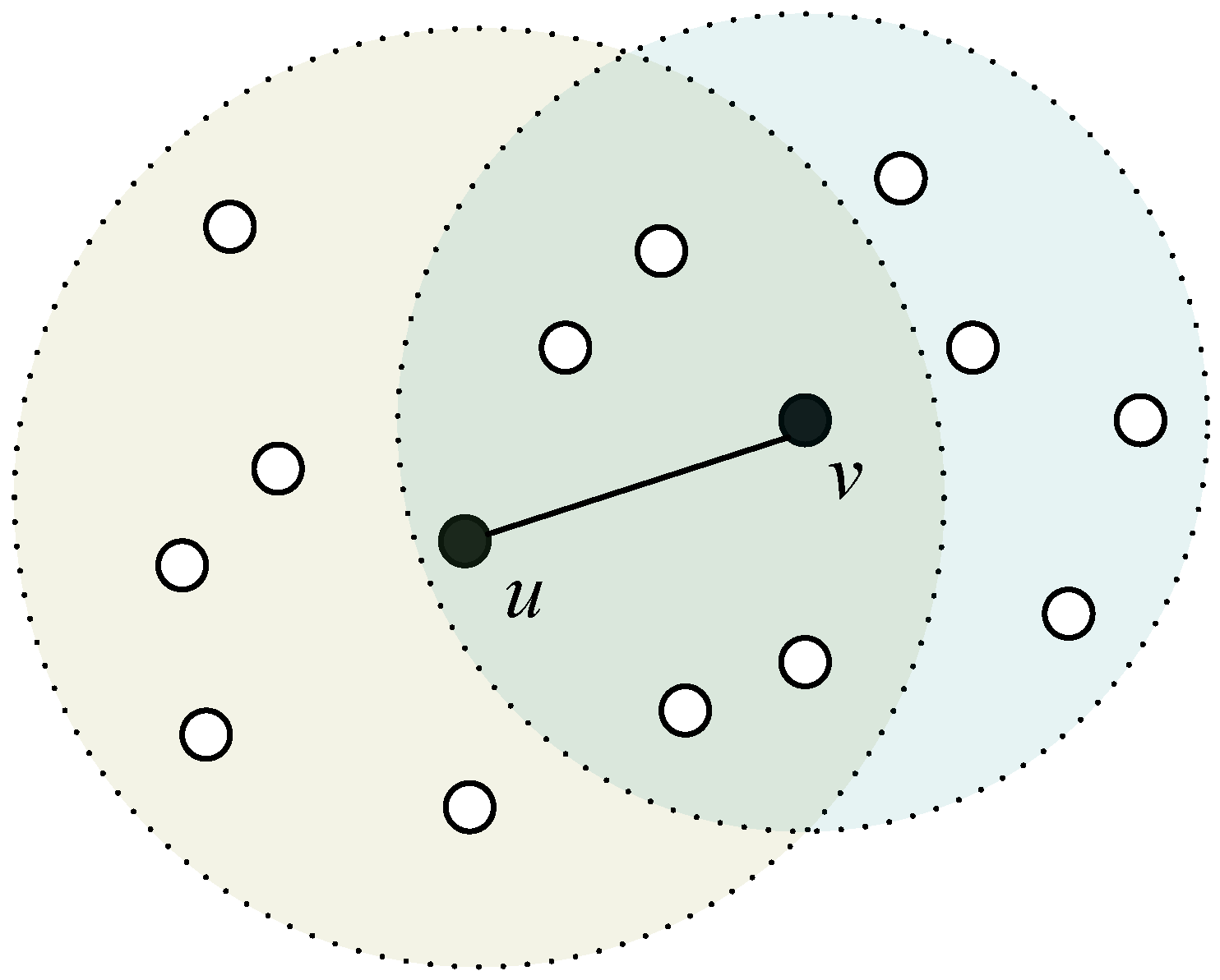
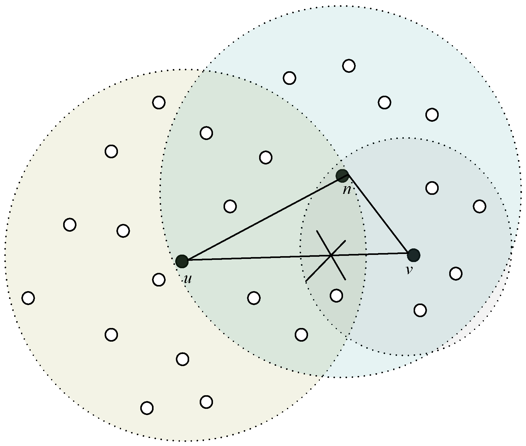
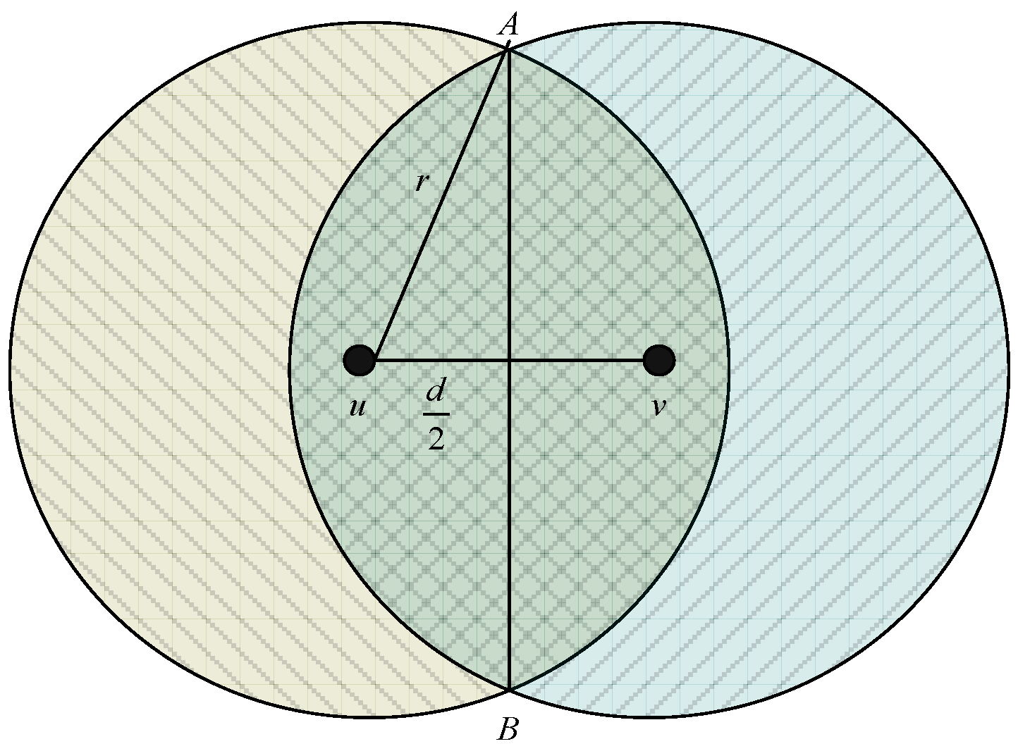
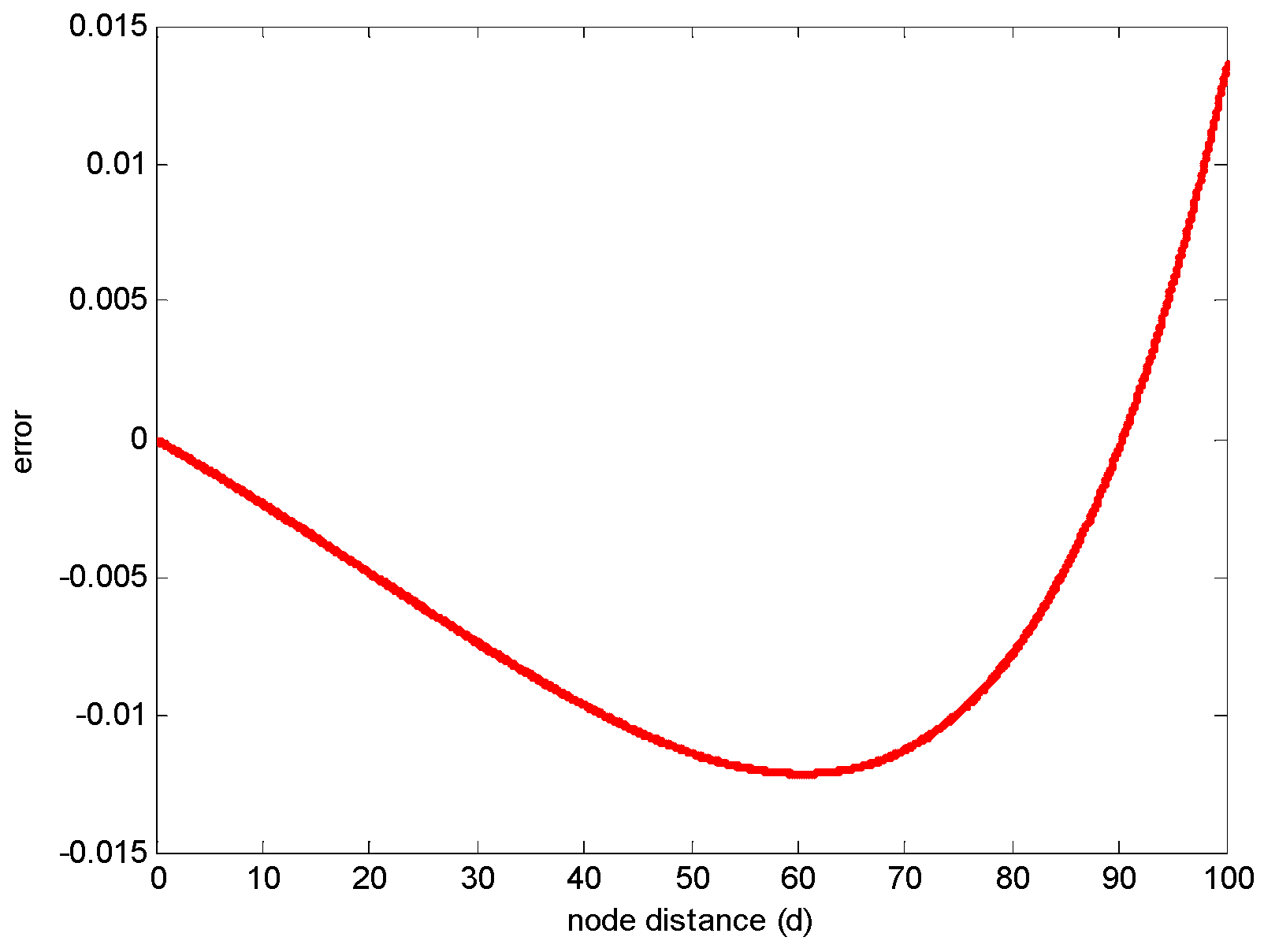
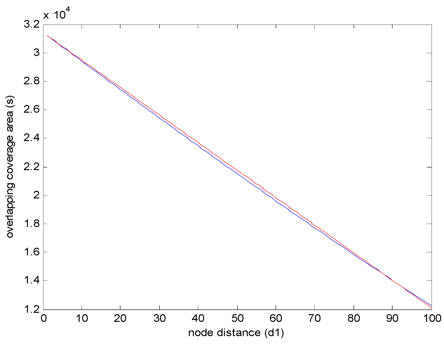
• We explore the relationship between the node distance and the overlapping coverage area of two nodes;
• We analyze the probability of interference-optimality when adjusting the transmission range;
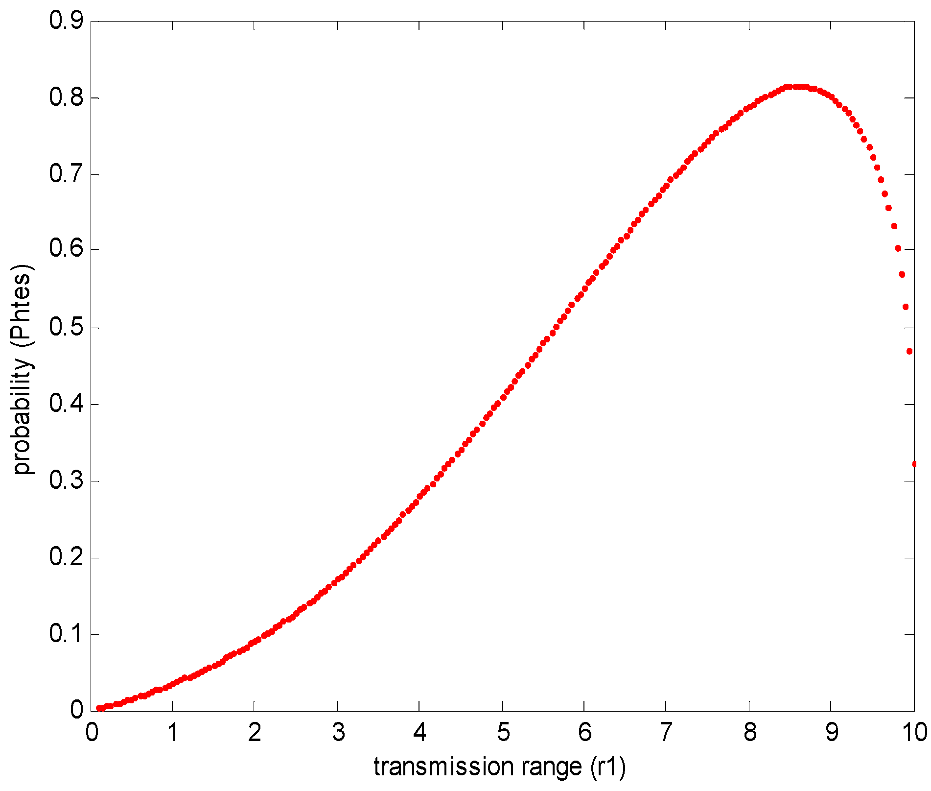
• We calculate the probability of interference-optimality under specific transmission range and find out the optimal transmission range which has maximum probability of interference-optimality;
• We investigate the relationship between energy-efficiency and interference-optimality.

The rest of this paper is organized as follows: in Section 2, we review the related works in recent years; in Section 3, the network model will be introduced; Section 4 analyzes the probability of interference-optimality; Section 5 investigates the relationship between interference-optimality and energy-efficiency; the properties of the probability will be estimated in Section 6; Section 7 concludes our work in this paper.

2. Related Works

There are a large number of researches that have been implemented to reduce the interference in WSNs. In [5,6], first, the authors show that reducing the transmission range cannot guarantee low network interference; then they propose several algorithms to construct topologies in which the maximum link interference is minimized while the network is still connected. In [9], the authors have discussed different methods which are used to measure network interference and proposed a new topology control algorithm to describe the interference of the entire network. The new algorithm minimizes the network interference and successfully maintains the spanner properties of the original network. The work in [10] studies the interference in WSNs and proposes several algorithms to construct topologies such that the maximum node interference and the average node interference are minimized. Based on the Yao Gabriel Graph, the authors propose the SBYaoGG (Smart Boundary Yao Gabriel Graph) algorithm in [11]. The SBYaoGG algorithm tends to produce as sparse a network as possible to meet the objective of high energy efficiency and low interference. In [12], the authors propose an interference-based topology control algorithm for the delay constrained mobile ad hoc network (ITCD). In this algorithm, the impact of node mobility on ITCD is investigated. Moreover, the transmission delay, the contention delay, and the queuing delay are taken into account to remove the unstable communication links. For reducing the link interference in co-channel wireless ad hoc and sensor networks, in [13], the authors propose a new link interference model. Based on this model, a centralized topology control algorithm is designed to construct an interference-optimal network. The new interference model can also be found in [14]. This interference model can not only reflect the fact that interference occurs when the node is receiving a message, but also demonstrates robustness when adding or removing nodes from the network. In [15], the authors investigate how to minimize the average interference when a node is receiving message. In this paper, the 1-D (1-Dimensional) and 2-D (2-Dimensional) networks are studied; and two exact algorithms are proposed to minimize the average interference of 1-D and 2-D networks, respectively. Based on the PRR-SINR (Packet Reception Ratio versus Signal to Interference Plus Noise Ratio) model, in [16], the authors propose an accuracy-aware algorithm for interference modeling and measurement in WSNs. This accuracy-aware algorithm can characterize the accuracy of the PRR-SINR model and enforce a specified accuracy bound by adaptively controlling the measurement process during the run time. In [17], the authors define an explicit notion for network interference and propose an interference model based on the current network traffic. The work in [18] models the interference with physical signal and noise ratio, and defines the concept of scheduling complexity for the wireless network connectivity. In [19], the authors present a comprehensive survey on the interference models for wireless ad hoc networks. The survey emphasizes the domains of the application and illustrates them with examples.

There are also many research papers which are devoted to measuring the interference in WSNs, such as [20,21,22,23]. In [20], the authors take the shadowing and fading effects into account to determine the interference range of the link. The link interference is determined by the interference number which is calculated based on the real coverage region. The interference measurement algorithms also can be found in [21,22]. In [21], a passive interference measurement approach which is derived from the actual physical model has been presented. In [22], the authors propose SoNIC (Sensor Network Interference Classification) to detect interference in an 802.15.4 sensor network which shares 2.4 GHz with other Bluetooth and Wi-Fi devices. The authors in [23] investigate interference prediction in MANETs (Mobile Ad Hoc Networks) (in which the node number is finite) by using a general-order linear model.

However, considering the fact that the topology control algorithms which reduce the network interference by adjusting the transmission range are probabilistic, the related issues that were introduced in Section 1 have not been analyzed accurately by the related works introduced above. This is also the main motivation of this paper.

3. Network Model

In general, there are three models that can express the connection mode between nodes, which are shown in Figure 1 [24]. Figure 1a illustrates the k nearest neighbor model; each node in this model has constant neighbors and can maintain the node degree by changing the communication range of each node. Figure 1b illustrates the disc model. In this model, transmission range is modeled as a disk with radius r; nodes connect with the neighbors that fall into its transmission range. The disc model is more plausible in the WSNs since obtaining k neighbors is not always feasible due to the communication range limitation. In Figure 1c illustrates the Erdos-Renyi random graph that connects any two nodes with the same probability which is not appropriate in WSNs. In this paper, we are only interested in the Disc model.

There are two different kinds of Disc models: the Homogenous model and the Heterogeneous model, which are shown in Figure 2. The nodes in the Homogenous model have same transmission ranges while the nodes in the Heterogeneous model have different transmission ranges. Both the nodes in the Homogenous and the Heterogeneous model can change their transmission ranges from zero to maximum.

In [5,6], the authors propose the interference model of WSNs. In this model, the network interference is defined. As shown in Figure 3, node u and node v can communicate with each other and can affect all the nodes that fall into their coverage area. The interference is the cardinality of nodes covered by node u and node v with the transmission ranges that are chosen, which is:

$$\mathrm{Int}(u,v)=\mathrm{int}(u,r_1)\cup \mathrm{int}(v,r_2)$$

(1)

where $\mathrm{Int}(u,v)$ is the interference of edge (u, v), $\mathrm{int}(u,r)$ means the interference of node u with transmission range r.

Therefore, based on the network interference model and the conclusion of [25], the definition of the probability of interference-optimality can be found in Definition 1.

Definition 1.

The probability of interference-optimality is the probability that when the transmission ranges are adjusted, the network interference is smaller than previously.

The notations will be used in this paper are introduced in

Table 1. The notations used in this paper.

Parameters	Meaning of the Parameters
r	the original transmission range of node
r1	the transmission range of node
d	the distance between node u and node v
d1	the distance between node u and node
s	the coverage area of nodes
p	the probability of interference-optimality under different original transmission range r
ps	the probability of interference-optimality under different transmission range r1
$P_{uv1}$	the energy needed before reducing the transmission range
$P_{uv2}$	the energy needed after reducing the transmission range
$\mathrm{Int}(u,v)$	the interference of edge (u, v)

.

4. Network Interference Probability Analysis

In this section, we will analyze the probability of interference-optimality by adjusting the transmission range and explore the properties of this probability in detail. Due to the different node deployment scenarios (which are shown in Figure 2), there are two different probabilities: the Homogenous probability and the Heterogeneous probability.

As discussed in Section 3, the interference of edge (u, v) is defined as the number of nodes that node u and node v covered. When the transmission ranges are reduced, node u and node v cannot communicate with each other directly; therefore, node n will be chosen as the relay node. The node n can communicate with node u and node v, respectively (see Figure 4). So the interference of link (u, n, v) will be:

$$\mathrm{Int}(u,n,v)=\mathrm{int}(u,r_1)\cup \mathrm{int}(n,r_2)\cup \mathrm{int}(v,r_3)$$

(2)

where r₁, r₂, and r₃ are the transmission ranges of u, n, and v, respectively.

In [26], the authors have proved that for the uniformly distributed sensor network, the number of nodes that fall into the coverage area of a node (the coverage area of node is $\mathsf{\pi }{r}^2$, r is the transmission range) follows the Poisson distribution. Therefore, the probability that a node has N neighbor nodes is:

$$P(N)=\frac{{(\mathsf{\rho }\mathsf{\pi }{r}^2)}^N}{N!}{e}^{-\mathsf{\rho }\mathsf{\pi }{r}^2}$$

(3)

where $\mathsf{\rho }$ is the node density and $\mathsf{\rho }=\frac{n}{A}$; n is the node number in the network and A is the area in which the nodes are deployed. Because the number of nodes that a node covered is stochastic and decided by both transmission range r and node density $\mathsf{\rho }$, in this paper, we consider the mean value of the node number. Since the nodes are uniformly distributed, the mathematical expectation of the node number that a node covered is:

$$E(N)=\mathsf{\rho }\mathsf{\pi }{r}^2$$

(4)

The Equation (4) indicates that in WSNs, the expectation of interference is $\mathsf{\rho }\mathsf{\pi }{r}^2$. Therefore, when the node density is constant, the interference will be decided by the node’s coverage area. Based on this conclusion, the issue of interference can be abstracted as the issue of the node’s coverage area.

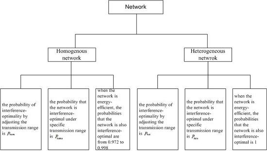
4.1. Homogenous Node Deployment Probability Analysis

In homogenous WSNs, all the nodes have the same transmission ranges and the transmission ranges are circular.

Theorem 1.

In homogenous WSNs, the relationship between the overlapping coverage area s and the node distance d is approximately linear, which is $s=\mathsf{\pi }{r}^2-1.93r\cdot d$.

Proof.

As shown in Figure 5, the distance between node u and node v is d; the intersection points of the overlapping coverage area are A and B, respectively. Thus, the acreage of the shade area in Figure 5 can be calculated as:

$$s=2\cdot r^2\cdot (\arccos \frac{d}{2r})-d\cdot \sqrt{r^2-\frac{d^2}{4}}$$

(5)

where r is the transmission radius. Based on the Taylor Formula, the Taylor Expansion of Equation (5) is:

$$s_t=\mathsf{\pi }{r}^2-(r+1)\cdot d+o[(\frac{d}{2r}{)}^3]$$

(6)

where $\frac{d}{2r}\in (0,\frac{1}{2})$; since $o[(\frac{d}{2r}{)}^3]$ is small, then the relationship between the overlapping coverage area s and the node distance d is approximately linear according to Equation (6). For simplifying the calculation of Equation (5), we assume:

$$f=\mathsf{\pi }{r}^2-kr\cdot d$$

(7)

Additionally, we define the difference between s and f is:

$$\begin{array}{ll}y& =s-f\\ & =2\cdot r^2\cdot (\arccos \frac{d}{2r})-d\cdot \sqrt{r^2-\frac{d^2}{4}}-(\mathsf{\pi }{r}^2-kr\cdot d)\end{array},$$

(8)

The variance of the difference y is:

$$D(y)=E(y^2)-{[E(y)]}^2$$

(9)

$$D(y){|}_k^{\prime }=E(y^2){|}_k^{\prime }-{[E(y)]}^2{|}_k^{\prime }$$

(10)

where $E(\cdot )$ is the operator of mathematical expectation. In Equation (10), when $0<k<1.93$, $D(y)|{}_k^{\prime }<0$; when $k>1.93$, $D(y)|{}_k^{\prime }>0$; therefore, when $k=1.93$, the $D(y)$ can get the minimum value. This conclusion also can be found in Figure 6.

Therefore, the linear function of two nodes’ overlapping coverage area can be expressed as:

$$f=\mathsf{\pi }{r}^2-1.93r\cdot d,$$

(11)

For investigating the evaluation error between s and f, we define the evaluation error as:

$$e=\frac{y}{s}=1-\frac{f}{s},$$

(12)

Figure 6 and Figure 7 show the variance of y and the evaluation error between s and f, respectively. In this simulation, r = 100.

From Figure 6, we can conclude that with the increasing of k, the variance will obtain the minimum value when k is 1.93, which is consistent with the theoretical analysis in Equation (10). Figure 7 indicates that when the value of k is 1.93, the evaluation error between s and f is smaller than 0.015, which is small enough to be ignored. In addition, when $k=1.93$, the variance and evaluation error are minimum simultaneously. Therefore, the Equation (11) can be used to evaluate two nodes’ overlapping coverage area in homogenous WSNs.

The simulation results of Equations (5) and (11) are shown in Figure 8. In Figure 8, the Equations (5) and (11) are fitted with small evaluation error. This indicates that in homogenous WSNs, the relationship between the overlapping coverage area and the node distance is linear.

Even this conclusion is obtained under the assumption that r = 100; however, when the value of r changes, we can get the same conclusion as Equation (11).

Theorem 2.

In homogeneous networks, the probability of interference-optimality by adjusting the transmission range is:

$$\begin{array}{ll}{p}_{\mathrm{hom}}& ={\displaystyle {\int }_0^{0.85r}p(r-r_1\le d_1\le 0.19\cdot \sqrt{r_1{}^2+27.67r^2}-r)}+{\displaystyle {\int }_{0.85r}^{r}p(r-r_1\le d_1\le 2.63(\frac{r^2}{r_1}-r_1))}\\ & ={\displaystyle {\int }_0^{0.85r}(e^{-\mathsf{\pi }\mathsf{\rho }(r-r_1{)}^2}-e^{-\mathsf{\pi }\mathsf{\rho }{(0.19\cdot \sqrt{r_1{}^2+27.67r^2}-r)}^2}})d{r}_1+{\displaystyle {\int }_{0.85r}^r(e^{-\mathsf{\pi }\mathsf{\rho }{(r-r_1)}^2}-e^{-\mathsf{\pi }\mathsf{\rho }{(\frac{2.63}{r_1}{r}^2-2.63r_1)}^2}})d{r}_1\end{array}$$

Proof. 

Considering the conclusion of Theorem 1, the coverage area before transmission range adjustment (shown in Figure 2a) is:

$$\begin{array}{ll}{s}_r& =\mathsf{\pi }{r}^2+\mathsf{\pi }{r}^2-(\mathsf{\pi }{r}^2-1.93rd)\\ & =\mathsf{\pi }{r}^2+1.93rd\end{array},$$

(13)

where r is the original transmission range, d is the distance between two nodes.

When the transmission ranges are reduced, the network topology is shown in Figure 2b. In Figure 2b, the distance (u, n) is d₀ and the distance (n, v) is d₁. Therefore, the coverage area of node n, node u, and node v can be calculated as:

$$\begin{array}{ll}{s}_{r_1}& =\mathsf{\pi }{r}_1{}^2+\mathsf{\pi }{r}_1{}^2-(\mathsf{\pi }{r}_1{}^2-1.93r_1{d}_0)+\pi r_1{}^2-(\mathsf{\pi }{r}_1{}^2-1.93r_1{d}_1)\\ & =\mathsf{\pi }{r}_1{}^2+1.93r_1(d_0+d_1)\end{array},$$

(14)

In (14), there are three parts: (1) $\mathsf{\pi }{r}_1{}^2$ is the area of circle u; (2) $\mathsf{\pi }{r}_1{}^2-(\mathsf{\pi }{r}_1{}^2-1.93r_1{d}_0)$ is the area of circle n after removing the overlapping area between circle u and circle n; (3) $\mathsf{\pi }{r}_1{}^2-(\mathsf{\pi }{r}_1{}^2-1.93r_1{d}_1)$ is the area of circle v after removing the overlapping area between circle n and circle v. Moreover, in Equation (14), since d₀ and d₁ are all variables, for simplifying the calculation, we assume that the distance d₀ is equal to the transmission range of node u, i.e., $r_1=d_0$. This assumption is reasonable. Since the distance equal to the transmission range means the node which is farthest from the source node will be chosen as the relay node. For instance, as shown in Figure 4, when the node u sends data packet to node v, the source node u will choose node n which is in the boundary of the coverage area as the relay node; therefore, the transmission range is equal to the distance (u, n), i.e., the distance (u, n) is the maximum value among all the neighbors’ distances. Thus, when the transmission ranges are reduced, the coverage area can be rewritten as:

$$\begin{array}{ll}{s}_{r_1}& =\mathsf{\pi }{r}_1{}^2+\mathsf{\pi }{r}_1{}^2-(\mathsf{\pi }{r}_1{}^2-1.93r_1{}^2)+\mathsf{\pi }{r}_1{}^2-(\mathsf{\pi }{r}_1{}^2-1.93r_1{d}_1)\\ & =5.07r_1{}^2+1.93r_1{d}_1\end{array}$$

(15)

Additionally, in Equation (15), $r_1$ is the transmission range after being reduced and equal to the maximum value between distance (u, n) and distance (n, v). For instance, as shown in Figure 4, distance (n, v) is smaller than distance (u, n) and equal to d₁; so $r_1$ is equal to distance (u, n) and larger than d₁ (the situation that r₁ is smaller than d₁ will be investigated following). In this scenario, the transmission ranges of node u, node v, and node n are all the same and equal to $r_1$.

Based on the principle of linear programming, the boundary condition of this issue is $\mathsf{\rho }{s}_r=\mathsf{\rho }{s}_{r_1}$ (as shown in Section 3, the interference can be calculated by Equation (4), the boundary condition means the interference before transmission range adjustment is equal to the interference that after the transmission range adjustment), which can be expressed as:

$$d_1=2.63\cdot (\frac{r^2}{r_1}-r_1),$$

(16)

In addition, when the transmission ranges are reduced, for guaranteeing the network connection, r₁ and d₁ should satisfy the constraints as follows:

$$\{\begin{array}{l}0<r_1<r\\ 0<d_1<r\\ r_1>d_1\\ r_1+d_1>r\end{array},$$

(17)

In the calculation of the coverage area, we assume that $r_1$ is larger than d₁, i.e., $0<d_1<r_1$, so based on Equations (16) and (17), the feasible region when $0<d_1<r_1$ is the triangle DBC in Figure 9.

In the coverage area calculation, $r_1=d_0$ and the role of d₀ and d₁ are equal in Equation (14), i.e., d₀ and d₁ can be replaced by each other in Equation (14). Therefore, when distance (u, n) is smaller than the distance (n, v), i.e., $r_1<d_1$, the feasible region should be symmetrical to DBC based on line $d_1=r_1$. So, according to Equation (16), when $r_1$ is smaller than d₁, the boundary will be $d_1=0.19(\sqrt{r_1{}^2+27.67r^2}-r)$ (this boundary condition can be obtained by variable swapping between r₁ and d₁ in Equation (16)). In this situation, the feasible region is DBA in Figure 9. The whole feasible region is triangle ABC which can be found in the shade area of Figure 9.

In Figure 9, when $r_1$ and d₁ equal to the values in shade area, the network interference will decrease; otherwise, the interference will increase. In addition, the coordinate of B is (0.85r, 0.85r), so when $0<r_1<0.85r$, the value range of d₁ is ($r-r_1$, $0.19(\sqrt{r_1{}^2+27.67r^2}-r)$); when $0.85r<r_1<r$, the value range is ($r-r_1$, $2.63(\frac{r^2}{r_1}-r_1)$), where AC represents the line $r-r_1$ in Figure 9.

In [27], the authors have proved that if the nodes are uniformly distributed in the network, the probability density function (PDF) of the neighbor distance is Rayleigh Distribution:

$$f(d)=2\mathsf{\pi }\mathsf{\rho }d\cdot e^{-\mathsf{\pi }\mathsf{\rho }{d}^2} (d>0),$$

(18)

where d is the distance between two nodes, and $\mathsf{\rho }$ is the node density. Thus the probability that the neighbors’ distances are larger than $d_1$ and smaller than $d_2$ can be calculated as:

$$P(d_1\le r\le d_2)={\displaystyle {\int }_{d_1}^{d_2}f(x)dx}=e^{-\mathsf{\pi }\mathsf{\rho }{d}_1^2}-e^{-\mathsf{\pi }\mathsf{\rho }{d}_2^2},$$

(19)

As shown in Figure 9, the probability that the distance between two nodes, $r_1$, can be calculated by Equation (18). The probability that d₁ satisfies the constraints shown in Figure 9 can be calculated by Equation (19). Then the probability that the network is interference-optimal by adjusting the transmission range is:

$$\begin{array}{ll}{p}_{\mathrm{hom}}& ={\displaystyle {\int }_0^{0.85r}p(r-r_1\le d_1\le 0.19\cdot \sqrt{r_1{}^2+27.67r^2}-r)}+{\displaystyle {\int }_{0.85r}^{r}p(r-r_1\le d_1\le 2.63(\frac{r^2}{r_1}-r_1))}\\ & ={\displaystyle {\int }_0^{0.85r}(e^{-\mathsf{\pi }\mathsf{\rho }{(r-r_1)}^2}-e^{-\mathsf{\pi }\mathsf{\rho }{(0.19\cdot \sqrt{r_1{}^2+27.67r^2}-r)}^2}})d{r}_1+{\displaystyle {\int }_{0.85r}^r(e^{-\mathsf{\pi }\mathsf{\rho }{(r-r_1)}^2}-e^{-\mathsf{\pi }\mathsf{\rho }{(\frac{2.63}{r_1}{r}^2-2.63r_1)}^2}})d{r}_1\end{array},$$

(20)

The Equation (20) indicates that the probability relates to both the original transmission range r and the node density $\mathsf{\rho }$. The properties of this probability under different r and $\mathsf{\rho }$ will be investigated in the simulation part in detail.

However, the probability shown in Equation (20) is just a general probability. This probability measures the possibility that, for the different original transmission ranges, when the transmission ranges are reduced, there exist optimal solutions which can guarantee low network interference. However, the probability of interference-optimality under specific transmission range is different with that in Equation (20).

Theorem 3.

In homogeneous networks, the probability that the network is interference-optimal under specific transmission range can be calculated by:

$$P_{\mathrm{homs}}=\{\begin{array}{l}{\displaystyle {\int }_{r-r_1}^{0.19(\sqrt{r_1{}^2+27.67r^2}-r)}2\mathsf{\pi }\mathsf{\rho }{d}_1\cdot e^{-\mathsf{\pi }\mathsf{\rho }{d}_1{}^2}}d{d}_1, (0<r_1<0.85r)\\ {\displaystyle {\int }_{r-r_1}^{2.63(\frac{r^2}{r_1}-r_1)}2\mathsf{\pi }\mathsf{\rho }{d}_1\cdot e^{-\mathsf{\pi }\mathsf{\rho }{d}_1{}^2}d{d}_1}, (0.85r<r_1<r)\end{array}$$

Proof. 

As shown in Figure 9, when, $0<r_1<0.85r$, the value range of d₁ is ($r-r_1$, $0.19(\sqrt{r_1{}^2+27.67r^2}-r)$); when $0.85r<r_1<r$, the value range is ($r-r_1$, $2.63(\frac{r^2}{r_1}-r_1)$). According to the probability density function (PDF) (18), the integral of the PDF shown in (18) on the value range of d₁ represents the probability of interference-optimality under specific transmission range, which can be calculated as:

$$P_{homs}=\{\begin{array}{l}{\displaystyle {\int }_{r-r_1}^{0.19(\sqrt{r_1{}^2+27.67r^2}-r)}2\mathsf{\pi }\mathsf{\rho }{d}_1\cdot e^{-\mathsf{\pi }\mathsf{\rho }{d}_1{}^2}}d{d}_1, (0<r_1<0.85r)\\ {\displaystyle {\int }_{r-r_1}^{2.63(\frac{r^2}{r_1}-r_1)}2\mathsf{\pi }\mathsf{\rho }{d}_1\cdot e^{-\mathsf{\pi }\mathsf{\rho }{d}_1{}^2}d{d}_1}, (0.85r<r_1<r)\end{array},$$

(21)

This probability means that under specific transmission range, the possibility that the network is interference-optimal.

Corollary 1.

In homogeneous networks, when the transmission range is 0.85r, the probability that the network is interference-optimal will get the maximum value.

Proof.

To Equation (21), when $0<r_1<0.85r$, $P_{\mathrm{homs}}^{\prime }>0$; when $0.85r<r_1<r$, $P_{\mathrm{homs}}^{\prime }<0$. Therefore, if $d_1=0.85r$, $P_{\mathrm{homs}}$ can get the maximum value, i.e., if the transmission range is 0.85r, the probability that the network is interference-optimal will get the maximum value.

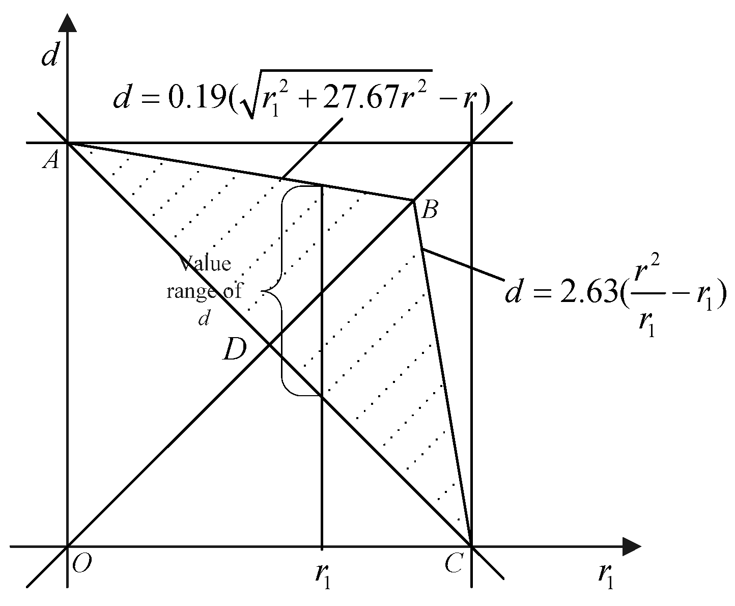
4.2. Heterogeneous Node Deployment Probability Analysis

In Section 4.1, the obtained asymptotic results are based on the assumption that each node has the same transmission range, which is often not the case in practice. In this section, we will analyze the probability of interference-optimality under the assumption that the transmission ranges are different in the network.

As shown in Figure 10, we assume that the transmission range of node u is larger than node v. So there are two different positions of node v: (1) as shown in Figure 10a, the distance between node u and node v is smaller than r and larger than $r/2$, i.e., $r/2\le d\le r$. In this scenario, node v falls into the coverage area of node u and the overlapping area is part of node v’s coverage area. (2) As shown in Figure 10b, the distance between node u and node v is smaller than $r/2$, i.e., $0\le d\le r/2$. In this scenario, the whole coverage area of node v will be included by node u. The coverage area calculation will be different in these two scenarios.

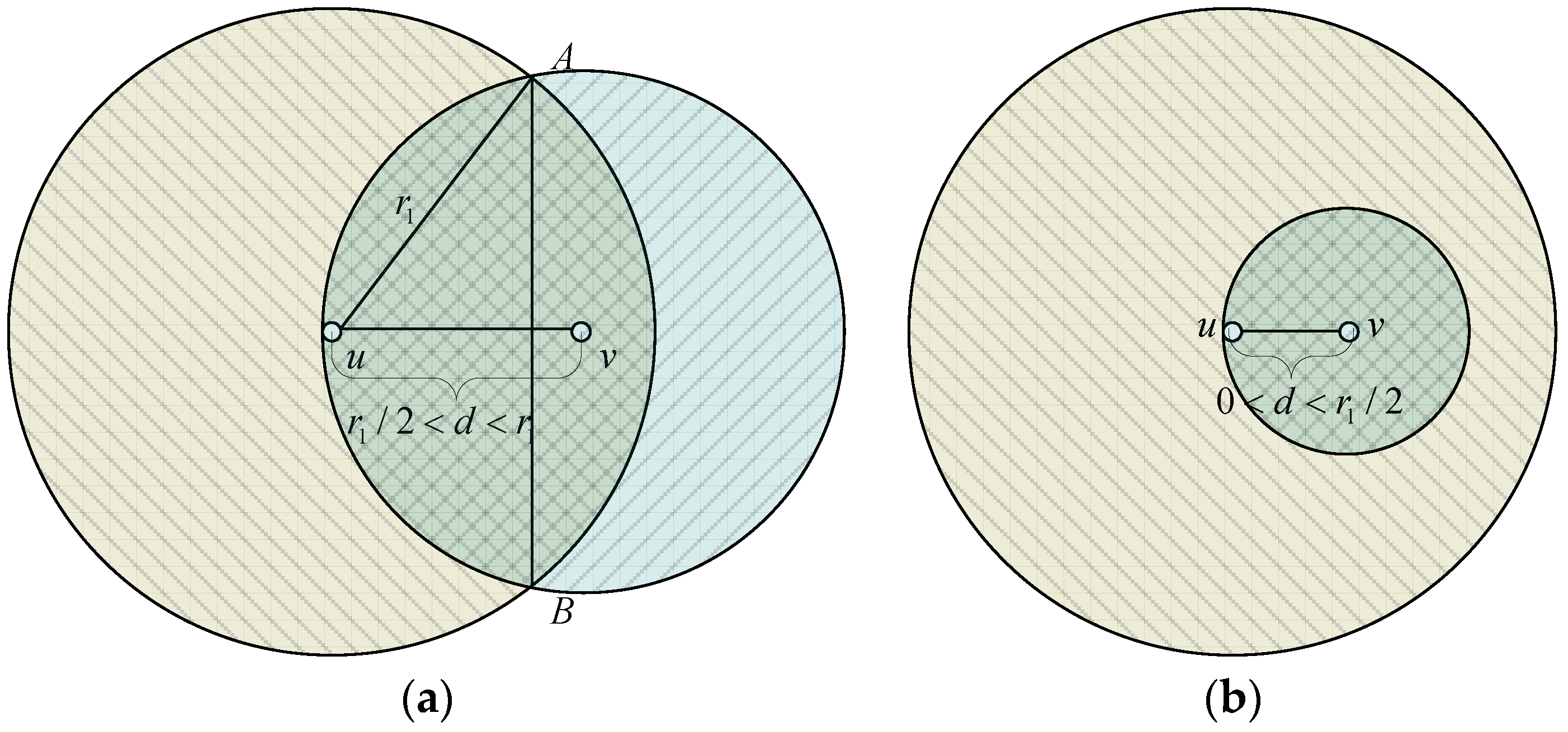
4.2.1. The Node Distance is $r/2\le d\le r$

Theorem 4.

In the heterogeneous WSNs, if the distance between node u and node v is smaller than r and larger than $r/2$, the relationship between the overlapping coverage area s and the node distance d is approximately $s=-1.57\cdot d^2+3.23\cdot rd-0.44\cdot r^2$.

Proof. 

As shown in Figure 10a, when the transmission ranges of two nodes are different, the overlapping coverage area can be calculated as:

$$s=r^2\arccos \frac{r}{2d}+2d^2\arcsin \frac{r}{2d}-r\sqrt{d^2-{\left(\frac{r}{2}\right)}^2},$$

(22)

where r is the transmission range of node u, and d is the distance between two nodes. Based on the Taylor Formula, the Taylor Expansion of Equation (22) is:

$$s_t=\frac{\mathsf{\pi }}{2}{d}^2-\frac{d}{2r}+o[{(\frac{d}{2r})}^3],$$

(23)

where $\frac{d}{2r}\in (\frac{1}{4},\frac{1}{2})$; since the $o[{(\frac{d}{2r})}^3]$ is small, so the relationship between the overlapping coverage area s and the node distance d is approximately quadratic. For simplifying the calculation of Equation (22), we assume:

$$f=a{d}^2+brd+c{r}^2,$$

(24)

Additionally, we define the difference between s and f as:

$$\begin{array}{ll}y& =s-f\\ & =r^2\arccos \frac{r}{2d}+2d^2\arcsin \frac{r}{2d}-r\sqrt{d^2-{\left(\frac{r}{2}\right)}^2}-(a{d}^2+brd+c{r}^2)\end{array},$$

(25)

The variance of the difference y is:

$$D(y)=E(y^2)-{[E(y)]}^2,$$

(26)

$$D(y)|{}_a^{\prime }=E(y^2)|{}_a^{\prime }-{[E(y)]}^2|{}_a^{\prime },$$

(27)

In Equation (27), according to the values ($r/2$, $s_1$) and ($r$, $s_2$) (which can be got from Equation (22)), we can confirm the relationship between a, b and c. The values of s₁ and s₂ are:

$$\{\begin{array}{l}{s}_1=\mathsf{\pi }{d}^2\\ s_2=(\frac{\mathsf{\pi }}{3}+\frac{\sqrt{3}}{2})r^2+\frac{\mathsf{\pi }}{3}{d}^2\end{array},$$

(28)

In Equation (27), when $-\infty <a<-1.57$, $D(y)|{}_a^{\prime }<0$; when $-1.57<a<\infty$, $D(y)|{}_a^{\prime }>0$. Therefore, when $a=-1.57$, the variance of y is minimum. This is also can be found in Figure 11. Thus, Equation (24) can be rewritten as:

$$f=-1.57\cdot d^2+3.23\cdot rd-0.44\cdot r^2,$$

(29)

For investigating the evaluation error between s and f, we define the evaluation error is:

$$e=\frac{y}{s}=1-\frac{f}{s},$$

(30)

The evaluation error between s and f is shown in Figure 12. In Figure 12, we can conclude that the maximum evaluation error between s and f is only 0.025 and the mean absolute value is only 0.0139. This means that the error between s and f can be ignored during the calculation of the overlapping coverage area in heterogeneous networks, i.e., the Equation (29) can be used to calculate the overlapping coverage area approximately. The results of s and f are shown in Figure 13. In Figure 13, the curve of s and f can be fitted in small error. Thus, in the calculation of the overlapping coverage area in heterogeneous WSNs, the Equation (22) can approximately be replaced by the quadratic function.

Based on Theorem 1, the coverage area before adjusting the transmission range is:

$$\begin{array}{ll}{s}_r& =2\mathsf{\pi }{r}^2-(\mathsf{\pi }{r}^2-1.93r^2)\\ & =5.07r^2\end{array},$$

(31)

As shown in Figure 4, based on Theorem 4, the coverage area after adjusting the transmission ranges is:

$$\begin{array}{ll}{s}_{r_1}=\mathsf{\pi }{r}_1{}^2& +\mathsf{\pi }{d}_0^2-(3.23r_1{d}_0-1.57r_1{}^2-0.44d_0^2)\\ & +\mathsf{\pi }{d}_1^2-(3.23d_0{d}_1-1.57d_1^2-0.44d_0^2)\end{array},$$

(32)

In Equation (32), there are three parts: (1) $\mathsf{\pi }{r}_1{}^2$ is the area of circle u; (2) $\mathsf{\pi }{d}_0^2-(3.23r_1{d}_0-1.57r_1{}^2-0.44d_0^2)$ is the area of circle n after removing the overlapping area between circle u and circle n; (3) $\mathsf{\pi }{d}_1^2-(3.23d_0{d}_1-1.57d_1^2-0.44d_0^2)$ is the area of circle v after removing the overlapping area between circle n and circle v. In Equation (32), since d₀ and d₁ are all variables, for simplifying the calculation, we assume that the distance d₀ is equal to the transmission range of node u, i.e., $r_1=d_0$. This assumption is reasonable. Since the distance equal to the transmission range means that the node which is farthest from the source node will be chosen as the relay node. For instance, as shown in Figure 4, when the node u sends data packet to node v, then the node n which is in the boundary of the coverage area will be chosen the relay node; therefore, the transmission range of node u is equal to distance (u, n), i.e., the distance (u, n) is the maximum value among all the neighbors’ distances. Thus, when the transmission ranges are changed, the coverage area can be rewritten as:

$$\begin{array}{l}{s}_{r_1}=\mathsf{\pi }{r}_1{}^2+\mathsf{\pi }{r}_1{}^2-(3.23r_1{}^2-1.57r_1{}^2-0.44r_1{}^2)\\ +\mathsf{\pi }{d}_1^2-(3.23r_1{d}_1-1.57d_1^2-0.44r_1{}^2)\\ =4.62r_1{}^2-3.23r_1{d}_1+4.71d_1^2\end{array},$$

(33)

Similar to the analysis in Section 4.1, the boundary condition is $\mathsf{\rho }{s}_r=\mathsf{\rho }{s}_{r_1}$, which can be expressed as:

$$d_1=0.343r_1+\sqrt{r^2-r_1{}^2},$$

(34)

The transmission range $r_1$ and node distance d₁ should satisfy the constraints shown in Equation (17). In addition, in Equation (33), $r_1$ is the transmission range after adjustment and equal to the maximum value between distance (u, n) and distance (n, v). For instance, as shown in Figure 4, the distance (u, n) is larger than the distance (n, v), so $r_1$ is equal to distance (u, n) and larger than d₁ (the situation that r₁ is smaller than d₁ will be investigated following). Moreover, in this scenario, we assume $r_1/2\le d_1\le r_1$, so the constraints are shown as follows:

$$\{\begin{array}{l}0<r_1<r\\ 0<d_1<r\\ r_1/2<d_1<r_1\\ r_1+d_1>r\end{array},$$

(35)

In Figure 14, the area of constraint $r_1/2\le d_1\le r_1$ in Inequation (35) is between the line OF and OA; the line OF represents $d_1=r_1/2$ and the line OA represents $d_1=r_1$. Therefore, the feasible region when $d_1<r_1$ is KHBA in Figure 14. As discussed in Section 4.1, the role of $r1$ and d₁ are equal in Equations (33) and (34). So when distance (n, v) is larger than distance (u, n), the feasible region should be symmetrical with KHBA based on line $d_1=r_1$ (line OA), which is IKEA in Figure 14. According to Equation (34), when $d_1>r_1$, the transmission range equals to d₁, then the constraint $r_1/2\le d_1\le r_1$ in Inequation (35) will be $d_1/2\le r_1\le d_1$, which is between line OD and line OA; moreover, according to Equation (34), the boundary condition is $d_1=0.445\cdot \sqrt{4.5r^2-4r_1{}^2}+0.31r_1$ for feasible region IKEA in Figure 14. Thus, the whole feasible region in this scenario is EIHB which is shown in Figure 14.

The coordinates of the points in Figure 14 are shown in

Table 2. The coordinates of the points in Figure 14.

Points	A	B	C	D	E	F	G
Coordinate	(0.84r, 0.84r)	(0.99r, 0.495r)	(r, 0.343r)	(r, 0.5r)	(0.495r, 0.99r)	(0.5r, r)	(0.343r, r)

.

4.2.2. The Node Distance is $0\le d\le r/2$

As shown in Figure 10b, when the transmission range of node v is smaller than $r/2$, the whole coverage area of node v will be included by node u; so the overlapping coverage area is $\mathsf{\pi }{d}^2$, which is also the quadratic function. According to Figure 4, in this scenario, when the transmission ranges are reduced, the probability of interference-optimality is 1. Similar to the analysis in the first part of this section, the feasible regions are IFY and HDX in Figure 14.

As shown in Figure 14 and Table 1, the coordinate of point B is $(0.99r,0.495r)$, the coordinates of point D are $(r,0.5r)$, and the coordinates of point C are $(r,0.343r)$. Thus, the areas of HBX and HDX are similar, which means that we can use HBX to represent HDX to simplify the probability calculation in heterogeneous networks. The relationship between IFY and IEY is similar to that between HBX and HDX.

Theorem 5.

In heterogeneous networks, the probability of interference-optimality by adjusting the transmission range is:

$$\begin{array}{l}{p}_{\mathrm{het}}={\displaystyle {\int }_{0.343r}^{0.84r}(}{e}^{-\mathsf{\pi }\mathsf{\rho }{(r-r_1)}^2}-e^{-\mathsf{\pi }\mathsf{\rho }{(0.445\cdot \sqrt{4.5r^2-4r_1{}^2}+0.31r_1)}^2})d{r}_1 +{\displaystyle {\int }_{0.84r}^r(e^{-\mathsf{\pi }\mathsf{\rho }{(r-r_1)}^2}-e^{-\mathsf{\pi }\mathsf{\rho }{(0.343r_1+\sqrt{r^2-r_1{}^2})}^2}})d{r}_1\\ +{\displaystyle {\int }_0^{0.343r}(e^{-\mathsf{\pi }\mathsf{\rho }{(r-r_1)}^2}-e^{-\mathsf{\pi }\mathsf{\rho }{r}^2}})d{r}_1\end{array}$$

Proof.

In Section 4.2, we investigate the constraints of interference-optimality by adjusting the transmission ranges in heterogeneous networks. The whole feasible region is shown in Figure 14 (the shade area). As shown in Figure 14, when $0<r_1<0.343r$, the value range of d₁ is ($r-r_1$, r); when $0.343r<r_1<0.84r$, the value range is ($r-r_1$, $0.445\cdot \sqrt{4.5r^2-4r_1{}^2}+0.31r_1$); when $0.84r<r_1<r$, this will be ($r-r_1$, $0.343r_1+\sqrt{r^2-r_1{}^2}$). Therefore, similarly with the analysis in Section 3 and according to the PDF (19), the probability of interference-optimality by adjusting the transmission range can be calculated as:

$$\begin{array}{l}{p}_{\mathrm{het}}={\displaystyle {\int }_{0.343r}^{0.84r}(}{e}^{-\mathsf{\pi }\mathsf{\rho }{(r-r_1)}^2}-e^{-\mathsf{\pi }\mathsf{\rho }{(0.445\cdot \sqrt{4.5r^2-4r_1{}^2}+0.31r_1)}^2})d{r}_1 +{\displaystyle {\int }_{0.84r}^r(e^{-\mathsf{\pi }\mathsf{\rho }{(r-r_1)}^2}-e^{-\mathsf{\pi }\mathsf{\rho }{(0.343r_1+\sqrt{r^2-r_1{}^2})}^2}})d{r}_1\\ +{\displaystyle {\int }_0^{0.343r}(e^{-\mathsf{\pi }\mathsf{\rho }{(r-r_1)}^2}-e^{-\mathsf{\pi }\mathsf{\rho }{r}^2}})d{r}_1\end{array},$$

(36)

In Equation (36), the probability relates to both the original transmission range and the node density. The properties of this probability under different r and $\mathsf{\rho }$ will be investigated in the simulation part in detail.

Similar to the probability in Equation (20), the probability that is shown in Equation (36) is just a general probability under different original transmission ranges. In terms of a different original transmission range, this probability means the possibility that there exist optimal solutions which can guarantee low network interference if the transmission range is changed. However, the probability of interference-optimality under specific transmission range will be different from that shown in Equation (36).

Theorem 6.

In heterogeneous networks, the probability that the network is interference-optimal under specific transmission range is:

$$P_{\mathrm{hets}}=\{\begin{array}{l}{\displaystyle {\int }_{r-r_1}^{r}2\mathsf{\pi }\mathsf{\rho }{r}_1\cdot e^{-\mathsf{\pi }\mathsf{\rho }{r}_1{}^2}}d{r}_1 , (0<r_1<0.343r)\\ {\displaystyle {\int }_{r-r_1}^{0.445\cdot \sqrt{4.5r^2-4r_1{}^2}+0.31r_1}2\mathsf{\pi }\mathsf{\rho }{r}_1\cdot e^{-\mathsf{\pi }\mathsf{\rho }{r}_1{}^2}}d{r}_1, (0.343r<r_1<0.84r)\\ {\displaystyle {\int }_{r-r_1}^{0.343x+\sqrt{r^2-x^2}}2\mathsf{\pi }\mathsf{\rho }{r}_1\cdot e^{-\mathsf{\pi }\mathsf{\rho }{r}_1{}^2}}d{r}_1, (0.84r<r_1<r)\end{array}.$$

Proof. 

As shown in Figure 9, when $0<r_1<0.343r$, the value range of d₁ is ($r-r_1$, $r$); when $0.84r<r_1<r$, the value range is ($r-r_1$, $0.343r_1+\sqrt{r^2-r_1{}^2}$); when $0.343r<r_1<0.84r$, the value range of d₁ is ($r-r_1$, $0.445\cdot \sqrt{4.5r^2-4r_1{}^2}+0.31r_1$). Therefore, according to the probability density function (PDF) (18), the integral of the PDF shown in (18) on the value range of d₁ represents the probability of interference-optimality under specific transmission range, which can be calculated as:

$$P_{\mathrm{hets}}=\{\begin{array}{l}{\displaystyle {\int }_{r-r_1}^{r}2\mathsf{\pi }\mathsf{\rho }{r}_1\cdot e^{-\mathsf{\pi }\mathsf{\rho }{r}_1{}^2}}d{r}_1 , (0<r_1<0.343r)\\ {\displaystyle {\int }_{r-r_1}^{0.445\cdot \sqrt{4.5r^2-4r_1{}^2}+0.31r_1}2\mathsf{\pi }\mathsf{\rho }{r}_1\cdot e^{-\mathsf{\pi }\mathsf{\rho }{r}_1{}^2}}d{r}_1, (0.343r<r_1<0.84r)\\ {\displaystyle {\int }_{r-r_1}^{0.343x+\sqrt{r^2-x^2}}2\mathsf{\pi }\mathsf{\rho }{r}_1\cdot e^{-\mathsf{\pi }\mathsf{\rho }{r}_1{}^2}}d{r}_1, (0.84r<r_1<r)\end{array},$$

(37)

Corollary 2.

In heterogeneous networks, when the transmission range is 0.84r, the probability of interference-optimal will get the maximum value.

Proof. 

As shown in Equation (37), when $0<r_1<0.84r$, $P_{\mathrm{hets}}^{\prime }>0$; when $0.84r<r_1<r$, $P_{\mathrm{hets}}^{\prime }<0$. So when $r_1=0.84r$, the probability of interference-optimality in the heterogeneous WSNs will get the maximum value.

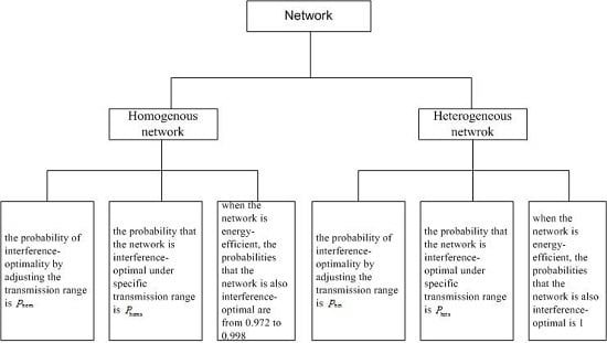
5. The Relationship between Energy-Efficiency and Interference-Optimality

As shown in [24,28,29], the energy required to transmit a data packet from node u to node v relates to the distance between these two nodes, which can be expressed as:

$$P_{uv1}\propto r^{\mathsf{\gamma }},$$

(38)

where r is the Euclidean distance between node u and node v, $\mathsf{\gamma }$ is the distance-power gradient which depends on the characteristics of the communication medium ($2\le \mathsf{\gamma }\le 4$, $\mathsf{\gamma }\ge 2$ for outdoor propagation modes [29]); $P_{uv1}$ is the power needed for the communication link between node u and node v.

As shown in Figure 15, if the transmission ranges of node u and node v are reduced, then node u and node v cannot communicate with each other directly. As a result, node n will be chosen as the relay node, where node n is the neighbor node of both node u and node v. Thus the power needed to transmit packets from node u to node v relates to:

$$P_{uv2}\propto r_1{}^{\mathsf{\gamma }}+r_2{}^{\mathsf{\gamma }},$$

(39)

where $r_1$ is the Euclidean distance between node u and node n, $r_2$ is the Euclidean distance between node n and node v; $P_{uv2}$ is the power needed for the communication link between node u and node v by using the relay node n.

For exploring the probability of reducing the energy consumption by adjusting the transmission range, we define the Energy-efficient Dominating Sets (EDS) as follows:

$$\{\begin{array}{l}{P}_{uv1}\ge P_{uv2}\\ r_1+r_2\ge r\\ 0<r_1\le r\\ 0<r_2\le r\end{array},$$

(40)

The first constraint in Inequation (40) guarantees the energy consumption is smaller to previous values; the second constraint makes sure that the network is still connected after the transmission range adjustment; the third and the fourth constraints guarantee that the transmission ranges of each node are smaller to previous values.

5.1. Homogenous Node Deployment Mode

Theorem 7.

In the homogeneous networks, when the network is energy-efficient, the probabilities that the network is also interference-optimal are from 0.972 to 0.998.

Proof. 

As discussed in Section 4.1, in homogeneous networks, the feasible region of interference-optimality is shown in Figure 9. Considering the Inequations (40) and (17), the feasible region of both energy-efficiency and interference-optimality can be found in Figure 16. The boundary conditions of energy-efficiency and interference-optimality in Figure 16 are shown in Equations (41) and (42), respectively:

$$d_e={(r^{\mathsf{\gamma }}-r_1{}^{\mathsf{\gamma }})}^{\frac{1}{\mathsf{\gamma }}},$$

(41)

$$d_i=\{\begin{array}{l}0.19(\sqrt{r_1{}^2+27.67r^2}-r), (0<r_1<0.85r) \\ 2.63\cdot (\frac{r^2}{r_1}-r_1), (0.85r<r_1<r)\end{array},$$

(42)

Figure 17 illustrates the relationship between energy-efficiency and interference-optimality. From Figure 16 and Figure 17, we can find that with the increasing of the distance-power gradient $\mathsf{\gamma }$, the feasible region of energy-efficiency increases; moreover, the probability that the requirements of interference-optimality and energy-efficiency cannot be satisfied simultaneous increases, too.

The coordinates of E, F and H in Figure 16 are shown in

Table 3. The coordinates of E, F and H.

Coordinates	F	E	H
$\mathsf{\gamma }=2$	(0.94r, 0.36r)	(0.36r, 0.94r)	(0.71r, 0.71r)
$\mathsf{\gamma }=3$	(0.88r, 0.68r)	(0.68r, 0.88r)	(0.79r, 0.79r)
$\mathsf{\gamma }=4$	(0.86r, 0.83r)	(0.83r, 0.86r)	(0.84r, 0.84r)

.

Therefore, as shown in Figure 16, when the network is energy-efficient, the value ranges that the network is not interference-optimal at the same time are the region (AE, $\stackrel{⌢}{AE}$) and region (FC, $\stackrel{⌢}{FC}$). Moreover, these two regions are equal since they are symmetrical to line OB. Therefore, the probabilities can be calculated as:

(1)

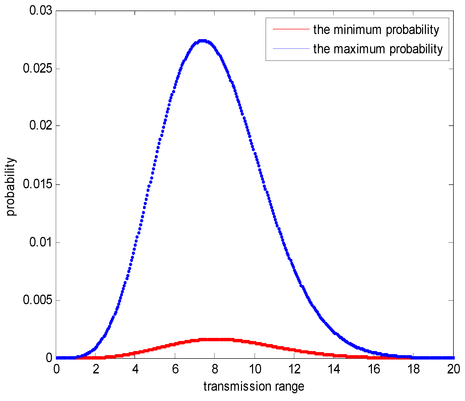
The minimum probability can be calculated when $\mathsf{\gamma }=2$:

$$\begin{array}{cc}\hfill p_{\min }& =2\cdot {\displaystyle {\int }_0^{0.36r}(e^{-\mathsf{\pi }\mathsf{\rho }(r^2-r_1{}^2)}-e^{-\mathsf{\pi }\mathsf{\rho }{(0.19\cdot \sqrt{r_1{}^2+27.67r^2}-r)}^2}})\cdot 2\mathsf{\pi }\mathsf{\rho }{r}_1\cdot e^{-\mathsf{\pi }\mathsf{\rho }{r}_1{}^2}d{r}_1\hfill \\ & =0.002\hfill \end{array},$$

(43)

(2)

The maximum probability can be calculated when $\mathsf{\gamma }=4$:

$$\begin{array}{cc}\hfill p_{\max }& =2\cdot {\displaystyle {\int }_0^{0.83r}(e^{-\mathsf{\pi }\mathsf{\rho }(r^4-r_1{}^4)\frac{1}{2}}-e^{-\mathsf{\pi }\mathsf{\rho }{(0.19\cdot \sqrt{r_1{}^2+27.67r^2}-r)}^2}})\cdot 2\mathsf{\pi }\mathsf{\rho }{r}_1\cdot e^{-\mathsf{\pi }\mathsf{\rho }{r}_1{}^2}d{r}_1\hfill \\ & =0.028\hfill \end{array}$$

(44)

According to Equations (43) and (44), when the network is energy-efficient, the probabilities that the network is also interference-optimal are from 0.972 to 0.998, which are pretty high. So in most cases, we can observe that the energy-efficient network is approximately an interference-optimal network.

5.2. Heterogeneous Node Deployment Mode

Theorem 8.

In the heterogeneous networks, when the network is energy-efficient, the probability that the network is also interference-optimal is approximately 1.

In Section 4.2, when the transmission ranges are different in the network, the feasible regions of interference-optimality and energy-efficiency are shown in Figure 18. Considering Equation (40), the boundaries of energy-efficiency and interference-optimality are shown in Figure 19.

Similar to Figure 17, in Figure 19, when $\mathsf{\gamma }=4$, the feasible region of energy-efficiency is the largest and approximately equal to the feasible region of interference-optimality. The evaluation error can be found in Figure 20. In Figure 20, when $\mathsf{\gamma }=4$, the evaluation error between the feasible region of energy-efficiency and interference-optimality is only $6.5\times {10}^{-4}$, which is small and can be ignored. Therefore, in heterogeneous networks, the probability that the network is energy-efficient and interference-optimal at the same time is approximately equal to 1. Consequently, we can conclude that in heterogeneous WSNs, when the network is energy-efficient, the network is interference-optimal, not vice versa.

According to the conclusions of Section 5.1 and Section 5.2, on one hand, in heterogeneous WSNs, when the network is energy-efficient, the network is also interference-optimal with probability 1; on the other hand, since the transmission ranges are always heterogeneous in practice, we can observe that the energy-efficient network is the interference-optimal network.

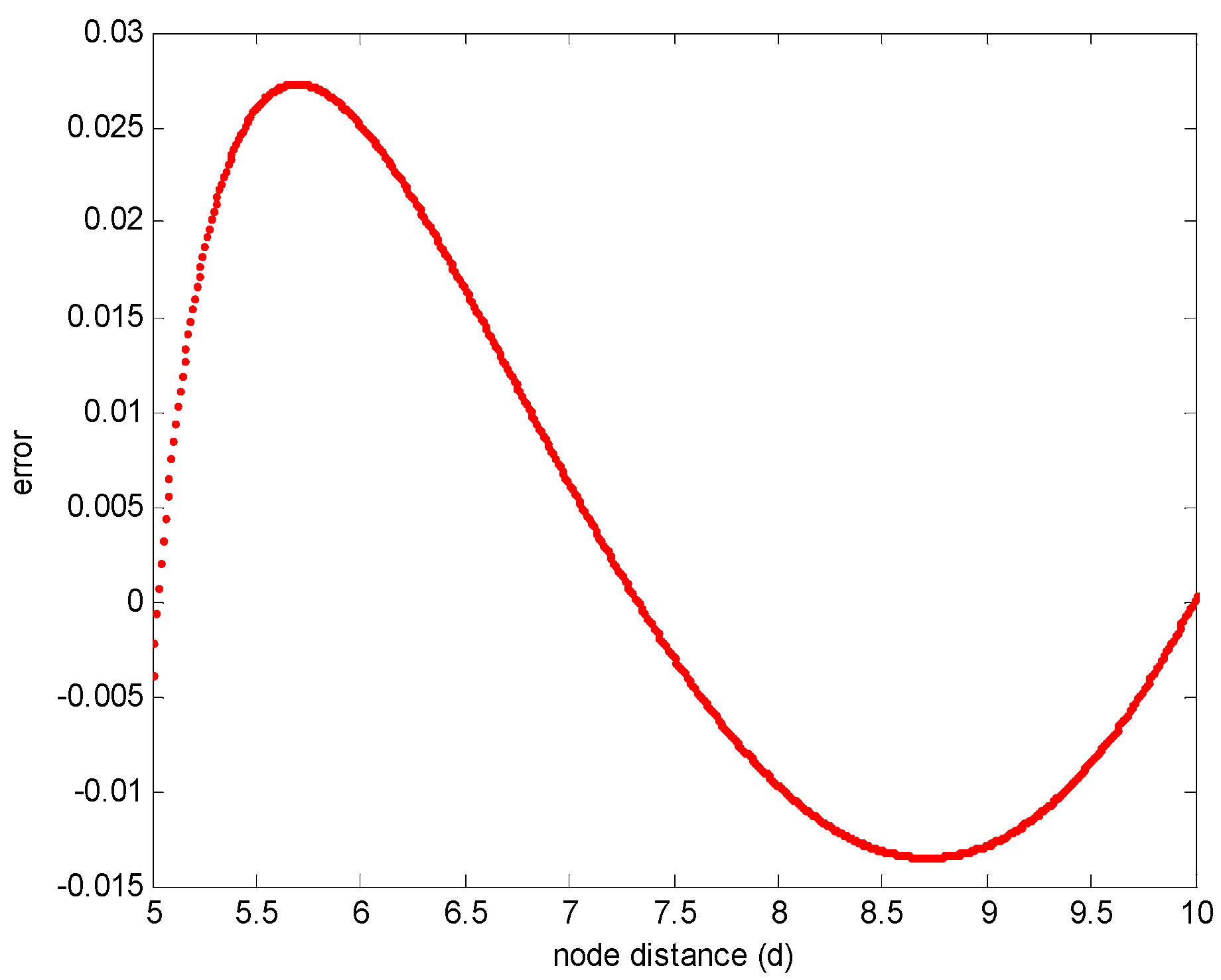
6. Simulation and Discussion

In Section 4 and Section 5, we investigate the probability of interference-optimality by adjusting the transmission range and explore the properties of this probability in detail. In this section, we will evaluate this probability by simulation and compare the simulation results with the theory analysis.

6.1. Probability Analysis in Homogenous Network

The PDF of the neighbor distance (shown in Equation (18)) can be found in Figure 21. The Figure 21 indicates that the distribution of the neighbor node distance is Rayleigh Distribution. In Figure 21, with the increasing of the node density, the maximum probability increases while the maximum neighbor distance decreases. The reason is that when the node density increases, more nodes are deployed in the same area, so the neighbor distances decrease. For instance, in Figure 21, when the node densities are 0.1, 0.01, and 0.005, the maximum neighbor node distances are 5, 15, and 20, respectively. The similar variation trend can be found in the neighbor node distances which have the maximum probabilities.

Equation (17) is the probability of interference-optimality by adjusting the transmission range in homogenous WSNs, which relates to both the original transmission range and the node density. The simulation results under different initial transmission ranges and node densities are shown in Figure 22.

In Figure 22, the node densities vary from 0.005 to 0.1 and the original transmission ranges vary from 0 to 25. With the increasing of the original transmission ranges, the probabilities that the network is interference-optimal increase to 1 when the original transmission ranges are larger than the maximum neighbor distance that is shown in Figure 22. For instance, in Figure 22, when the node density is 0.1, with the increasing of the original transmission range, the probability increases when the transmission range is smaller than 5 and levels off to 1 when the transmission range is larger than 5. The same variation trend can be found when the node densities are 0.01 and 0.005. The trend in Figure 22 is consistent with the simulation results of Figure 21. In Figure 21, when the node density is 0.1, the maximum neighbor distance is 5 (when the probability is equal to 0 in Figure 21); meanwhile, in Figure 22, when the node density is 0.1 and the transmission range is larger than 5, the probability of interference-optimality by adjusting the transmission range levels off to 1. The reason is that under the specific node density, if the original transmission range is larger than the maximum neighbor node distance, then, once the transmission ranges are reduced, the optimal transmission range can be found with probability 1.

Under different node densities, the probabilities of interference-optimality by adjusting the transmission ranges are different. As shown in Figure 22, when the node density increases, the probability increases under the same original transmission range. For instance, when the original transmission range is 10, the probabilities are 0.51, 0.85, and 1 when the node densities are 0.05, 0.01, and 0.1, respectively. In addition, the optimal transmission ranges under different node densities are equal to the maximum neighbor node distances shown in Figure 21.

Figure 23 describes the probability under specific transmission range, in which the original transmission range and node density are fixed to 10 and 0.01, respectively. From Figure 23, we can conclude that the maximum probability is approximately 0.83 when the transmission range is 0.85r. Therefore, the maximum probability is 0.83 and the optimal transmission range is 0.85r. This conclusion means that when the transmission range is 0.85r, the probability of interference-optimality is the highest. This conclusion is consistent with the theoretical analysis in Section 4.1.

6.2. Probability Analysis in Heterogeneous Networks

Similar to the homogenous WSNs, the probabilities in heterogeneous WSNs are shown in Figure 24 and Figure 25.

Figure 24 and Figure 25 indicate that the properties of the probability in heterogeneous networks are similar to that in homogeneous networks. The differences are the values of the probability and the optimal transmission range. In Figure 22 and Figure 24, the minimum original transmission ranges (which the probability is 1) are consistent with the maximum neighbor distances that are shown in Figure 21. The differences between Figure 22 and Figure 24 are due to the different boundary conditions in heterogeneous networks and homogeneous networks. These can be found in Equations (16) and (34), Figure 9 and Figure 14. Since the feasible region in heterogeneous networks is larger than that in homogeneous networks, the probability in heterogeneous networks is also larger than that in homogeneous networks under the same network conditions. For instance, in Figure 24, when the node density is 0.01 and the original transmission range is 10, the probability is 0.897; while in Figure 23, this probability is 0.862, which is smaller than that in Figure 24. The same conclusion can be obtained when the node density and the original transmission range are changed.

Similar to the homogenous network, in Figure 25, with the increasing of transmission range, the probability under specific transmission range increases from 0 to 0.82 and reaches the maximum value when the transmission range is 0.84r; the probability decreases when the transmission range is larger than 0.84r. Therefore, the maximum probability is 0.82 and the optimal transmission range is 0.84r in the homogenous network. This conclusion is interesting, since the maximum probability and the optimal transmission range are similar in homogenous WSNs and heterogeneous WSNs.

6.3. The Relationship between Interference-Optimality and Energy Efficiency

In this section, we will evaluate the relationship between interference-optimality and energy-efficiency. According to the conclusions of Section 5.2, in heterogeneous networks, when the network is energy-efficient, the network is also interference-optimal with probability 1. The evaluation errors shown in Figure 20 are tiny. Therefore, in this part, we mainly investigate the relationship between the interference-optimality and the energy-efficiency in homogeneous networks, which has been analyzed in Section 5.1.

According to Equations (43) and (44), the maximum and minimum probabilities that the network cannot meet interference-optimality and energy-efficiency simultaneously can be found in Figure 26. In Figure 26, the node density is 0.01.

From Figure 26, we can conclude that when the node density is 0.01, if the network is energy-efficient, the maximum and minimum probabilities that the network is not interference-optimal are only 0.028 and 0.0016, respectively. Therefore, the evaluation errors are small enough to be ignored. Based on the conclusions of Section 5.1 and Section 5.2, we can conclude that when the network is energy-efficient, the network is also interference-optimal both in the homogeneous and heterogeneous WSNs.

7. Conclusions

In this paper, we investigate the probability of interference-optimality by adjusting the transmission range. First, we prove that the interference issues can be abstracted as the issues of node’s coverage. The relationships between the coverage area and the distance between two nodes are approximately linear and quadratic in homogeneous network and heterogeneous network, respectively. The probability of interference-optimality by adjusting the transmission range relates to the node density $\mathsf{\rho }$ and the original transmission range r, which can be found in Figure 22 and Figure 24. Based on the probability functions that we proposed, we find the optimal transmission range which has the highest probability of interference-optimality. The optimal transmission ranges in homogeneous networks and heterogeneous networks are 0.85r and 0.84r, respectively. In addition, we also prove that when the network is energy-efficient, the probability that the network is also interference-optimal is approximately 1. This conclusion means that the energy-efficient network is also the interference-optimal network at the same time.

The conclusions of this paper can be used in the probability analysis of WSNs in the future.

References

1. Yick, J.; Mukherjee, B.; Ghosal, D. Wireless sensor networks survey. Comput. Netw. 2008, 52, 2292–2330. [Google Scholar] [CrossRef]
2. Akyildiz, I.F.; Su, W.; Sankarasubramaniam, Y.; Cayirci, E. Wireless sensor networkss: A survey. Comput. Netw. 2002, 38, 393–422. [Google Scholar] [CrossRef]
3. Rawat, P.; Singh, K.D.; Chaouchhi, H.; Bonnin, J.M. Wireless sensor networkss: A survey on recent development and potential synergies. J. Supercomput. 2013, 68, 1–48. [Google Scholar] [CrossRef]
4. Huang, Y.; Martinez, J.F.; Sendra, J.; Lopez, L. Resilient wireless sensor networks using topology control: A review. Sensors 2015, 15, 24735–24770. [Google Scholar] [CrossRef] [PubMed]
5. Burkhart, M.; von Rickenbach, P.; Wattenhofer, R.; Zollinger, A. Does topology control reduce interference? In Proceedings of the 5th ACM International Symposium on Mobile Ad Hoc Networking and Computing (MobiHoc’04), Tokyo, Japan, 24–26 May 2004; pp. 9–19.
6. Von Rickenbach, P.; Wattenhofer, R.; Zollinger, A. Algorithm models of interference in wireless ad hoc and sensor networks. IEEE/ACM Trans. Netw. 2009, 17, 172–185. [Google Scholar] [CrossRef]
7. Aziz, A.A.; Sekercioglu, Y.A.; Fitzpatrick, P.; Ivanovich, M. A Survey on distributed topology control techniques for extending the lifetime of battery power wireless sensor networks. IEEE Commun. Surv. Tutor. 2013, 15, 121–144. [Google Scholar] [CrossRef]
8. Li, M.; Li, Z.; Vasilakos, A.V. A survey on topology control in wireless sensor networkss: Taxonomy, comparative study, and open issues. Proc. IEEE Brows. J. Mag. 2013, 101, 2538–2557. [Google Scholar] [CrossRef]
9. Johansson, T.; Carr-Motyckova, L. Reducing interference in ad hoc networks through topology control. In Proceedings of the 2005 Joint Workshop on Foundations of Mobile Computing (DIALM-POMC’05), Cologne, Germany, 2 September 2005; pp. 17–23.
10. Moaveni-Nejad, K.; Li, X. Low interference topology control for wireless ad hoc networks. Ad Hoc Sens. Wirel. Netw. 2005, 1, 41–64. [Google Scholar]
11. Chiwewe, T.M.; Hancke, G.P. A distributed topology control technique for low interference and energy efficiency in wireless sensor networks. IEEE Trans. Ind. Inform. 2012, 8, 11–19. [Google Scholar] [CrossRef]
12. Zhang, X.M.; Zhang, Y.; Yan, F.; Vasilakos, A.V. Interference Based topology control algorithm for delay constrained mobile ad hoc networks. IEEE Trans. Mob. Comput. 2015, 14, 742–754. [Google Scholar] [CrossRef]
13. Sun, G.; Zhao, L.; Chen, Z.; Qiao, G. Effective link interference model in topology control of wireless ad hoc and sensor network. J. Netw. Comput. Appl. 2015, 52, 69–78. [Google Scholar] [CrossRef]
14. Von Rickenbach, P.; Wattenhofer, R.; Zollinger, A. A robust interference model for wireless ad hoc networks. In Proceedings of the 19th IEEE International Parallel and Distributed Processing Symposium (IPDP’05), Denver, CO, USA, 4–8 April 2005; pp. 1–8.
15. Lou, T.; Tan, H.; Wang, Y.; Lau, F.C.M. Minimizing average interference through topology control. In Proceedings of the 7th International Symposium on Algorithms for Sensor Systems, Wireless Ad Hoc Networks and Autonomous Mobile Entities (ALGOSENSORS 2011), Saarbrucken, Germany, 8–9 September 2011; pp. 115–129.
16. Huang, J.; Liu, S.; Xing, G.; Zhang, H.; Wang, J.; Huang, L. Accuracy-aware interference modeling and measurement in wireless sensor networks. In Proceedings of the 31th International Conference on Distributed Computing Systems, Minneapolos, MN, USA, 20–24 June 2011; pp. 172–181.
17. De Heide, F.M.A.; Schindelhauer, C.; Volbert, K.; Grunewald, M. Energy, congestion and dilation in ratio networks. In Proceedings of the Fourteenth Annual ACM Symposium on Parallel Algorithms and Architectures (SPAA’02), Winnipeg, MB, Canada, 11–13 August 2002; pp. 230–237.
18. Halldorsson, M.M.; Tokuyama, T. Minimizing interference of a wireless ad hoc network in a plane. Theor. Comput. Sci. 2008, 402, 29–42. [Google Scholar] [CrossRef]
19. Cardieri, P. Modeling Interference in Wireless Ad Hoc Network. IEEE Commun. Surv. Tutor. 2007, 12, 551–572. [Google Scholar] [CrossRef]
20. Blough, D.M.; Leoncini, M.; Resta, G.; Santi, P. Topology control with better radio models: Implications for energy and multi-hop interference. Perform. Eval. 2007, 64, 379–398. [Google Scholar] [CrossRef]
21. Liu, S.; Xing, G.; Zhang, H.; Wang, J. Passive interference measurement in wireless sensor networks. In Proceedings of the 18th IEEE International Conference on Network Protocols (ICNP), Kyoto, Japan, 5–8 October 2010; pp. 52–61.
22. Hermans, F.; Rensferl, O.; Voigt, T.; Ngai, E.; Norden, L.; Gunningverg, P. Sonic: Classifying interference in 802.15.4 sensor networks. In Proceedings of the 12th International Conference on Information Processing in Sensor Networks (IPSN’13), Philadelphia, PA, USA, 8–11 April 2013; pp. 55–66.
23. Cong, Y.; Zhou, X.; Kennedy, R.A. Interference Prediction in Mobile Ad Hoc Networks with a General Mobility Model. IEEE Trans. Wirel. Commun. 2015, 14, 4277–4290. [Google Scholar] [CrossRef]
24. Huang, Y.; Martinez, J.F.; Sendra, J.; Lopez, L. The influence of communication range on connectivity for resilient wireless sensor networks using a probabilistic approach. Int. J. Distrib. Sens. Netw. 2013. [Google Scholar] [CrossRef]
25. Bettstetter, C. On the minimum node degree and connectivity of a wireless multihop network. In Proceedings of the 3rd ACM International Symposium on Mobile Ad Hoc Networking and Computing (MobiHoc’02), Lausanne, Switzerland, 9–11 June 2002; pp. 80–91.
26. Mekikis, V.; Antonopoulos, A.; Kartsakli, E.; Lalos, A.; Alonso, L.; Verikoukis, C. Information Exchange in Randomly Deployed Dense WSNs with Wireless Energy Harvesting Capabilities. IEEE Trans. Wirel. Commun. 2016, 15, 3008–3018. [Google Scholar] [CrossRef]
27. Cressie, N.A.C. Statistics for Spatial Data; Wiley-Interscience Publication: New York, NY, USA, 1990; pp. 577–725. [Google Scholar]
28. Zhu, Y.; Huang, M.; Chen, S.; Wang, Y. Energy-efficient topology control in cooperative ad hoc network. IEEE Trans. Parallel Distrib. Syst. 2012, 23, 1480–1491. [Google Scholar] [CrossRef]
29. Rappaport, T.S. Wireless Communication: Principles and Practive; Prentice-Hall: Englewood Cliffs, NJ, USA, 1996; pp. 69–122, 139–196. [Google Scholar]
Figure 1. Different network models: (a) k nearest neighbor model; (b) disc model; (c) Erdos-Renyi random graph.
Applsci 06 00396 g001
Figure 2. Different Disc Models: (a) Homogeneous Disc Model; (b) Heterogeneous Disc Model.
Applsci 06 00396 g002
Figure 3. Interference before adjusting the transmission range.
Applsci 06 00396 g003
Figure 4. Interference after adjusting the transmission range.
Applsci 06 00396 g004
Figure 5. The overlapping coverage area in homogeneous networks.
Applsci 06 00396 g005
Figure 6. The variance of the difference between s and f under different value of k.
Applsci 06 00396 g006
Figure 7. The evaluation error between s and f.
Applsci 06 00396 g007
Figure 8. The fitting results of Equations (5) and (11).
Applsci 06 00396 g008
Figure 9. The feasible region in homogeneous networks.
Applsci 06 00396 g009
Figure 10. Different node positions in heterogeneous networks: (a) r / 2 d r ; (b) 0 d r / 2 .
Applsci 06 00396 g010
Figure 11. The variance of difference between s and f under different value of a.
Applsci 06 00396 g011
Figure 12. The evaluation error between s and f.
Applsci 06 00396 g012
Figure 13. The fitting results of Equations (22) and (29).
Applsci 06 00396 g013
Figure 14. The feasible region in Heterogeneous networks.
Applsci 06 00396 g014
Figure 15. Transmission range adjustment in energy-efficiency analysis.
Applsci 06 00396 g015
Figure 16. The feasible region of energy-efficiency and interference-optimality in homogeneous networks.
Applsci 06 00396 g016
Figure 17. The boundary of energy-efficiency and interference-optimality in homogeneous networks.
Applsci 06 00396 g017
Figure 18. The feasible region of energy-efficiency and interference-optimality in heterogeneous networks.
Applsci 06 00396 g018
Figure 19. The boundary of energy-efficiency and interference-optimality in heterogeneous networks.
Applsci 06 00396 g019
Figure 20. The error between the boundaries of energy-efficiency and interference-optimality.
Applsci 06 00396 g020
Figure 21. The probability density function of (17).
Applsci 06 00396 g021
Figure 22. The probability under different node density and original transmission range in homogeneous networks.
Applsci 06 00396 g022
Figure 23. The probability under different transmission range in homogeneous networks.
Applsci 06 00396 g023
Figure 24. The probability under different node density and original transmission range in heterogeneous networks.
Applsci 06 00396 g024
Figure 25. The probability under different transmission range in heterogeneous networks.
Applsci 06 00396 g025
Figure 26. The probability that the network cannot meet the requirements of interference-optimality and energy-efficiency.
Applsci 06 00396 g026