
Sparse Representation-Based SAR Image Target Classification on the 10-Class MSTAR Data Set


Abstract
:
1. Introduction
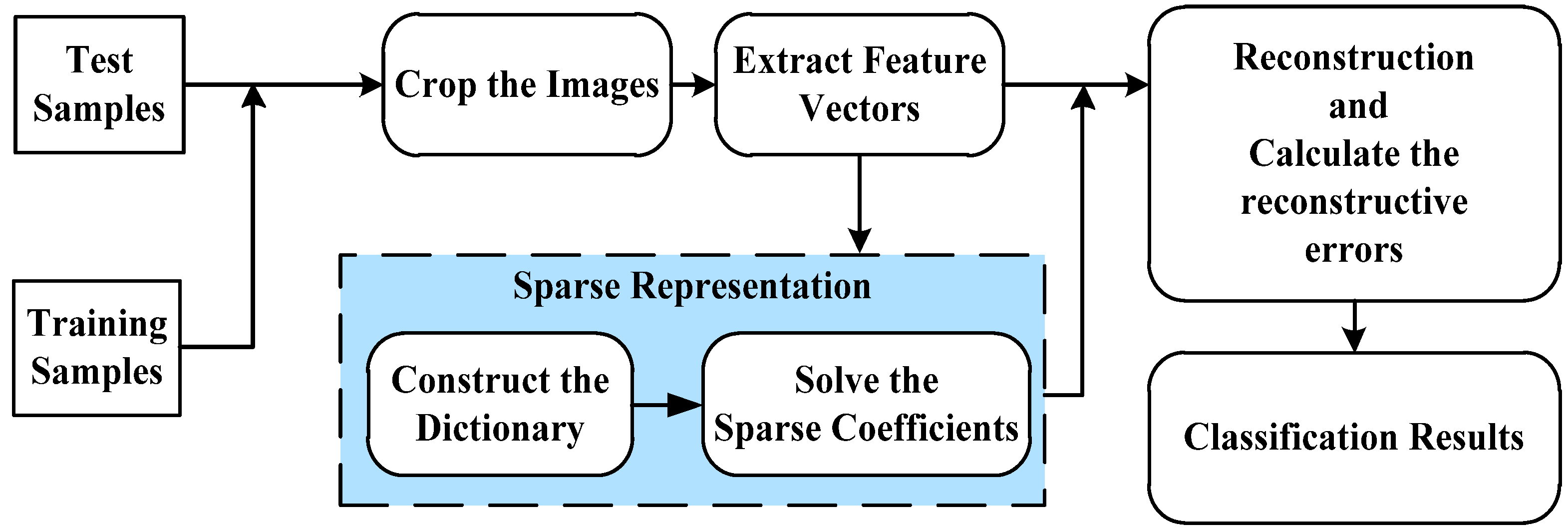
2. Sparse Representation-Based Classification
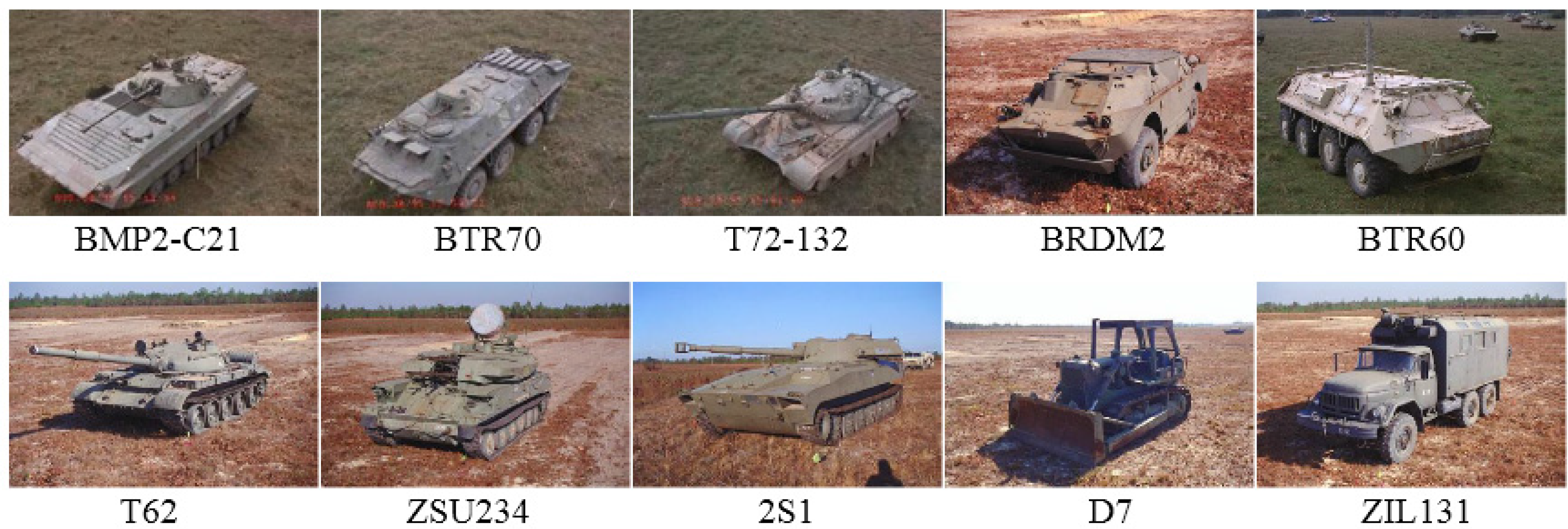
3. Classification on the 10-Class MSTAR Targets


4. Experiment Results

| Targets | BMP2 | BTR70 | T72 | BTR60 | 2S1 | BRDM2 | D7 | T62 | ZIL131 | ZSU234 |
|---|---|---|---|---|---|---|---|---|---|---|
| 17° | 233 | 233 | 232 | 256 | 299 | 298 | 299 | 299 | 299 | 299 |
| 15° | 587 | 196 | 582 | 195 | 274 | 274 | 274 | 273 | 274 | 274 |
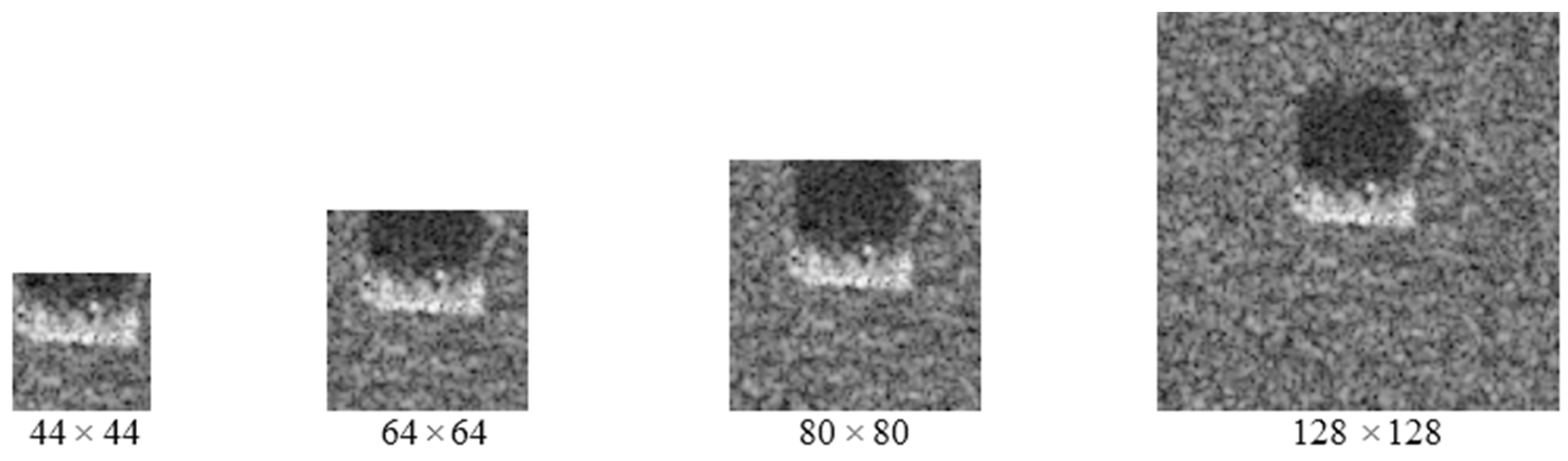
| Patch | 44 × 44 Pixel | 64 × 64 Pixel | 80 × 80 Pixel |
|---|---|---|---|
| Accuracy | 34.1% | 64.3% | 75.1% |
4.1. Recognition Accuracy of Two Classifiers
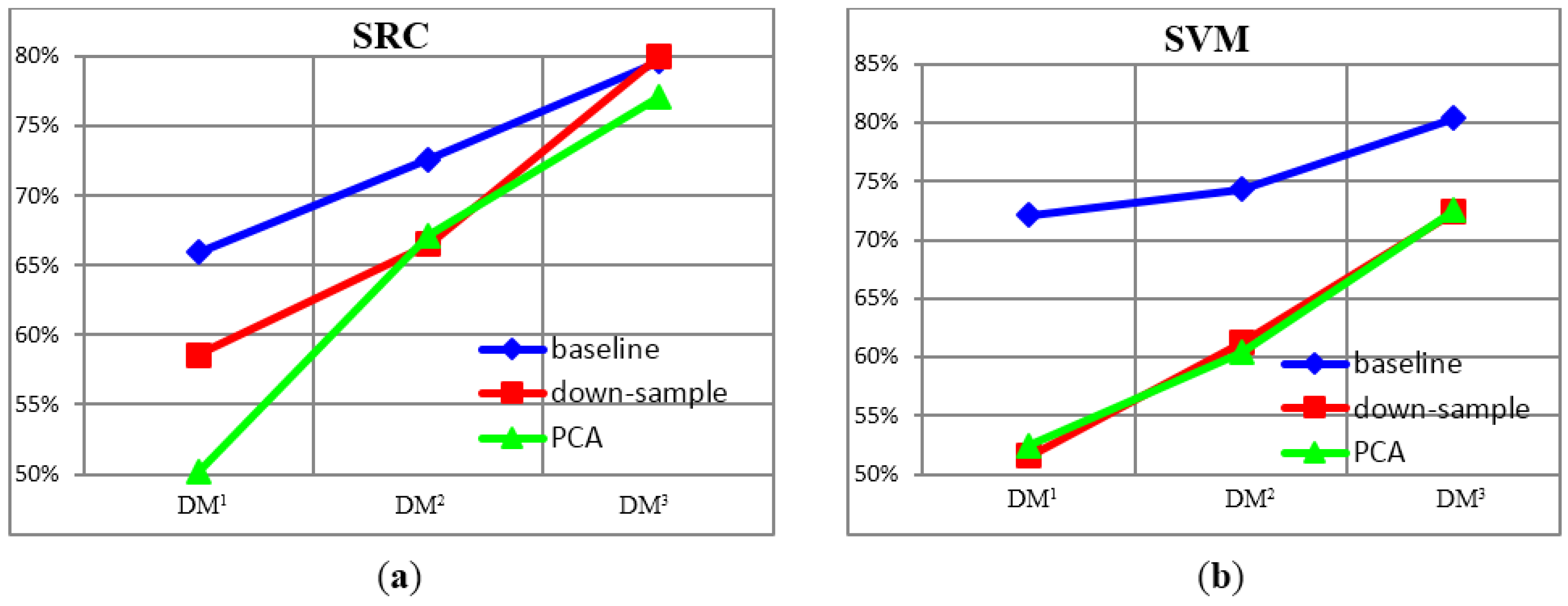
4.1.1. Comparison between Conventional Features and Unconventional Features

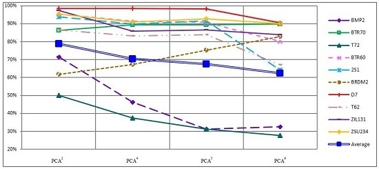
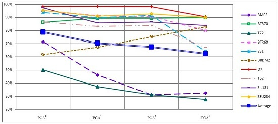
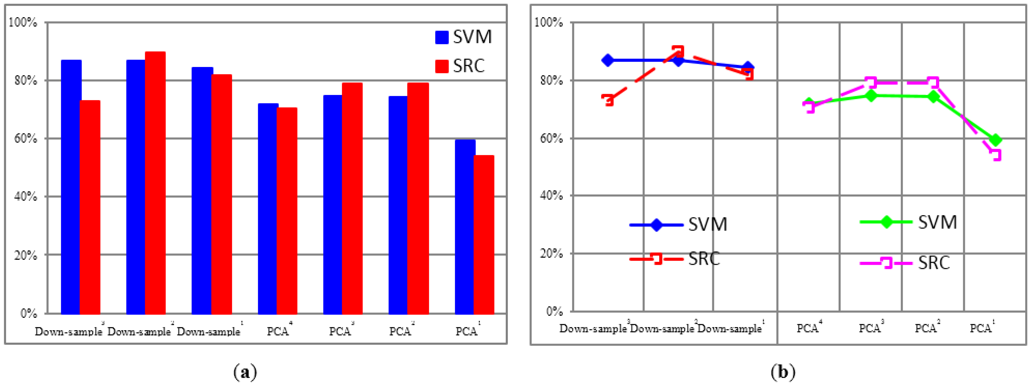
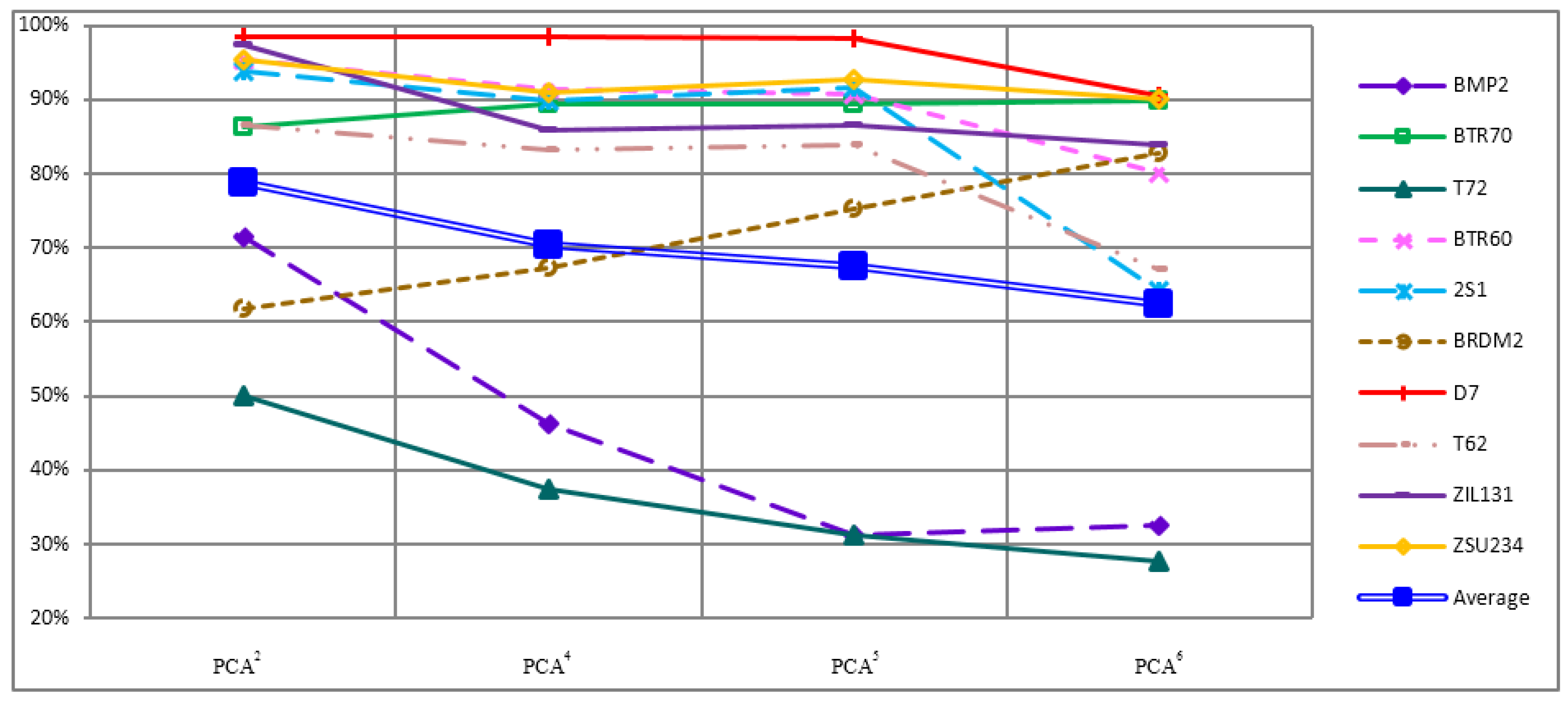
4.1.2. Recognition Accuracy under Unconventional Feature Spaces
| Features | Down-Sample3 | Down-Sample2 | Down-Sample1 | PCA4 | PCA3 | PCA2 | PCA1 |
|---|---|---|---|---|---|---|---|
| SVM | 86.79% | 86.73% | 84.39% | 71.84% | 74.71% | 74.40% | 59.19% |
| SRC | 72.93% | 89.76% | 81.83% | 70.34% | 78.89% | 78.86% | 54.04% |

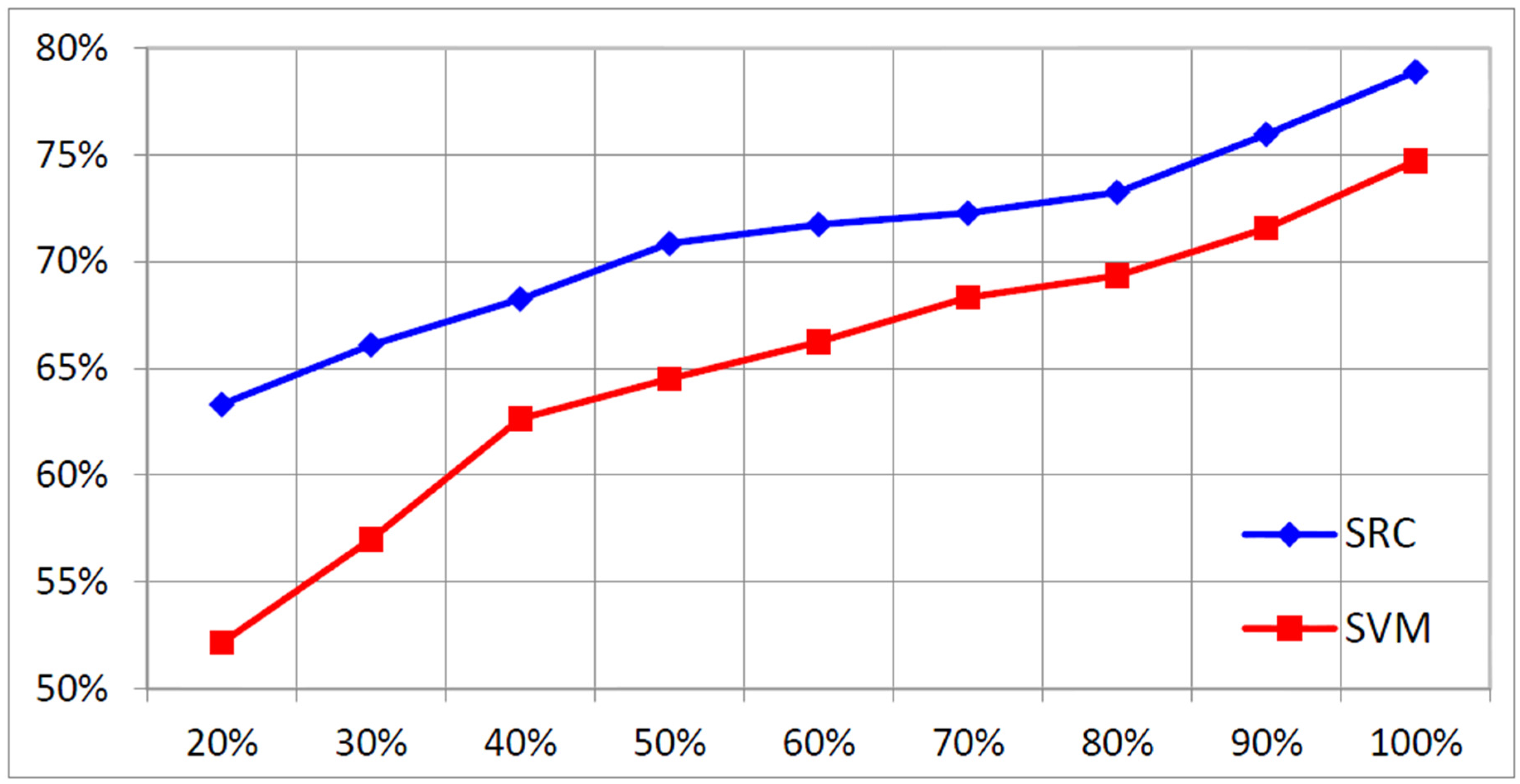
4.2. Recognition Accuracy under Incomplete Training Samples
4.3. Recognition Rate of Each Object
| SVM | Features | Targets | BMP2 | BTR70 | T72 | BTR60 | 2S1 | BRDM2 | D7 | T62 | ZIL131 | ZSU234 | SRC | Features | Targets | BMP2 | BTR70 | T72 | BTR60 | 2S1 | BRDM2 | D7 | T62 | ZIL131 | ZSU234 |
| a | BMP2 | 83.6 | 1.5 | 8.5 | 2.0 | 4.1 | 0.0 | 0.0 | 0.2 | 0.0 | 0.0 | a | BMP2 | 79.4 | 4.1 | 10.2 | 3.6 | 0.3 | 0.7 | 0.5 | 0.3 | 0.0 | 0.9 | ||
| BTR70 | 2.0 | 93.9 | 0.0 | 0.0 | 4.1 | 0.0 | 0.0 | 0.0 | 0.0 | 0.0 | BTR70 | 0.0 | 98.5 | 0.5 | 1.0 | 0.0 | 0.0 | 0.0 | 0.0 | 0.0 | 0.0 | ||||
| T72 | 9.6 | 0.7 | 73.0 | 0.0 | 5.5 | 0.0 | 0.0 | 10.3 | 0.9 | 0.0 | T72 | 8.1 | 5.2 | 77.8 | 7.6 | 0.0 | 1.0 | 0.0 | 0.2 | 0.0 | 0.2 | ||||
| BTR60 | 1.0 | 1.5 | 0.0 | 95.4 | 0.0 | 0.5 | 0.0 | 0.5 | 0.0 | 1.0 | BTR60 | 0.0 | 0.0 | 0.0 | 100.0 | 0.0 | 0.0 | 0.0 | 0.0 | 0.0 | 0.0 | ||||
| 2S1 | 0.4 | 0.0 | 1.5 | 1.1 | 92.3 | 0.7 | 0.0 | 3.3 | 0.7 | 0.0 | 2S1 | 0.4 | 0.0 | 1.1 | 0.7 | 95.6 | 2.2 | 0.0 | 0.0 | 0.0 | 0.0 | ||||
| BRDM2 | 1.1 | 2.2 | 0.4 | 4.4 | 3.3 | 85.0 | 0.0 | 0.0 | 3.3 | 0.4 | BRDM2 | 0.4 | 2.9 | 5.5 | 3.3 | 1.1 | 86.5 | 0.4 | 0.0 | 0.0 | 0.0 | ||||
| D7 | 0.0 | 0.0 | 0.0 | 0.0 | 0.4 | 0.4 | 97.4 | 0.0 | 0.0 | 1.8 | D7 | 0.0 | 0.0 | 0.7 | 0.0 | 0.0 | 0.0 | 99.3 | 0.0 | 0.0 | 0.0 | ||||
| T62 | 0.4 | 0.0 | 0.7 | 0.0 | 3.3 | 0.0 | 0.7 | 79.5 | 9.5 | 5.9 | T62 | 0.7 | 0.0 | 0.7 | 1.1 | 0.0 | 0.7 | 0.4 | 95.6 | 0.0 | 0.7 | ||||
| ZIL131 | 0.0 | 0.0 | 0.0 | 0.0 | 0.4 | 0.0 | 0.4 | 2.2 | 96.4 | 0.7 | ZIL131 | 0.0 | 0.0 | 0.0 | 2.2 | 0.4 | 0.0 | 0.0 | 0.4 | 97.1 | 0.0 | ||||
| ZSU234 | 0.0 | 0.0 | 0.0 | 0.0 | 0.0 | 0.0 | 4.4 | 0.4 | 1.1 | 94.2 | ZSU234 | 0.0 | 0.0 | 0.0 | 0.4 | 0.4 | 0.0 | 0.7 | 0.0 | 0.0 | 98.5 | ||||
| b | BMP2 | 71.7 | 8.2 | 8.3 | 4.3 | 2.6 | 2.6 | 0.2 | 0.9 | 0.3 | 1.0 | b | BMP2 | 46.2 | 1.7 | 0.9 | 0.3 | 7.3 | 0.3 | 16.0 | 10.6 | 4.1 | 12.6 | ||
| BTR70 | 1.5 | 91.3 | 0.0 | 4.6 | 1.5 | 1.0 | 0.0 | 0.0 | 0.0 | 0.0 | BTR70 | 0.0 | 89.3 | 0.0 | 0.0 | 2.6 | 0.0 | 2.0 | 3.6 | 0.5 | 2.0 | ||||
| T72 | 12.2 | 6.5 | 49.0 | 2.1 | 13.4 | 2.7 | 0.7 | 7.9 | 5.2 | 0.3 | T72 | 0.0 | 1.5 | 37.5 | 0.2 | 10.1 | 0.0 | 14.9 | 17.0 | 7.6 | 11.2 | ||||
| BTR60 | 1.0 | 5.6 | 1.0 | 85.1 | 2.6 | 2.6 | 0.0 | 0.5 | 0.0 | 1.5 | BTR60 | 0.0 | 0.0 | 0.0 | 91.3 | 2.1 | 0.0 | 4.1 | 0.5 | 0.0 | 2.1 | ||||
| 2S1 | 1.8 | 8.0 | 4.4 | 1.5 | 74.8 | 0.4 | 0.0 | 4.7 | 3.3 | 1.1 | 2S1 | 0.0 | 0.0 | 0.0 | 0.0 | 89.8 | 0.0 | 3.3 | 3.3 | 0.7 | 2.9 | ||||
| BRDM2 | 4.7 | 1.5 | 1.5 | 3.6 | 3.6 | 73.7 | 0.0 | 4.7 | 4.0 | 2.6 | BRDM2 | 0.0 | 0.0 | 0.0 | 0.4 | 4.0 | 67.2 | 7.3 | 7.3 | 6.6 | 7.3 | ||||
| D7 | 0.0 | 0.0 | 0.4 | 0.4 | 0.0 | 1.5 | 89.8 | 1.5 | 1.1 | 5.5 | D7 | 0.0 | 0.0 | 0.0 | 0.0 | 0.4 | 0.0 | 98.5 | 0.7 | 0.4 | 0.0 | ||||
| T62 | 1.5 | 2.9 | 4.4 | 0.4 | 12.8 | 1.8 | 1.5 | 63.7 | 6.2 | 4.8 | T62 | 0.0 | 0.0 | 0.4 | 0.4 | 3.3 | 0.0 | 7.3 | 83.2 | 3.3 | 2.2 | ||||
| ZIL131 | 0.4 | 0.0 | 0.4 | 1.1 | 10.6 | 0.0 | 1.5 | 5.1 | 79.2 | 1.8 | ZIL131 | 0.4 | 0.0 | 0.0 | 0.4 | 2.6 | 0.0 | 7.7 | 2.6 | 85.8 | 0.7 | ||||
| ZSU234 | 0.7 | 0.4 | 1.1 | 0.4 | 0.4 | 0.7 | 9.5 | 6.6 | 5.1 | 75.2 | ZSU234 | 0.0 | 0.0 | 0.0 | 0.0 | 0.4 | 0.0 | 7.3 | 1.5 | 0.0 | 90.9 | ||||
| c | BMP2 | 75.6 | 5.8 | 9.4 | 3.1 | 2.6 | 2.7 | 0.0 | 0.3 | 0.0 | 0.5 | c | BMP2 | 71.6 | 2.9 | 1.5 | 0.5 | 6.0 | 0.7 | 2.7 | 5.8 | 1.2 | 7.2 | ||
| BTR70 | 2.0 | 86.7 | 2.6 | 3.1 | 5.6 | 0.0 | 0.0 | 0.0 | 0.0 | 0.0 | BTR70 | 0.0 | 86.2 | 0.5 | 1.5 | 4.6 | 0.0 | 1.5 | 1.0 | 2.0 | 2.6 | ||||
| T72 | 11.3 | 4.1 | 62.0 | 0.7 | 11.0 | 4.1 | 0.3 | 4.1 | 2.2 | 0.0 | T72 | 0.3 | 2.1 | 50.0 | 1.0 | 5.7 | 0.2 | 6.9 | 22.0 | 4.8 | 7.0 | ||||
| BTR60 | 2.6 | 5.6 | 1.0 | 84.6 | 1.0 | 3.6 | 0.0 | 1.0 | 0.0 | 0.5 | BTR60 | 0.0 | 1.0 | 1.0 | 95.4 | 0.0 | 0.5 | 1.0 | 1.0 | 0.0 | 0.0 | ||||
| 2S1 | 3.6 | 4.7 | 7.3 | 1.5 | 70.4 | 3.6 | 0.0 | 4.7 | 3.6 | 0.4 | 2S1 | 0.0 | 0.0 | 0.7 | 0.0 | 93.8 | 0.0 | 0.4 | 3.3 | 0.4 | 1.5 | ||||
| BRDM2 | 2.2 | 4.4 | 5.8 | 5.5 | 8.4 | 63.9 | 0.0 | 2.9 | 5.5 | 1.5 | BRDM2 | 0.0 | 0.4 | 0.0 | 2.9 | 2.6 | 61.7 | 5.1 | 7.3 | 11.7 | 8.4 | ||||
| D7 | 0.0 | 0.0 | 0.0 | 0.7 | 0.4 | 0.0 | 96.0 | 0.4 | 0.7 | 1.8 | D7 | 0.0 | 0.0 | 0.0 | 0.4 | 0.0 | 0.0 | 98.5 | 0.0 | 1.1 | 0.0 | ||||
| T62 | 0.7 | 1.1 | 1.8 | 0.4 | 13.2 | 7.0 | 0.7 | 61.9 | 8.4 | 4.8 | T62 | 0.0 | 0.0 | 1.1 | 0.4 | 1.8 | 0.0 | 3.3 | 86.4 | 5.5 | 1.5 | ||||
| ZIL131 | 0.4 | 0.4 | 1.5 | 0.0 | 1.8 | 1.8 | 0.7 | 4.0 | 89.1 | 0.4 | ZIL131 | 0.0 | 0.0 | 0.0 | 0.0 | 0.7 | 0.0 | 0.7 | 0.7 | 97.4 | 0.4 | ||||
| ZSU234 | 2.6 | 0.0 | 0.0 | 2.6 | 0.0 | 7.3 | 6.9 | 5.1 | 2.9 | 72.6 | ZSU234 | 0.0 | 0.0 | 0.0 | 0.0 | 0.0 | 0.0 | 2.2 | 2.2 | 0.4 | 95.3 |
5. Conclusions
Acknowledgments
Author Contributions
Conflicts of Interest
References
- Thiagarajan, J.; Ramamurthy, K.; Knee, P.P.; Spanias, A.; Berisha, V. Sparse representation for automatic target classification in SAR images. In Proceedings of Communications, Control and Signal Processing (ISCCSP), 2010 4th International Symposium on, Limassol, Cyprus, 3–5 March 2010.
- Owirka, G.J.; Verbout, S.M.; Novak, L.M. Template-based SAR ATR performance using different image enhancement techniques. Proc. SPIE 1999, 3721, 302–319. [Google Scholar]
- Patnaik, R.; Casasent, D.P. MSTAR object classification and confuser and clutter rejection using minace filters. In Proceedings of Automatic Target Recognition XVI, Orlando, FL, USA, 17 April 2006.
- Marinelli, M.P.; Kaplan, L.M.; Nasrabadi, N.M. SAR ATR using a modified learning vector quantization algorithm. In Proceedings of the SPIE Algorithms for Synthetic Aperture Radar Imagery VI, Orlando, FL, USA, 5 April 1999.
- Yuan, C.; Casasent, D. A new SVM for distorted SAR object classification. In Proceedings of the SPIE Conference on Optical Pattern Recognition XVI, Orlando, FL, USA, 28 March 2005.
- Huang, J.B.; Yang, M.H. Fast sparse representation with prototype. In Proceedings of the IEEE Computer Society Conference on Computer Vision and Pattern Recognition (CVPR 2010), San Francisco, CA, USA, 13–18 June 2010; pp. 3618–3625.
- Shin, Y.; Lee, S.; Woo, S.; Lee, H. Performance increase by using an EEG sparse representation based classification method. In Proceedings of the IEEE International Conference on Consumer Electronics, Las Vegas, NV, USA, 2013; pp. 201–203.
- Huang, X.; Wang, P.; Zhang, B.; Qiao, H. SAR target recognition using block-sparse representation. In Proceedings of the International Conference on Mechatronic Sciences, Electric Engineering and Computer, Shengyang, China, 20–22 December 2013; pp. 1332–1336.
- Dong, G.; Wang, N.; Kuang, G. Sparse representation of monogenic signal: With application to target recognition in SAR images. IEEE Signal Process. Lett. 2014, 21, 952–956. [Google Scholar]
- Xing, X.; Ji, K.; Zou, H.; Sun, J. SAR vehicle recognition based on sparse representation along with aspect angle. Sci. World J. 2014, 2014. [Google Scholar] [CrossRef] [PubMed]
- Pati, Y.C.; Rezaiifar, R.; Krishnaprasad, P.S. Orthogonal matching pursuit: Recursive function approximation with applications to wavelet decomposition. In Proceedings of the Conference Record of The Twenty-Seventh Asilomar Conference on Signals, Systems, and Computers, Pacific Grove, CA, USA, 1–3 November 1993; pp. 40–44.
- Chen, S.; Billings, S.; Luo, W. Orthogonal least squares methods and their application to non-linear system identification. Int. J. Control 1989, 50, 1873–1896. [Google Scholar] [CrossRef]
- Candes, E.; Romberg, J. l1-magic: Recovery of sparse signals via convex programming. California Institute of Technology. 2005. Available online: http://thesis-text-naim-mansour.googlecode.com/svn/trunk/ThesisText/Thesis%20backup/Literatuur/Optimization%20techniques/l1magic.pdf (accessed on 10 December 2014).
- Wright, J.; Yang, A.Y.; Ganesh, A.; Sastry, S.S.; Ma, Y. Robust face recognition via sparse representation. IEEE Trans. Pattern Anal. Mach. Intell. 2009, 31, 210–227. [Google Scholar] [CrossRef] [PubMed]
- Patnaik, R.; Casasent, D.P. SAR classification and confuser and clutter rejection tests on MSTAR 10-class data using minace filters. In Proceedings of the Optical Pattern Recognition XVIII, (SPIE 6574, 657402), Orlando, FL, USA, 9 April 2007.
- Yuan, C.; Casasent, D. MSTAR 10-class classification and confuser and clutter rejection using SVRDM. In Proceedings of the Optical Pattern Recognition XVII, (SPIE 6245, 624501), Orlando, FL, USA, 17 April 2006.
- Moving and Stationary Target Acquisition and Recognition (MSTAR) Public Release Data. Available online: https://www.sdms.afrl.af.mil/datasets/matar/ (accessed on 24 Augest 2015 ).
- Ross, T.; Worrell, S.; Velten, V.; Mossing, J.; Bryant, M. Stardard SAR ATR evaluation experiments using the MSTAR public release data set. In Proceedings of the SPIE on Algorithms for SAR, Orlando, FL, USA, 13 April 1998; pp. 566–573.
- El-Darymli, K.; Mcguire, P.; Gill, E.; Power, D.; Moloney, C. Characterization and statistical modeling of phase in single-channel synthetic aperture radar imagery. IEEE Trans. Aerospace Electron. Syst. 2015, 51, 2071–2092. [Google Scholar] [CrossRef]
- Chang, C.; Lin, C. LIBSVM: A library for support vector machines. ACM Trans. Intell. Syst. Technol. 2011, 2, 389–396. [Google Scholar] [CrossRef]
- Mathworks. Regionprops. Available online: http://tinyurl.com/k58dlqf (accessed on 5 December 2015).
© 2016 by the authors; licensee MDPI, Basel, Switzerland. This article is an open access article distributed under the terms and conditions of the Creative Commons by Attribution (CC-BY) license (http://creativecommons.org/licenses/by/4.0/).
Share and Cite
Song, H.; Ji, K.; Zhang, Y.; Xing, X.; Zou, H. Sparse Representation-Based SAR Image Target Classification on the 10-Class MSTAR Data Set. Appl. Sci. 2016, 6, 26. https://doi.org/10.3390/app6010026
Song H, Ji K, Zhang Y, Xing X, Zou H. Sparse Representation-Based SAR Image Target Classification on the 10-Class MSTAR Data Set. Applied Sciences. 2016; 6(1):26. https://doi.org/10.3390/app6010026
Chicago/Turabian StyleSong, Haibo, Kefeng Ji, Yunshu Zhang, Xiangwei Xing, and Huanxin Zou. 2016. "Sparse Representation-Based SAR Image Target Classification on the 10-Class MSTAR Data Set" Applied Sciences 6, no. 1: 26. https://doi.org/10.3390/app6010026
APA StyleSong, H., Ji, K., Zhang, Y., Xing, X., & Zou, H. (2016). Sparse Representation-Based SAR Image Target Classification on the 10-Class MSTAR Data Set. Applied Sciences, 6(1), 26. https://doi.org/10.3390/app6010026