Thermal Lattice Boltzmann Simulation of Entropy Generation within a Square Enclosure for Sensible and Latent Heat Transfers

Abstract

This paper deals with the numerical simulation of heat transfer and entropy generation in a 2D square enclosure for convective melting. A thermal lattice Boltzmann method (TLBM) is used to handle the study, which has been conducted for Prandtl numbers from 0.02 to 70 at Rayleigh numbers of 10⁴ and 10⁵. The results are presented in terms of the total entropy generation, average Bejan number and average Nusselt number. Within the range considered for the key parameters, the entropy generation is found to be controlled by the heat transfer loss for low Prandtl numbers. However, for the large Prandtl numbers, its variation is dominated by shearing losses. Moreover, the presence of the latent heat state decreases the overall thermodynamic losses while increasing the quantity of heat transferred.

1. Introduction

Convective flows have been widely investigated for various applications in engineering, such as heat exchangers, drying processes, solar collectors, nanofluids, etc. With the recent development and interest in nano-fields, studies on convection were extended to include electrohydrodynamic and magnetohydrodynamic convection flows [1,2], besides natural convection, which is widely treated in the literature. Despite this, natural convection problems [3,4] are still of considerable interest in many applications, especially in heat transfer systems.

In natural convection problems, hydrodynamic and thermal mechanisms are coupled and strongly affected by the fluid thermo-physical properties and the temperature gradients present in the system. Thermal gradients, shearing, phase changes, chemical reactions, etc., are irreversible processes that are frequently encountered in thermodynamic systems. They are generally provoked by losses emanating from two main causes: the transmission of heat through a limited temperature difference and the pressure drop caused by friction [5]. The sum of all of these losses induces what is called the entropy generation within the system. Therefore, design criteria and optimum efficiency for thermodynamic systems can be obtained by analyzing the entropy production. Therefore, this production should be better understood [6]. Indeed, the quest for deeper understanding of the entropy generation in enclosures has been underway for a long time and gave rise to fruitful research. However, up to date, studies involving entropy generation during phase changes remain sparse. All of this motivates this paper to perform the current research. Concerning entropy generation in natural convection, one can quote the works of Magherbi et al. [7], Abu-Hijleh et al. [8], Mahmud and Island [9] and Ellahi et al. [10], among others.

The main aim of the present work is to study the entropy generation during melting with natural convection in a cavity via a numerical simulation. Here, we intend to analyze variations of the entropy generation in relation to the relevant parameters of the study, namely the Rayleigh number, the Prandtl number and the irreversibility’s coefficient. With this parametric study, we seek to deepen our understanding of these mechanisms to better assess the performance of the considered system. The objective here is to depict the effect of the presence of a phase change on the variation of entropy generation. Note that any achieved decrease in the total entropy production would give a further advantage of the use of latent heat over the sensible heat in mechanical systems. Furthermore, given that the analysis of the entropy production was used as a thermodynamic optimization tool, it seems advisable, hence, to give a new perspective based on the second law of thermodynamics to the heat transfer.

To perform simulations of heat transfer with convection and phase change, we use the single relaxation lattice Boltzmann model (SRT-LBM). This approach is a discrete particle-based method that numerically solves the Boltzmann equation as opposed to conventional methods that are based on the Navier-Stokes (NS) equations. Its principle is to assign a distribution function (DF) that provides the probability to find a pseudo-particle at a position with a given velocity [11]. However, its extension to flows with heat transfer is not straightforward due to the numerical instabilities engendered. In the thermal lattice Boltzmann method (TLBM), a separate DF is used to solve for the temperature [12,13]. In other words, two sets of distribution functions are defined, one for the velocity field and the other for the temperature. Thereby, such an approach can easily handle arbitrary Prandtl numbers. This double distribution function (DDF) approach has been successfully used to solve thermal problems in two dimensions [3,14]. Nevertheless, it only applies when the fluid density depends weakly on the temperature. This is the approach we have adopted here to conduct this work. However, to simulate the phase change process, the partial bounce-back approach was employed, with a modification of the velocity field to mimic the solid, liquid and mushy zones. This approach is considered an enhancement of the existing models based on the full bounce-back approach [15,16].

The layout of this paper is as follows. The problem description and mathematical formulation are introduced in Section 2. This is supplemented by the definition of local and total entropy generation and the Bejan number. Subsequently, the numerical model is outlined in Section 3. In this section, the TLBM method and related issues are briefly introduced and completed by the relevant equations and boundary conditions. Afterwards, in Section 4, a validation of the adopted numerical approach via available results has been performed. Section 5 presents and comments on our investigations for a range of relevant parameters, such as Rayleigh, Prandtl and the irreversibility’s distribution. Finally, some conclusions are drawn in Section 6.

2. Problem Description and Formulation

Figure 1a depicts the cavity and coordinate system along with the boundary conditions considered in this study. It concerns a 2D square cavity differentially heated with a width L and a height H. In the present study, we set L = H. The confined fluid in the cavity is assumed incompressible and Newtonian, and the flow occurring inside is laminar. The Cartesian coordinate system is labeled (x, y) of which the x-axis is horizontal and the y-axis upwardly directed in the direction opposite gravity. During the numerical simulation process, the lower and upper walls are assumed perfectly insulated (adiabatic), and the two vertical walls are isothermal and held at uniform temperatures $T_h$ and $T_c$ ($T_h$ > $T_c$).

Figure 1. Schematic view of the differentially-heated square cavity with initial and boundary conditions (a) Natural convection (no melting); (b) melting with convection.

Figure 1. Schematic view of the differentially-heated square cavity with initial and boundary conditions (a) Natural convection (no melting); (b) melting with convection.

Recall that the temperature difference between the vertical sides produces a temperature gradient in the cavity and a consequent density difference that induces a fluid motion, that is the convection. In addition, all thermo-physical properties of the fluid are assumed constant, except the density, which varies in so far as the Boussinesq’s approximation is respected. When dealing with convection melting, Figure 1b shows the solid-liquid phase change problem, also called the melting by convection problem. The left vertical side is kept at $T_h$ with $T_h>T_m$, $T_m$ being the melting temperature. As for the right side, it is kept at $T_c(=T_m)$. Meanwhile, the top and bottom sides remain adiabatic. Initially, the medium is in a solid state at $T_m$.

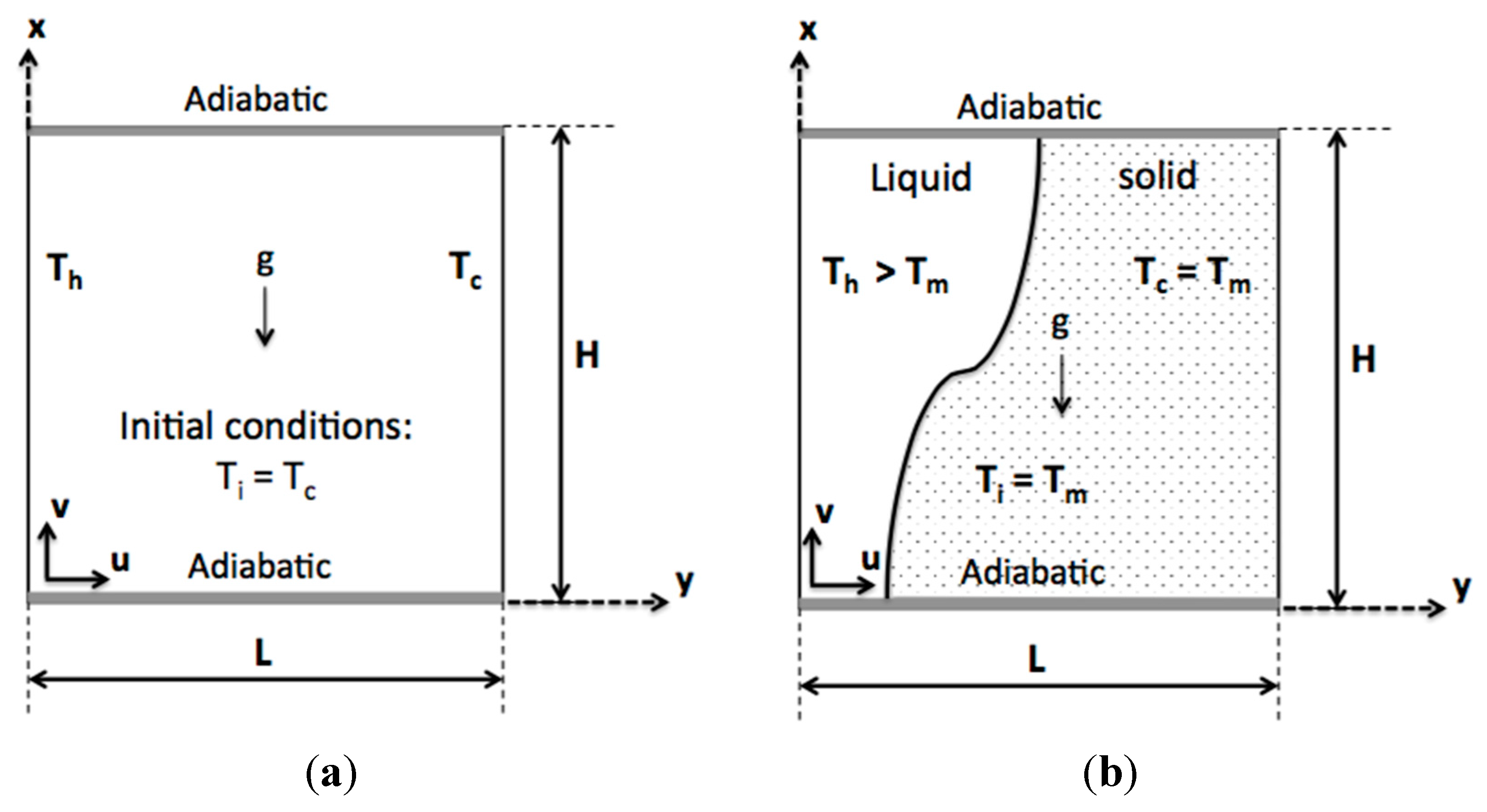
2.1. Mathematical Model

To solve the entropy generation problem due to natural convection under the conjectures stated above, the governing equations, in the transient state, are the following:

$$\nabla .\overrightarrow{U}=0$$

(1)

$$\frac{\text{D}\overrightarrow{U}}{\text{D}t}=-\nabla \left(\frac{p}{\mathsf{\rho }}\right)+\mathsf{\nu }{\nabla }^2\overrightarrow{U}-\mathsf{\beta }\left(T-T_0\right)\overrightarrow{g}$$

(2)

$$\frac{\text{D}T}{\text{D}t}=\mathsf{\alpha }{\nabla }^{2}T+S_h$$

(3)

where $\nabla$ is the nabla operator, $D/DT$ is the material derivative, $\overrightarrow{U}\left(U,V\right)$ is the velocity vector, $p$ is the pressure, $T$ is the temperature, $T_0$ is the reference temperature $(=(T_h+T_c)/2)$, $\mathsf{\rho }$ is the fluid density, $\mathsf{\nu }$ is the kinematic viscosity, $\mathsf{\beta }$ is the thermal expansion coefficient, $\mathsf{\alpha }$ is the thermal diffusivity, $\overrightarrow{g}$ is the gravity downward and $S_h(=\frac{L_f}{c_p}\frac{\partial \mathsf{\epsilon }}{\partial t})$ is the latent heat term (source or sink), $\mathsf{\epsilon }$ being the liquid fraction. Note that this quantity is negative for melting, positive for solidification and zero in the absence of a phase change.

To cast the above equations in a dimensional form, we employ the following dimensionless variables:

$$\tilde{t}=\frac{\mathsf{\alpha }t}{L^2},\left(X,Y\right)=\left(\frac{x}{L},\frac{y}{L}\right),\left(\tilde{U},\tilde{V}\right)=\left(\frac{uL}{\mathsf{\alpha }},\frac{vL}{\mathsf{\alpha }}\right),\tilde{p}={\left(\frac{L}{\mathsf{\alpha }}\right)}^2\frac{p}{\mathsf{\rho }},\tilde{T}=\frac{T-T_0}{T_h-T_c}$$

(4)

Equations (1)–(3), which govern the convective melting problem, then take the following dimensionless form:

$$\nabla .\overrightarrow{\tilde{U}}=0$$

(5)

$$\frac{\text{D}\overrightarrow{\tilde{U}}}{\text{D}\tilde{t}}=-\nabla \left(\tilde{p}\right)+\text{Pr}{\nabla }^2\overrightarrow{\tilde{U}}-\text{PrRa}\mathsf{\beta }\tilde{T}\overrightarrow{Y}$$

(6)

$$\frac{\text{D}\tilde{T}}{\text{D}\tilde{t}}={\nabla }^2\tilde{T}-St{e}^{-1}\partial \mathsf{\epsilon }/\partial \tilde{t}$$

(7)

where the symbol (˜) indicates that the quantity concerned is dimensionless and $\overrightarrow{\tilde{Y}}$ is the dimensionless vertical direction. Therefore, this problem involves the Prandtl number, the Rayleigh number and the Stefan number, defined by $\mathrm{Pr}=\mathsf{\nu }/\mathsf{\alpha }$, $Ra=g\mathsf{\beta }(T_h-T_c)L^3/\mathsf{\alpha }\mathsf{\nu }$, $Ste=c_p(T_h-T_c)/L_f$, respectively.

These equations are subjected to the following boundary (BCs) and initial conditions (ICs): The non-slip boundary condition for the hydrodynamic problem is applied at all cavity walls. For the thermal problem, the hot wall was kept with $\tilde{T}=0.5$ and the cold wall with $\tilde{T}=-0.5$. As for horizontal sides, the Neumann boundary condition (zero heat flux) is applied, i.e., $\partial \tilde{T}/\partial Y=0.0$. In the cavity, the initial conditions (ICs) are as follows: zero for the velocity field and $\tilde{T}=-0.5$ for the temperature field.

2.2. Entropy Generation

It should be noted that the entropy production in a system is a key thermodynamic parameter that can improve the performance of such a system. In other words, the determination of this parameter is used to analyze the total losses and, hence, to propose an optimization procedure. In the natural convection process, the entropy generation is associated with the heat transfer and with the fluid friction. According to Bejan [17], the local entropy generation ($S_{lo}$) can be expressed as:

$$S_{lo}=\frac{k}{{T_0}^2}{\left(\left|\nabla T\right|\right)}^2+\frac{2\mathsf{\mu }}{T_0}{S}_{ij}{S}_{ij}$$

(8)

where $k$ is the thermal conductivity of the fluid, $\mathsf{\mu }$ is the dynamic viscosity and $S_{ij}$ is the rate of the deformation tensor. In this expression, the first term (right-hand) is due to the heat transfer ($S_{l,h}$), while the second term is due to the viscous effects of the fluid ($S_{l,d}$). A dimensionless form of their expressions can be obtained as follows:

$${\tilde{S}}_{lo}={\tilde{S}}_{l,h}+{\tilde{S}}_{l,d}$$

(9)

with:

$${\tilde{S}}_{l,h}={\left(\left|\nabla \tilde{T}\right|\right)}^2,{\tilde{S}}_{l,d}=\mathsf{\phi }2{\tilde{S}}_{ij}{\tilde{S}}_{ij}\text{ and }\mathsf{\phi }=\frac{\mathsf{\mu }{T}_0}{k}{\left(\frac{\mathsf{\alpha }}{L\left(T_h-T_c\right)}\right)}^{\text{2}}$$

(10a)

Explicitly, ${\tilde{S}}_{l,h}$ and ${\tilde{S}}_{l,d}$can be expressed as:

$$\begin{array}{c}{\tilde{S}}_{l,h}={\left(\frac{\partial \tilde{T}}{\partial X}\right)}^2+{\left(\frac{\partial \tilde{T}}{\partial Y}\right)}^2\mathrm{ and}\\ {\tilde{S}}_{l,d}=\mathsf{\phi }\left[2\left({\left(\frac{\partial \tilde{U}}{\partial X}\right)}^2+{\left(\frac{\partial \tilde{V}}{\partial Y}\right)}^2\right)+{\left(\frac{\partial \tilde{U}}{\partial X}+\frac{\partial \tilde{V}}{\partial Y}\right)}^2\right],\mathrm{respectively}.\end{array}$$

(10b)

Here, $T_0$ is $(T_h+T_c)/2$; ${\tilde{S}}_{ij}$ is the dimensionless deformation rate; and $\mathsf{\phi }$ ($={\tilde{S}}_{l,d}/{\tilde{S}}_{l,h}$) is the irreversibility distribution ratio [6] that informs about the relative importance of the two mechanisms of irreversibility, i.e., ${\tilde{S}}_{l,d}$ and ${\tilde{S}}_{l,h}$. A further parameter that reflects the irreversibility distribution is the average Bejan number ($Be$) defined as [6,7]:

$$\text{Be}=\frac{{\tilde{S}}_{l,h}}{{\tilde{S}}_{lo}}$$

(11)

Therefore, $\text{Be}>>0.5$ indicates the dominance of the heat transfer irreversibility; $\text{Be}<<0.5$ reflects the dominance of the fluid viscous effects; and $\text{Be}=0.5$ means that the two phenomena do not compete.

The dimensionless total entropy generation (${\tilde{S}}_T$) is obtained via the integration of the local entropy generation (${\tilde{S}}_{lo}$) throughout the entire domain, namely:

$${\tilde{S}}_T={\displaystyle {\int }_V{\tilde{S}}_{lo}dv}$$

(12)

For the sake of clarity, henceforth, we will omit any symbol indicating dimensionless quantities.

3. Numerical Model

3.1. Thermal Lattice Boltzmann Equations

The TLBM consists of simulating the statistical behavior of a set of particles on a lattice with finite velocities. It stems from the discrete Boltzmann equation and allows providing macroscopic fluid properties, such as density, velocity, pressure, etc., through weighted averages, or moments, of the particle distribution for all discrete lattice velocities. The SRT-LBM (also called the Bhatnagar-Gross-Krook (BGK) model) for incompressible thermal flows builds on two distribution functions (DFs), $f_i$ and $g_i$, and their corresponding evolution equations [18,19]. As such, these are given here (Equations (13) and (14)) in the form of two steps, which are collision and streaming (advection) processes:

$$f_i\left(x+e_i,t+1\right)=f_i\left(x,t\right)-{\tau }_f^{-1}\left(f_i\left(x,t\right)-f_i^{eq}\left(x,t\right)\right)+\begin{array}{ccc}\text{Boussinesq\hspace{0.17em}force\hspace{0.17em}effect}& & \end{array}$$

(13)

$$g_i\left(x+e_i,t+1\right)=g_i\left(x,t\right)-{\tau }_h^{-1}\left(g_i\left(x,t\right)-g_i^{eq}\left(x,t\right)\right)+S_h^g$$

(14)

where $e_i$ is the microscopic particle velocity in the $i$-direction, ${\tau }_f$ and ${\tau }_h$ are the dimensionless relaxation times and $f_i^{eq}$ and $g_i^{eq}$are local equilibrium distributions functions that can be computed from:

$$f_i^{eq}=\mathsf{\rho }{\mathsf{\omega }}_i\left[1+\frac{3({\overrightarrow{e}}_i.\overrightarrow{u})}{c_s^2}+\frac{9{({\overrightarrow{e}}_i.\overrightarrow{u})}^2}{2c_s^4}-\frac{3(\overrightarrow{u}.\overrightarrow{u})}{2c_s^2}\right]$$

(15)

and:

$$g_i^{eq}=T{\mathsf{\omega }}_i\left[1+\frac{{\overrightarrow{e}}_i.\overrightarrow{u}}{c_s^2}\right]$$

(16)

where:

$${\mathsf{\omega }}_i=\{\begin{array}{l}4/9fori=0\\ 1/9fori=2,4,6,8\\ 1/36fori=0,3,5,9\end{array}\begin{array}{cc}& \end{array}\text{and}\begin{array}{cc}& \end{array}{e}_i=\{\begin{array}{l}\left(0,0\right)fori=0\\ \left(0,\pm 1\right)fori=2,4\\ \left(\pm 1,0\right)fori=1,3\\ \left(\pm 1,\pm 1\right)fori=5,6,7,8\end{array}$$

(17)

are, respectively, the weight coefficient and the velocity vector of the $\text{D2Q9}$ model; $\overrightarrow{u}\left(u,v\right)$ is the macroscopic velocity, with $u$ and $v$ representing velocities in the $x$- and $y$-directions, respectively. Note that the relaxation times ${\tau }_f$ and ${\tau }_h$ can be determined via ${\mathsf{\nu }}_{lattice}=c_s^2\mathsf{\Delta }t\left({\tau }_f-0.5\right)$ and ${\mathsf{\alpha }}_{lattice}=c_s^2\mathsf{\Delta }t\left({\tau }_h-0.5\right)$, $c_s$ being the lattice sound speed. It should be noted that, the lattice viscosity and diffusivity are selected so as to conform to the intended Prandtl number $\text{Pr\hspace{0.17em}}(={\mathsf{\nu }}_{lattice}/{\mathsf{\alpha }}_{lattice})$. Likewise, the additional force term related to Boussinesq force F_b is incorporated in the model by shifting the velocity field by a term of $F_b{\tau }_f/\mathsf{\rho }$, as proposed by Shan and Chen [20], where $F_b$ $\left(=-\mathsf{\beta }g\left(T-T_0\right)/\left(T_h-T_c\right)\right)$. By this treatment, there is no need to add a force term to the collision operator. On the other hand, in the g distribution function, the source term is treated as per the method proposed by Luo [21]. Hence, the resulting force in the LBM frame will be: $S_h^g=-{\mathsf{\omega }}_i{S}_h$ with $S_h$$\left(=St{e}^{-1}\partial \mathsf{\epsilon }/\partial t\right)$ being the source (or sink) term that handles the phase change.

The liquid fraction ($\mathsf{\epsilon }$) is computed from [15,16]:

$$\mathsf{\epsilon }=\{\begin{array}{l}0h<h_s=c_p{T}_m\\ \frac{h-h_s}{h_l-h_s}{h}_s\le h\le h_l=h_s+L_f\\ 1h>h_l\end{array}$$

(18)

where $h$ is the local enthalpy defined, at a time step j, by: $h^j=c_p{T}^j+\left({\mathsf{\epsilon }}^j-{\mathsf{\epsilon }}^{j-1}\right)L_f$.

It is useful to recall that in the current model, the solid and liquid phases are defined according to the liquid fraction value. Therefore, a mushy zone state is assigned when the value of ε is between zero and one. In this case, the velocity field is partially bounced back and the macroscopic velocity is modified as in Equation (19) [22]. The procedure of the implementation of the partial bounce-back approach is described in [23]. Note that, to implement BCs in the current method, we are led to convert them, at the mesoscopic level, in terms of the distribution function.

3.2. Boundary Conditions

In the LBM framework, implementing boundary conditions is a delicate task, because of the necessity of imposing conditions in terms of particle distributions $f_i$ and $g_i$.

For the velocity field, the non-slip boundary conditions are used for all four walls of the cavity. They are realized by the on-grid bounce-back (BB) boundary conditions. The procedure for this rule is to reverse the distribution function of the particle as $f_i(x_w\text{,}t+1)=f_j(x_w\text{,}t)$, where $x_w$ is a fluid node adjacent to the wall, and $i$ and $j$ represent two opposite lattice directions on the boundary site. Note that the BB conditions apply to the DF in non-parallel directions at a solid wall.

To specify a constant temperature at the left and right walls, we use the method proposed by Inamuro et al. [24]. Its principle is to substitute unknown DFs for a boundary point with local equilibrium values using an adjusted temperature to set the defined temperature at that point. Specifically, the adjusted temperature on the left side can be expressed as $T\prime =\frac{1}{1-3v_{w,x}}\left(T_h-{\displaystyle \sum g_k}\right)$, $v_{w,x}$ being the computed near-wall velocity, and $g_k$ represents a known distribution function. Hence, the unknown DFs $g_p$ are computed by $g_p=T\prime {\mathsf{\omega }}_i\left[1+{\overrightarrow{e}}_i.\overrightarrow{u}/c_s^2\right]$. As for the adiabatic BCs, the Neumann BCs are achieved using the BB boundary conditions for the distribution $g_i$, as prescribed for $f_i$.

3.3. Macroscopic Quantities

Finally, the basic thermo-hydrodynamic properties, such as density, $\mathsf{\rho }$, momentum density, $\mathsf{\rho }u$, and temperature, $T$, are defined as moments of the DFs, $f_i$ and $g_i$, as follows,

$$\mathsf{\rho }={\displaystyle \sum _{i=0}^{N=8}{f}_i},\mathsf{\rho }u={\displaystyle \sum _{i=0}^{N=8}{e}_i{f}_i},T={\displaystyle \sum _{i=0}^{N=8}{g}_i}$$

(19)

The velocity field is then modified in the mushy zone as,

$$u^{*}=\mathsf{\epsilon }u$$

(20)

This modified velocity is in accordance with the requirements of the partial bounce-back approach [23]. Accordingly, the flow in the mushy zone will be treated as flow in a porous medium and, thus, will be governed by the Darcy law, as proven by the derived analytical solutions in [23].

4. Model Validation

The current model has been implemented to carry out the 2D natural convection and the melting with natural convection. The obtained results have been compared with selected models that have adopted the same LBM scheme: Huber et al. [15] and Jourabian et al. [16].

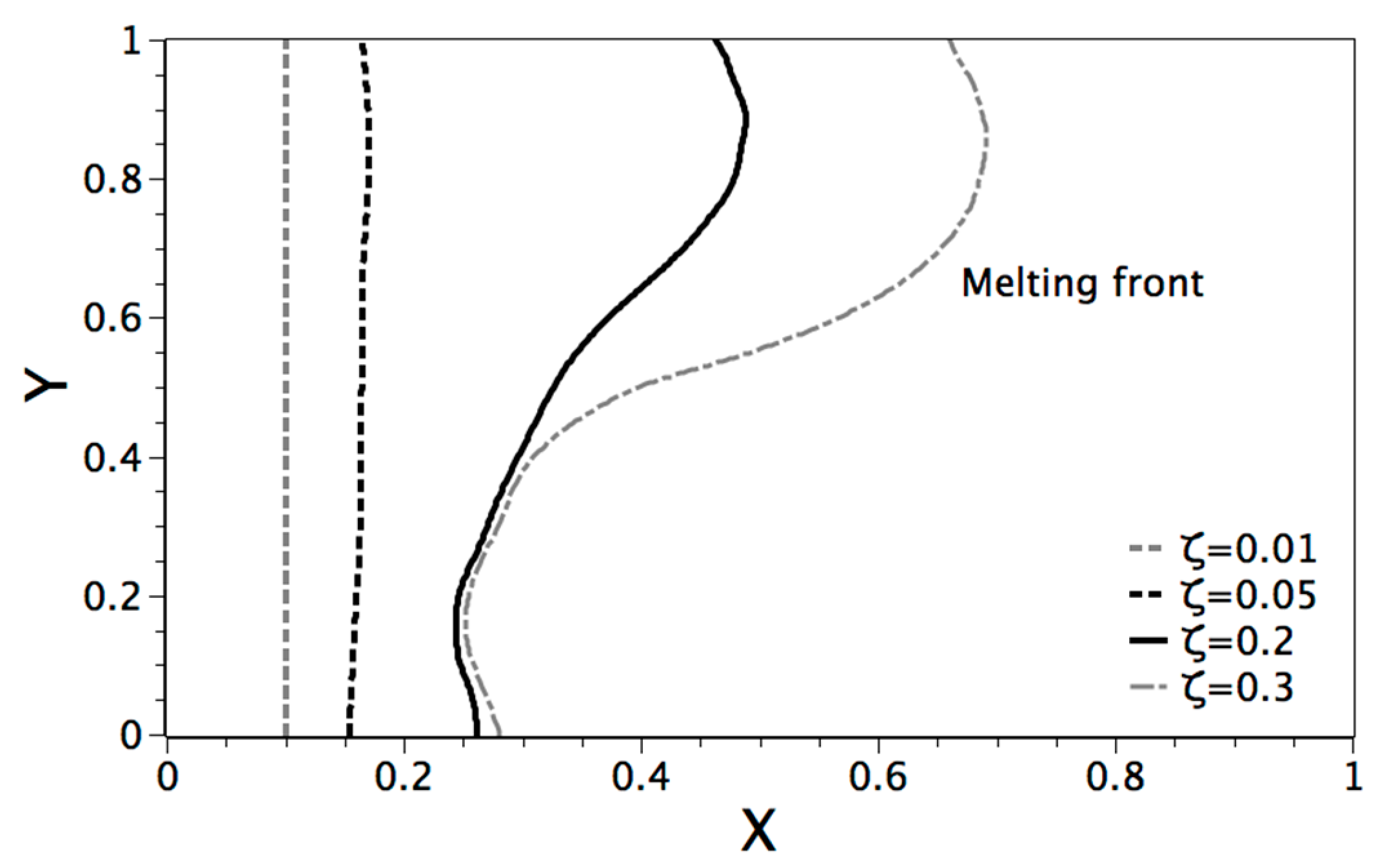
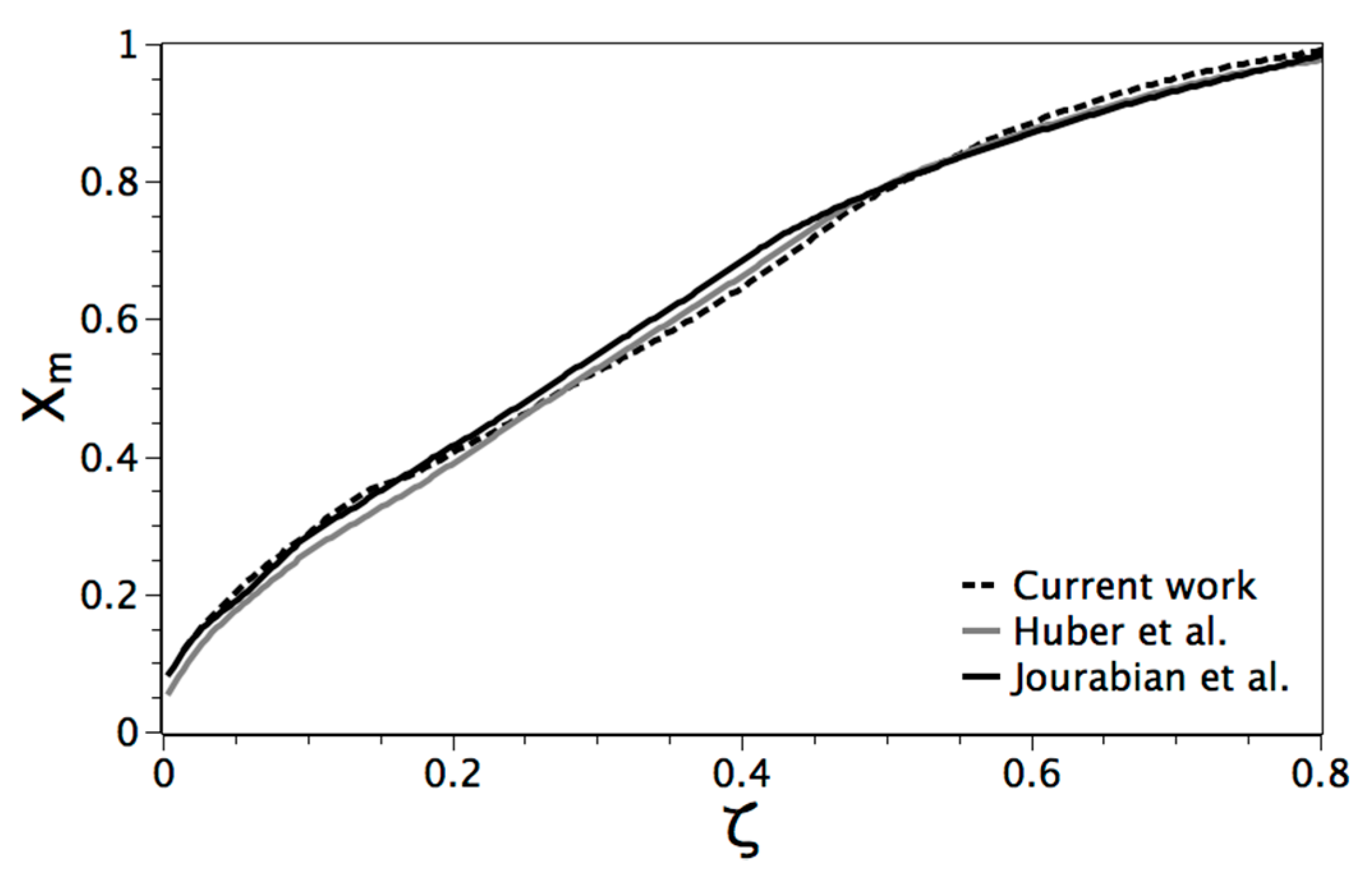
4.1. Melting with Convection

4.1.1. Comparison with Similar LBM Schemes

This subject was extensively treated in the literature with sound benchmarks presented in the works of Jany and Bejan [25] and Bertrand et al. [26], to name a few. However, for an LBM implementation, one can refer to the works of Miller et al. [27], Semma et al. [28] and, recently, Su and Davidson [29]. Note that our scheme is close to the bounce-back approach proposed by Huber et al. [15] and recently used by Jourabian et al. [16] to define the solid regime; however, our enhancement is to adopt a partial bounce-back approach rather than a full bounce-back. Hence, to check out our model, we resumed the convection melting problem handled in these references, keeping the same settings (see Table 1). Here, the key parameters governing this problem are the Stefan number, the Prandtl number, the Fourier number and the dimensionless time, whose definitions are: $\text{Ste}=c_P(T_h-T_c)/L_f$, $\text{Pr}=\mathsf{\nu }/\mathsf{\alpha }$, $\mathsf{\theta }=\tilde{t}=\mathsf{\alpha }t/L^2$ and ζ = Ste × θ, respectively.

Table 1. The melting benchmark parameters as in [15,16].

Parameter	Pr	Ra	Ste	Grid
Value	1	1.7 × 105	10	150 × 150

Table 1. The melting benchmark parameters as in [15,16].

Parameter	Pr	Ra	Ste	Grid
Value	1	1.7 × 105	10	150 × 150

Figure 2 shows the average position evolution of the melting front $X_m$ $\left(={\displaystyle {\int }_0^H{x}_{m}dY/H}\right)$ versus $\mathsf{\zeta }$, $x_m$ being the position of the melting front at each value of $Y$. From this figure, it is obvious that our current model reproduces quite closely the results already reported [15,16]. In addition, the shape of melting fronts confirms the expected scaling theory proposed by Jany and Bejan [25].

As time proceeds, the upper portion recedes faster due to convection, while the lower part remains upright while being dominated by the conduction ($\mathsf{\zeta }=0.05$ of Figure 3). However, thereafter, the advection part expands to govern the entire height of the front ($\mathsf{\zeta }=0.2$ and $0.3$ of Figure 3). At the end, a shrinking solid regime is attained as the front reaches the cold wall.

Figure 2. The average position evolution of the melting front versus $\mathsf{\zeta }$. Comparison with the results of [15,16].

Figure 2. The average position evolution of the melting front versus $\mathsf{\zeta }$. Comparison with the results of [15,16].

Figure 3. Position and shape of the melting front at different dimensionless times $\mathsf{\zeta }$.

Figure 3. Position and shape of the melting front at different dimensionless times $\mathsf{\zeta }$.

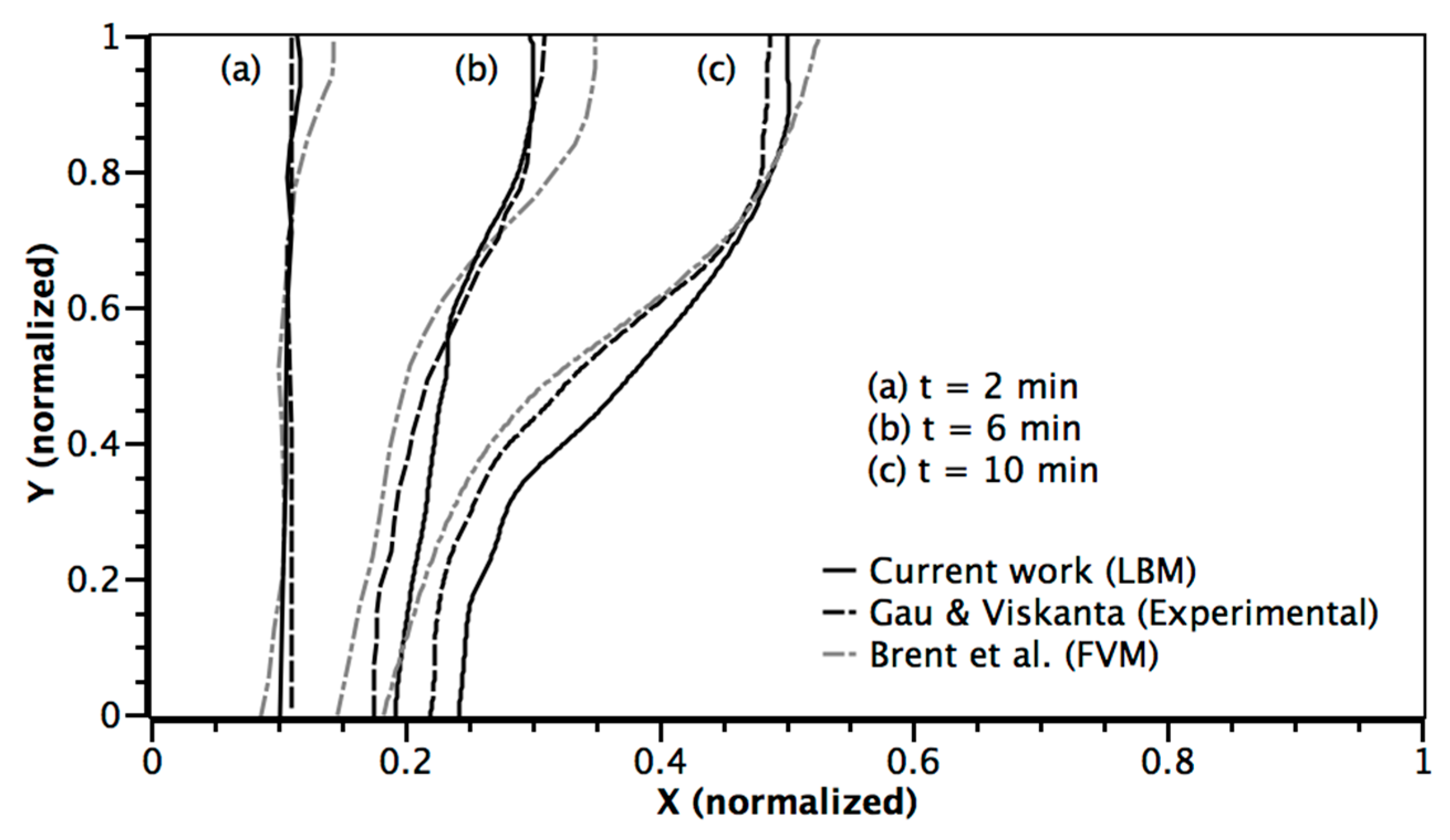
4.1.2. Comparison with Experimental Results and the Finite Volume Method

To further check the model considered here, we conducted a comparison with the experimental results of Gau and Viskanta available for Gallium [30]. Moreover, we compared our results for the same problem (melting of a pure Gallium) with the finite volume method (FVM), based on the enthalpy-porosity approach, proposed by Brent et al. [31]. The considered problem seeks to examine the 2D melting of pure Gallium in a rectangular cavity heated from one side, while its other sides are adiabatic. The used parameters are gathered in Table 2.

Table 2. The melting benchmark parameters of pure Gallium [30,31].

Parameter	Pr	Ra	Ste	Aspect Ratio
Value	0.021	6 × 105	0.039	H/L = 1.4

Table 2. The melting benchmark parameters of pure Gallium [30,31].

Parameter	Pr	Ra	Ste	Aspect Ratio
Value	0.021	6 × 105	0.039	H/L = 1.4

In their work, Gau and Viskanta [30] presented detailed traces of the morphology of the melt front at various times. For the propagation of the melting front using this model, our obtained findings via the current model are compared to the results already published (see [30,31]). This comparison is exhibited in Figure 4. As inferred, our results are close to the experimental data, especially in the upper portion of the cavity. However, more discrepancy is exhibited in the lower portion. Thereby, this comparison demonstrates the effectiveness of the approach used here for the melting by convection problems.

Figure 4. Position and shape of the melting front at selected times: (a) $t=2$ min, (b) 6 min and (c) 10 min compared to [30,31].

Figure 4. Position and shape of the melting front at selected times: (a) $t=2$ min, (b) 6 min and (c) 10 min compared to [30,31].

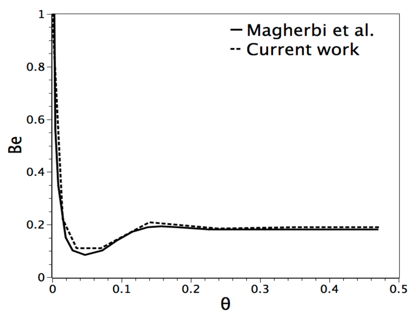
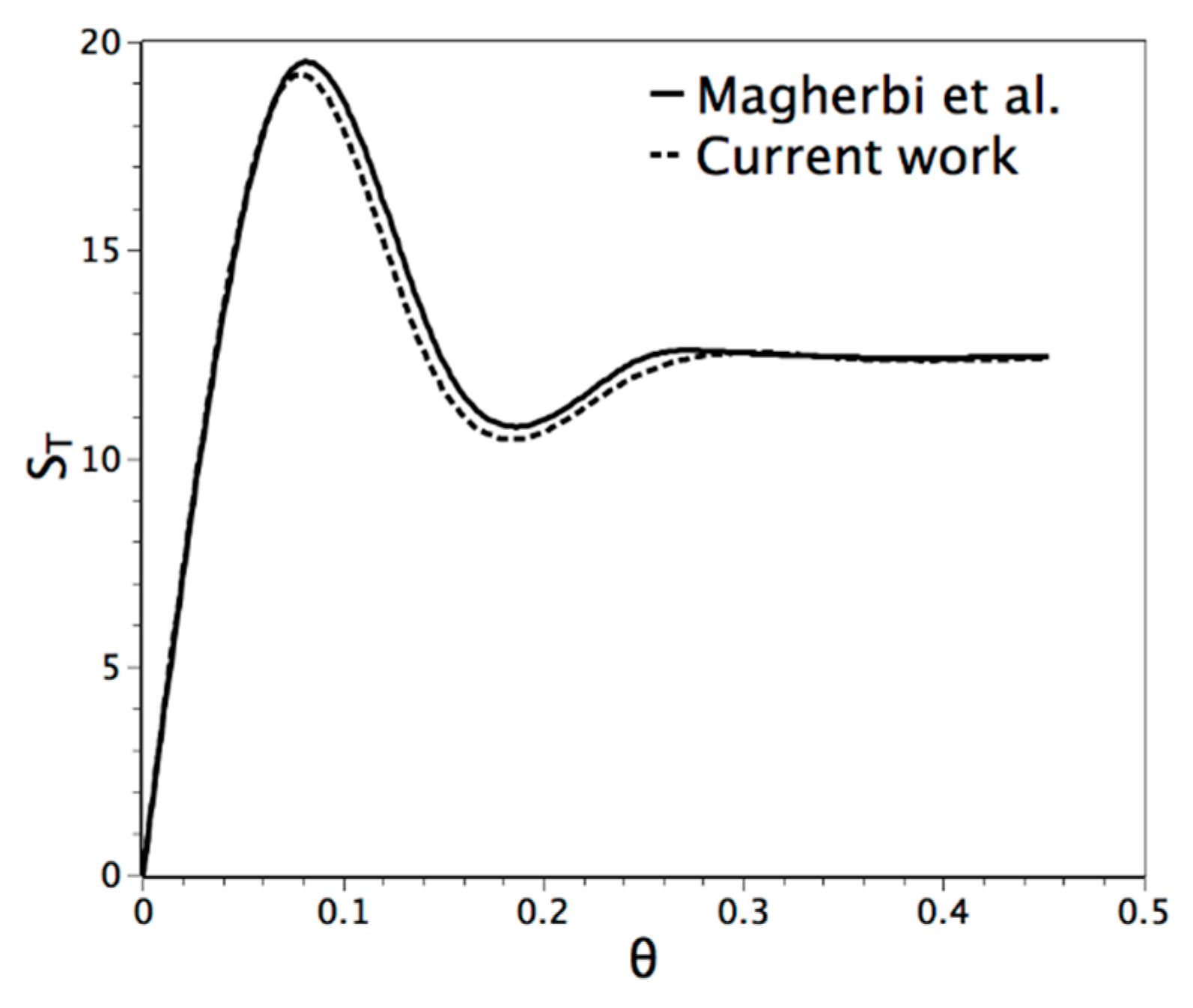
4.2. Entropy Generation

Unless otherwise stated, the entropy generation is computed by integrating the local entropy production over the whole simulation domain. To achieve this, we have considered the case already handled by Magherbi et al. [6]. Here, too, we have adopted the same parameters as those of these authors (see Table 3). Figure 5 and Figure 6 depict temporal evolutions of the total entropy generation and the Bejan number, respectively. It should be noted that this latter parameter remains a constant for each simulation. As can be seen, our results match those of [6]. Note that these two parameters exhibit oscillations before reaching the steady state. To sum up, we can state that such a comparison verifies and validates the present model.

Table 3. The entropy generation parameters as in [6].

Parameter	Pr	Ra	φ	ΔT
Value	0.7	104	10−3	1.0

Table 3. The entropy generation parameters as in [6].

Parameter	Pr	Ra	φ	ΔT
Value	0.7	104	10−3	1.0

Figure 5. Total entropy production vs. dimensionless time $\mathsf{\theta }$ ($=\mathsf{\alpha }t/L^2$).

Figure 5. Total entropy production vs. dimensionless time $\mathsf{\theta }$ ($=\mathsf{\alpha }t/L^2$).

Figure 6. Bejan number (Be) vs. dimensionless time $\mathsf{\theta }$.

Figure 6. Bejan number (Be) vs. dimensionless time $\mathsf{\theta }$.

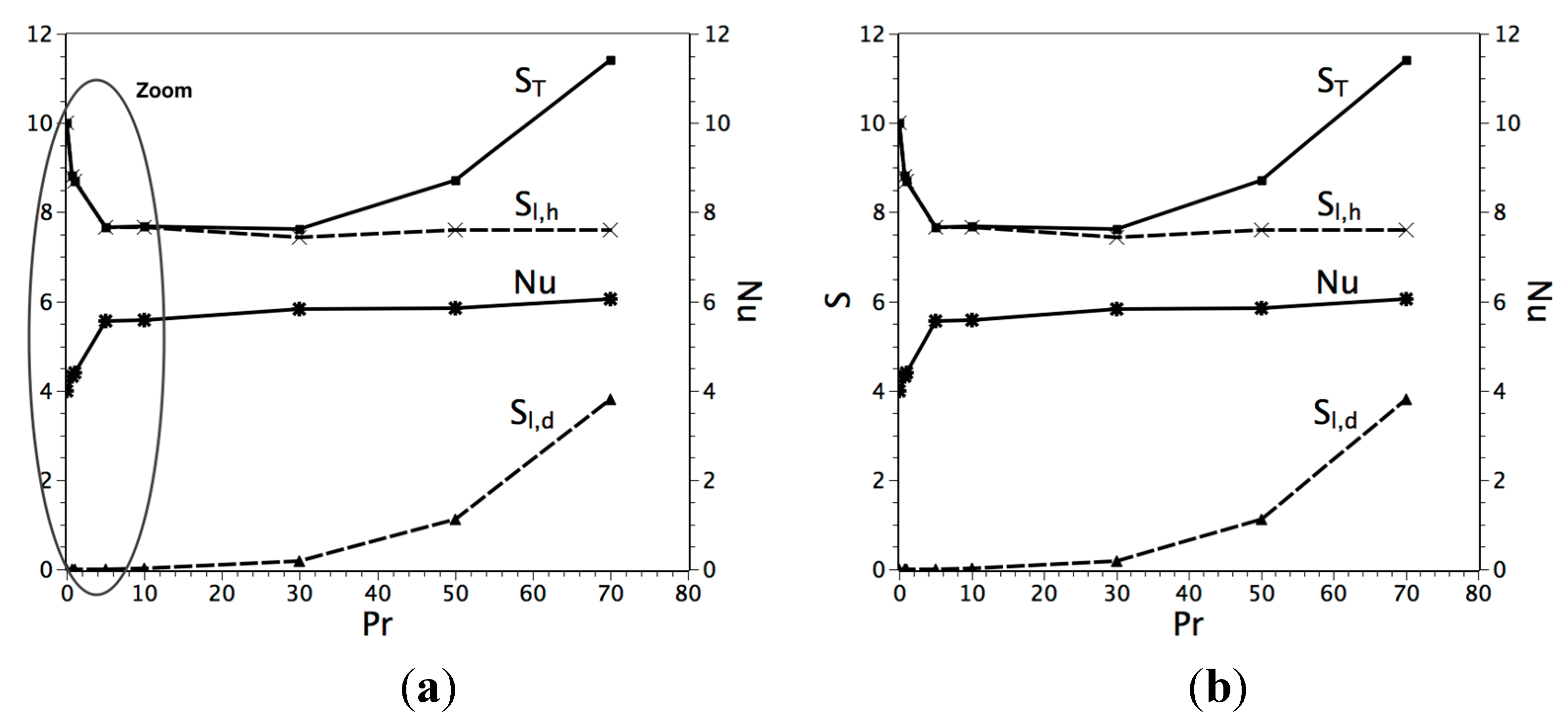
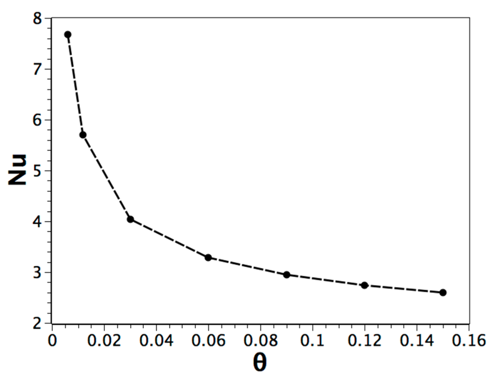
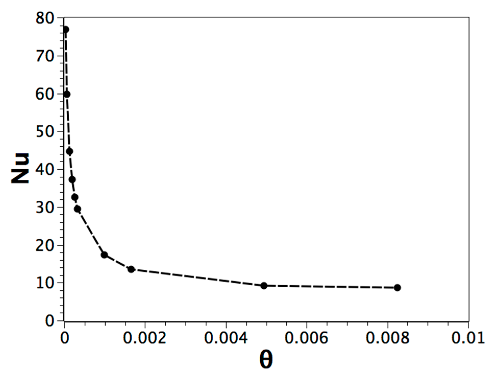
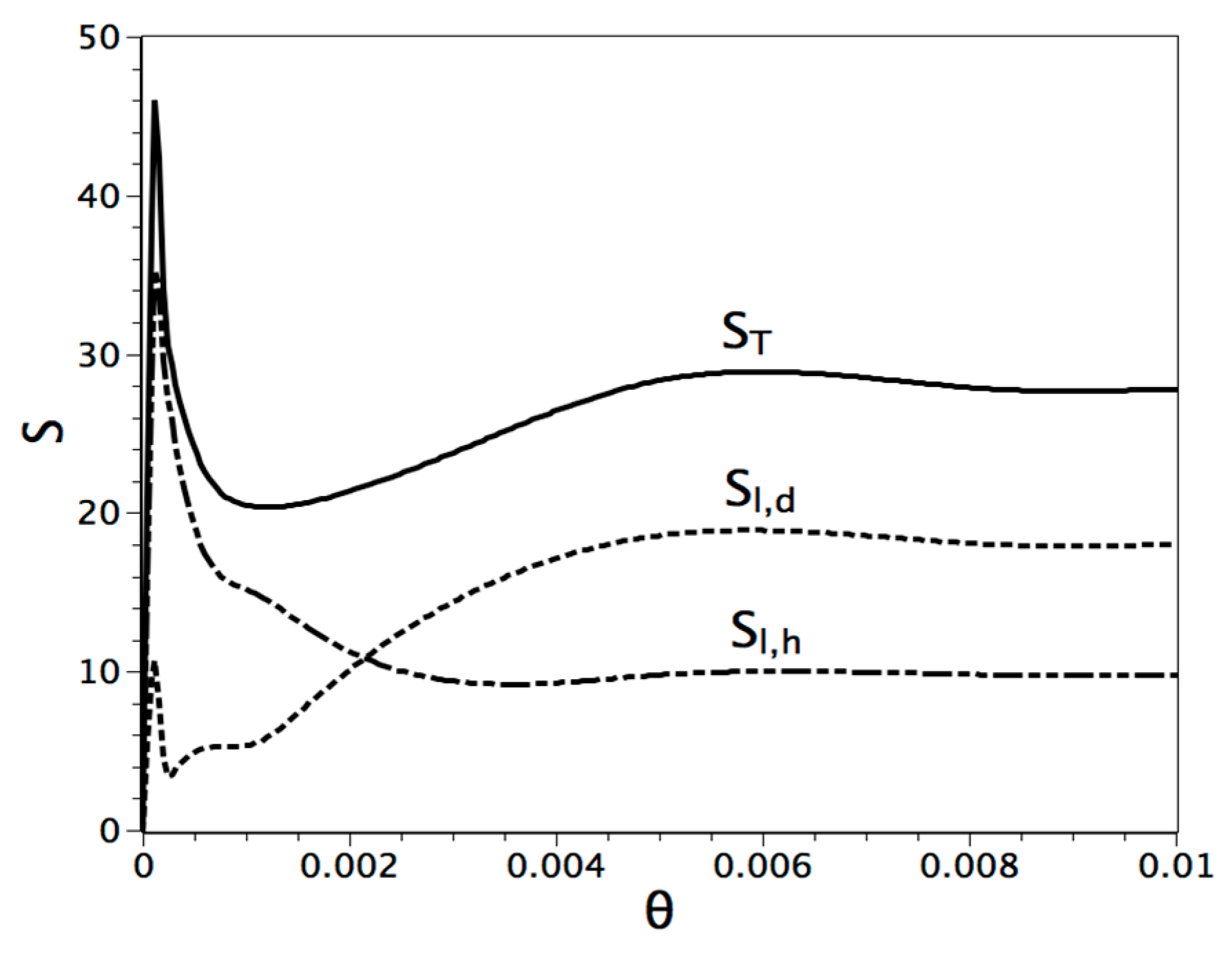
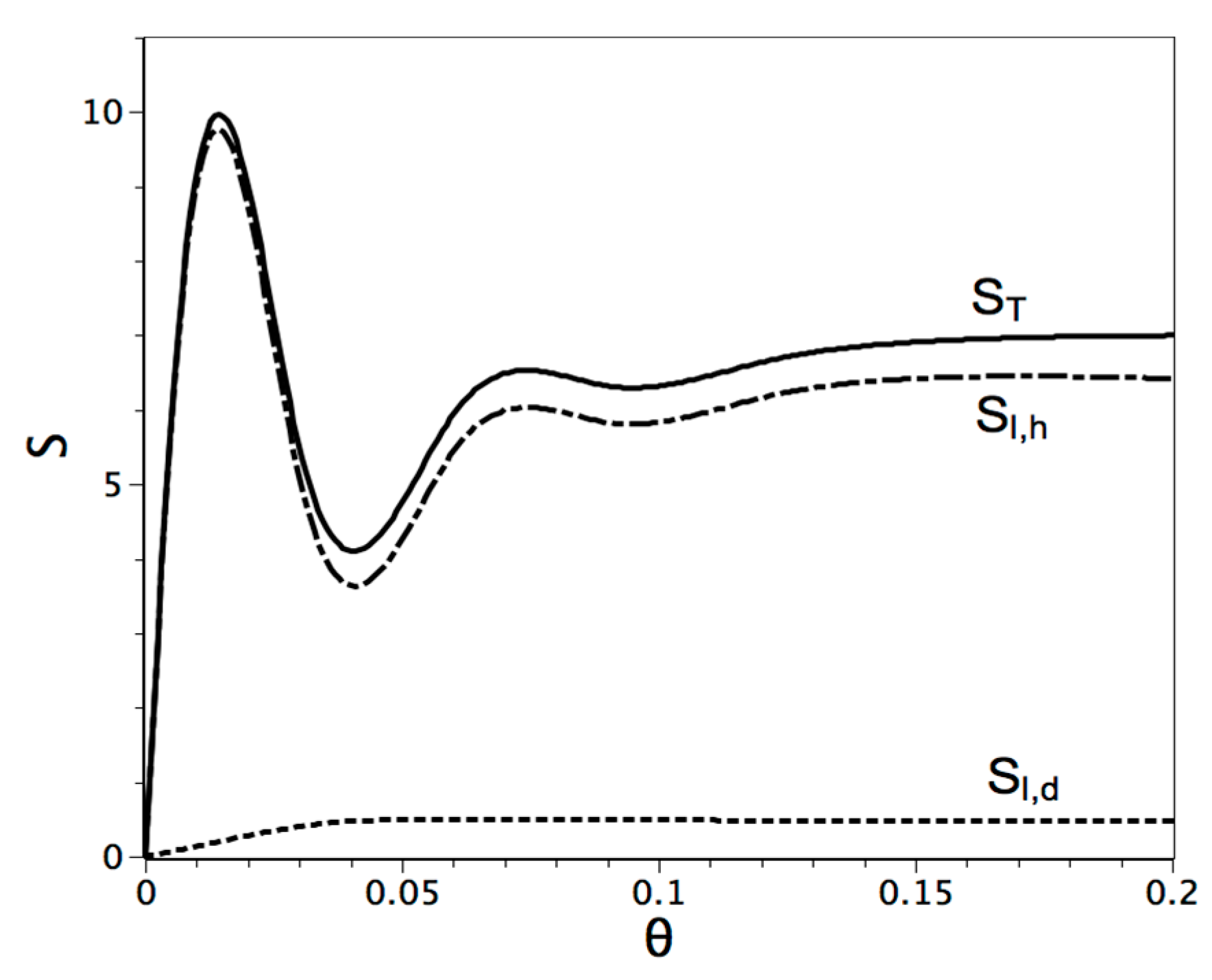
5. Results and Analysis

It is useful to recall that the numerical prediction of heat transfer and entropy generation in a 2D square cavity is the main concern of this work. This has been performed for different $\text{Pr}$ from $\text{Pr}={2.10}^{-2}$ to $\text{Pr}=70$ and at a fixed Rayleigh number ($\text{Ra}={10}^4$) with irreversibility distribution $\mathsf{\phi }={10}^{-7}$. Figure 7a, b illustrates the evolution of $S_T$, $S_{l,d}$, $S_{l,h}$ and $Nu$ (on the hot wall) according to the Prandtl number. A careful review of this figure shows that the effect of $\mathrm{Pr}$ on $S_{l,h}$ and $Nu$ is obvious for low values of $\text{Pr}$. For small $\text{Pr}$ ($<1$), the thermal boundary layer becomes very thin, indicating that the heat transfer irreversibility ($S_{l,h}$) is dominative in the vicinity of boundaries, although the inner part of the simulation domain is dominated by the fluid friction irreversibility. We find that $S_{l,h}$ decreases quite sharply until $\text{Pr}=5$, from which it reaches its constant value, which stays up to 70. As for $S_{l,d}$, it remains insignificant until $\text{Pr}=30$, from which it starts to increase substantially. Furthermore, the effect of $\text{Pr}$ on $S_{l,h}$ is more significant for the range of $0.02<\text{Pr}<30$. Beyond $\text{Pr}=30$, the effect of $\text{Pr}$ on $S_{l,d}$ becomes very important. This is well reflected in Figure 8, where we plot the influence of the Bejan number versus $\text{Pr}$. On the other hand, the $\text{Nu}$ varies inversely to $S_{l,h}$, especially in the case of low $\mathrm{Pr}$. This shows that an enhanced heat transfer coefficient contributes to decreasing losses in the system.

Figure 7. (a) $S_T$, $S_{l,h}$, $S_{l,d}$ and $\text{Nu}$ vs. $\text{Pr}$; (b) zoom on $S_T$, $S_{l,h}$, $S_{l,d}$ and $\text{Nu}$ vs. $\text{Pr}$ (= 0.02 till 10).

Figure 7. (a) $S_T$, $S_{l,h}$, $S_{l,d}$ and $\text{Nu}$ vs. $\text{Pr}$; (b) zoom on $S_T$, $S_{l,h}$, $S_{l,d}$ and $\text{Nu}$ vs. $\text{Pr}$ (= 0.02 till 10).

Figure 8. Bejan number vs. Prandtl number.

Figure 8. Bejan number vs. Prandtl number.

In what follows, we focus on the transient entropy generation with phase change. It is well known that during melting, the material undergoes an isothermal phase with a release of latent heat. Here, we ask the question about the effect of this phenomenon on the evolution of the generation of entropy through time. For this purpose, two models with different $\mathrm{Pr}$ have been investigated. Following this simulation, a comparison of the losses between the transfer of sensible and latent heat is carried out.

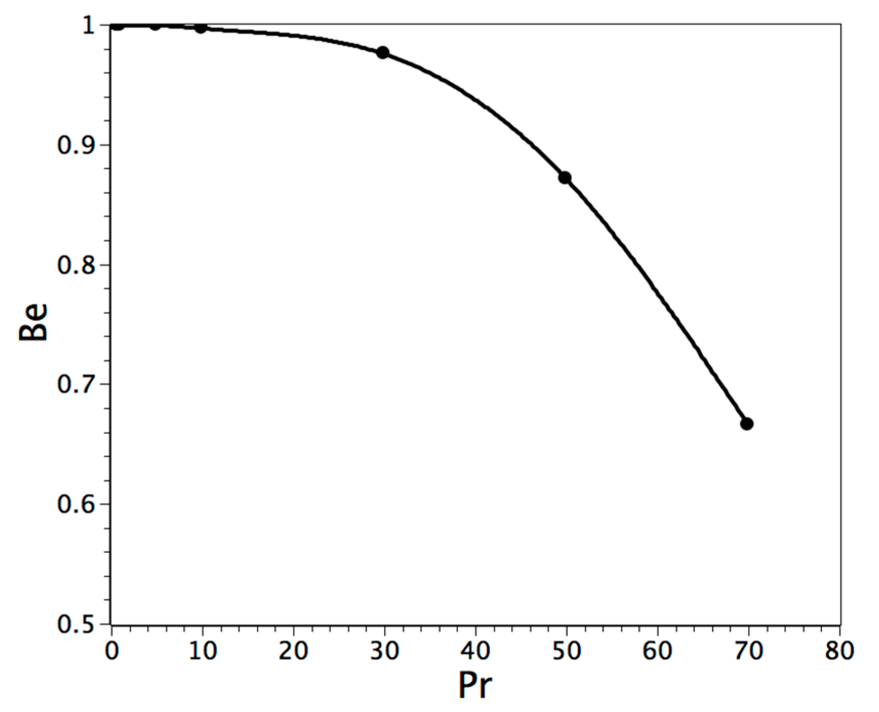
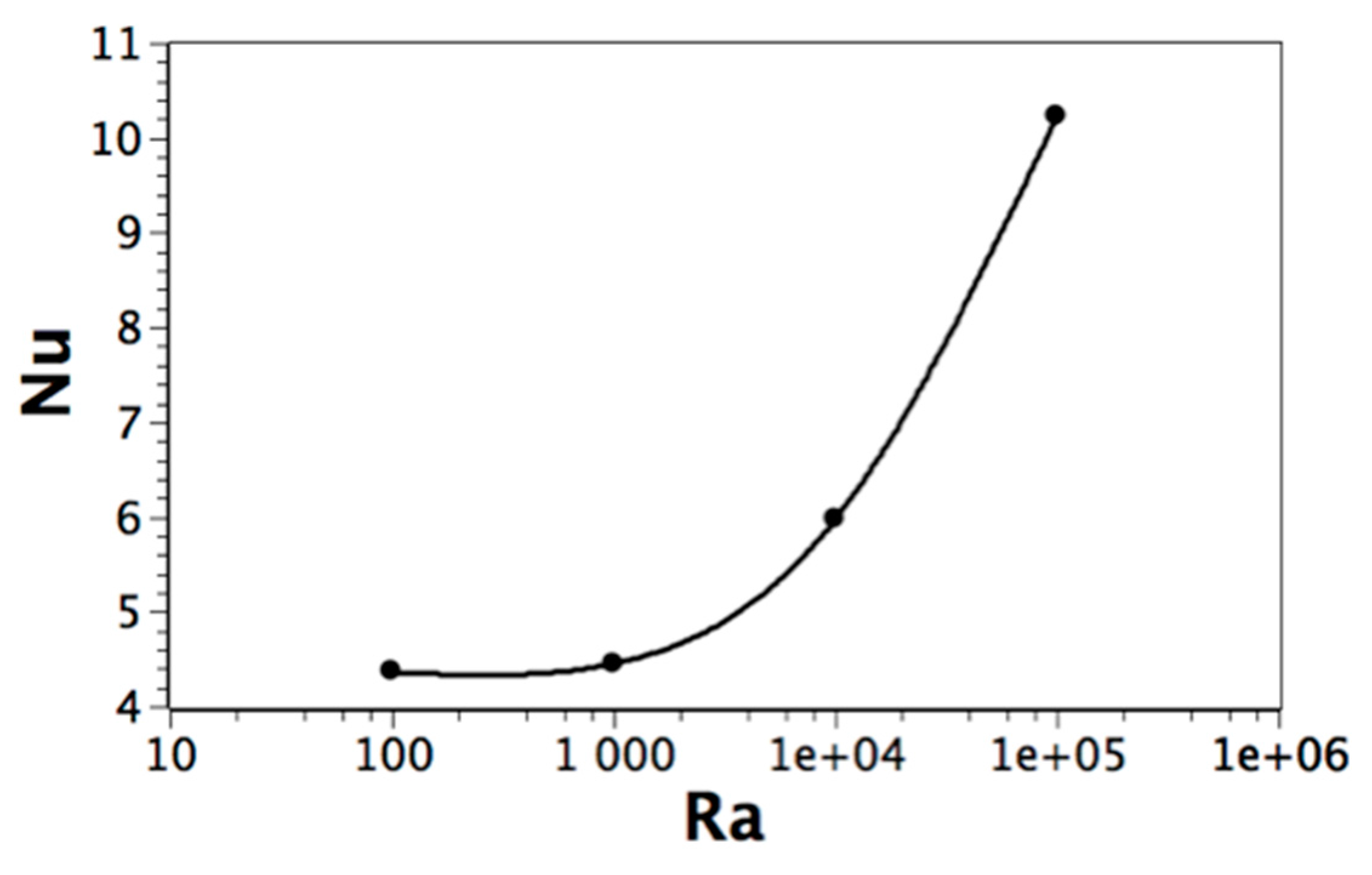
Single-Phase and Solid-Liquid Phase Change with High Prandtl Number

To investigate the effect of phase change on the entropy generation, we conduct the simulations on octadecane, whose parameters are summarized in Table 4. Octadecane is known for having a relatively high convective coefficient. This increases the heat transfer and the fluid velocities. The generation of latent heat during the melting process increases the energy stored in the system. However, we will investigate whether this is provoked by an increase or decrease in the total entropy generation.

Table 4. The simulation parameters of Octadecane.

Parameter	Pr	Ra	φ	Ste (Figure 1b)
Value	50	104 − 105	10−5	1.0

Table 4. The simulation parameters of Octadecane.

Parameter	Pr	Ra	φ	Ste (Figure 1b)
Value	50	104 − 105	10−5	1.0

Figure 9 and Figure 10 show the temporal evolution of the entropy generation during heat transfer with no phase change (the problem described in Figure 1a). Here, these quantities further exhibit oscillations due to the high value of $\text{Ra}$ before reaching their asymptotic values. Such behavior is due to boundary conditions [3]. At first, the isotherms are almost vertical and parallel to the walls since the heat transfer is dictated by the conduction. As time passes, the advection mode becomes more dominant and distorts isotherms, inducing vertical temperature gradients. This will result in a decrease in horizontal temperature gradients, which eventually become locally negative. Consequently, the central streamline elongates to give rise to a second eddy. Thus, for smaller Rayleigh numbers, the steady state is sufficiently close to the equilibrium state, allowing the system to return towards the steady state. Thereby, Prigogine’s theorem of minimum entropy production is satisfied. However, for larger $\text{Ra}$’s, the equilibrium state being relatively far, the system oscillates increasingly. Note that this finding has already been reported by Magherbi [6].

Figure 9. Entropy generations with no phase change (problem in Figure 1a) for $\text{Pr}=50$ and $\text{Ra}={10}^5$.

Figure 9. Entropy generations with no phase change (problem in Figure 1a) for $\text{Pr}=50$ and $\text{Ra}={10}^5$.

Figure 10. Entropy generations with no phase change (problem in Figure 1a) for $\text{Pr}=50$ and $\text{Ra}={10}^5$.

Figure 10. Entropy generations with no phase change (problem in Figure 1a) for $\text{Pr}=50$ and $\text{Ra}={10}^5$.

We also observe that the steady state is reached sooner at larger $\text{Ra}$ (Figure 10), whereas at lower $\text{Ra}$ (Figure 9), oscillations of transient entropy generation are both apparent and smooth. This is due to the effect of the heat transfer coefficient. For more information on this, we plot in Figure 11 and Figure 12 the Nusselt number (Nu) versus the dimensionless time for the cases of $\text{Ra}={10}^4$ and ${10}^5$. The rate of variation of Nu affects the losses due to heat transfer. However, the increase of Nu values at steady state has a significant effect on the fluid velocities and, hence, fluid friction losses. Figure 13 shows the Nusselt number (Nu) versus the different values of (Ra). We deduce that somewhere after $\text{Ra}={10}^4$, the heat transfer coefficient at steady state increases dramatically. This leads to higher fluid velocities and, therefore, higher fluid friction losses, as revealed in Figure 10.

Figure 14 shows the temporal variation of the entropy generation in the case of melting with convection. Note that the entropy generation oscillates at the beginning with about a 25% decrease compared to the case of heat transfer with no phase change. Nevertheless, at the steady state, the total entropy generation decreases by more than 50% with the presence of phase change and latent heat dissipation, as illustrated in Figure 14. This is also justified by tracing the Nu versus time in Figure 15. The values of Nu decrease in comparison with the case of no phase change. The reason for that is that the fluid volume increases with time as the melting front recedes. Here, we note that, in reality, we can define a Rayleigh number at each time step depending on the position of the melting front ($X_m$) by ${\text{Ra}}_m=\mathsf{\beta }g\mathsf{\Delta }T{\left(X_m\right)}^3/\mathsf{\alpha }\mathsf{\nu }$.

Figure 11. Nu versus dimensionless time (see Figure 1a) for $\text{Pr}=50$ and $\text{Ra}={10}^5$.

Figure 11. Nu versus dimensionless time (see Figure 1a) for $\text{Pr}=50$ and $\text{Ra}={10}^5$.

Figure 12. Nu versus dimensionless time (see Figure 1a) for$\text{Pr}=50$ and $\text{Ra}={10}^5$.

Figure 12. Nu versus dimensionless time (see Figure 1a) for$\text{Pr}=50$ and $\text{Ra}={10}^5$.

Figure 13. Variation of Nu with Ra (problem in Figure 1a) for $\text{Pr}=50$.

Figure 13. Variation of Nu with Ra (problem in Figure 1a) for $\text{Pr}=50$.

Figure 14. Entropy generation for melting with convection (problem in Figure 1b) for $\text{Pr}=50$ and $\text{Ra}={10}^5$.

Figure 14. Entropy generation for melting with convection (problem in Figure 1b) for $\text{Pr}=50$ and $\text{Ra}={10}^5$.

Figure 15. Nu versus dimensionless time (problem in Figure 1b) for $\text{Pr}=50$ and $\text{Ra}={10}^5$.

Figure 15. Nu versus dimensionless time (problem in Figure 1b) for $\text{Pr}=50$ and $\text{Ra}={10}^5$.

It also can be stated that, as the melting interface proceeds, the total entropy generation keeps decreasing until reaching a stable state. This is likely due to the relatively low diffusivity, where the system exhibits higher losses due to the small distance between temperature gradients at the beginning of the melting, as illustrated in Figure 16.

Figure 16. Entropy generation versus $X_m$ during latent heat transfer with $\text{Pr}=50$ and Ra = 10⁵.

Figure 16. Entropy generation versus $X_m$ during latent heat transfer with $\text{Pr}=50$ and Ra = 10⁵.

6. Conclusions

This study deals with the analysis of entropy generation during natural convection within a differentially-heated cavity. In this process, the entropy generation for sensible and latent heat transfers has been investigated at different Prandtl numbers via a thermal lattice Boltzmann method. The influences of the Rayleigh number, the Prandtl number and the irreversibility distribution on the entropy generation are assessed. Within the range considered for the key problem parameters, it is shown that entropy generation is controlled by the heat transfer losses for low $\text{Pr}$. However, for large for large Prandtl numbers, the variation of $S_T$ is dominated by $S_{l,d}$, because $S_{l,h}$ has reached its asymptotic value. In addition, it turned out that the increase of the Rayleigh number is required to ensure better heat transfer. Yet, the system will be prone to more losses. Likewise, a suitable choice of the Rayleigh number ($\text{Ra}$) and the irreversibility distribution ($\mathsf{\phi }$) will permit getting an indication of a possible optimum design of the enclosure. Moreover, the presence of the latent heat state decreases the overall thermodynamic losses while increasing the quantity of heat transferred.

References

1. Sheikholeslami, M.; Ellahi, R. Electrohydrodynamic nanofluid hydrothermal treatment in an enclosure with sinusoidal upper wall. Appl. Sci. 2015, 5, 294–306. [Google Scholar] [CrossRef]
2. Zeeshan, A.; Ellahi, R.; Hassan, M. Magnetohydrodynamic flow of water/ethylene glycol based nanofluids with natural convection through porous medium. Eur. Phys. J. Plus 2014. [Google Scholar] [CrossRef]
3. Sheikholeslami, M.; Ellahi, R.; Mohsan, H.; Soleimani, S. A study of natural convection heat transfer in a nanofluid filled enclosure with elliptic inner cylinder. Int. J. Numer. Methods Heat Fluid Flow 2014, 24, 1906–1927. [Google Scholar] [CrossRef]
4. Qi, C.; He, Y.; Yan, S.; Tian, F.; Hu, Y. Numerical simulation of natural convection in a square enclosure filled wih nanofluid using the two-phase lattice Boltzmann method. Nanoscale Res. Lett. 2013, 8, 1–56. [Google Scholar] [CrossRef] [PubMed]
5. Singh, V.; Aute, V.; Radermacher, R. Usefulness of entropy generation minimization through a heat exchanger modeling tool. In Proceedings of the International Refrigeration and Air Conditioning Conference, Poznan, Poland, 15–17 October 2008; p. 958.
6. Bejan, A. Entropy Generation Minimization; CRC Press: Boca Raton, FL, USA; New York, NY, USA, 1996. [Google Scholar]
7. Maghrebi, M.; Abbassi, H.; Brahim, A.B. Entropy generation at the onset of natural convection. Int. J. Heat Mass Transf. 2003, 46, 3441–3450. [Google Scholar] [CrossRef]
8. Abu-Hijleh, B.A.K.; Abu-Qudais, M.; Abu-Nada, E. Numerical prediction of entropy generation due to natural convection from a horizontal cylinder. Energy 1999, 24, 327–333. [Google Scholar] [CrossRef]
9. Mahmud, S.; Island, A.K.S. Laminar free convection and entropy generation inside an inclined wavy enclosure. Int. J. Therm. Sci. 2003, 42, 1003–1012. [Google Scholar] [CrossRef]
10. Ellahi, R.; Hassan, M.; Zeeshan, A. Shape effects of nanosize particles in Cu­H2O nanofluid on entropy generation. Int. J. Heat Mass Trans. 2015, 81, 449–456. [Google Scholar] [CrossRef]
11. Chen, S.; Doolen, G.D. Lattice Boltzmann method for fluid flows. Annu. Rev. Fluid Mech. 1998, 30, 329–364. [Google Scholar] [CrossRef]
12. Shi, Y.; Zhao, T.S.; Guo, Z.L. Thermal lattice Bhatnagar-Gross-Krook model for flows with viscous heat dissipation in the incompressible limit. Phys. Rev. E 2004, 70, 0663101–06631010. [Google Scholar]
13. Li, Q.; He, Y.L.; Wang, Y.; Tang, G.H. An improved thermal lattice Boltzmann model for flows without viscous heat dissipation and compression work. Int. J. Mod. Phys. C 2008, 19, 125–150. [Google Scholar] [CrossRef]
14. Sheikholelasmi, M.; Bandpy, M.G.; Ellahi, R.; Zeeshan, A. Simulation of MHD CuO­water nanofluid flow and convective heat transfer considering Lorentz forces. J. Magn. Magn. Mater. 2014, 369, 69–80. [Google Scholar] [CrossRef]
15. Huber, C.; Parmigiani, A.; Chopard, B.; Manga, M.; Bachmann, O. Lattice Boltzmann model for melting with natural convection. Int. J. Heat Fluid Flow 2008, 29, 1469–1480. [Google Scholar] [CrossRef]
16. Jourabian, M.; Farhadi, M.; Darzi, A.A.R. Convection-dominated melting of phase change material in partially heated cavity: Lattice Boltzmann study. Heat Mass Transf. 2013, 49, 555–565. [Google Scholar] [CrossRef]
17. Bejan, A. Fundamentals of exergy analysis, entropy-generation minimization, and the generation of flow architecture. Int. J. Energy Res. 2002, 26, 545–565. [Google Scholar] [CrossRef]
18. Mohamad, A.A.; Bennacer, R.; El-Ganaoui, M. Double dispersion, natural convection in an open end cavity simulation via lattice Boltzmann method. Int. J. Therm. Sci. 2010, 49, 1944–1953. [Google Scholar] [CrossRef]
19. Sidik, N.A.C.; Razali, S.A. Lattice Boltzmann method for convective heat transfer of nanofluids–A review. Renew. Sustain. Energy Rev. 2014, 38, 864–875. [Google Scholar] [CrossRef]
20. Chen, H.; Shan, X. Simulation of nonideal gases and gas-liquid phase transitions by the lattice Boltzmann equation. Phys. Rev. E 1994, 49, 2941–2948. [Google Scholar]
21. Luo, L.-S. Lattice-Gas Automata and Lattice Boltzmann Equations for Two-Dimensional Hydrodynamics. Ph.D. Thesis, Georgia Institute of Technology, Atlanta, GA, USA, 1993. [Google Scholar]
22. Sukop, M.C.; Thorne, D.T. Lattice Boltzmann Modeling: An introduction for Geoscientists and Engineers; Springer: Berlin, Germany, 2006. [Google Scholar]
23. Yehya, A.; Naji, H.; Sukop, M.C. Simulating flows in multi-layered and spatially-variable permeability media via a new Gray Lattice Boltzmann model. Comp. Geotech. 2015, 70, 150–158. [Google Scholar] [CrossRef]
24. Inamuro, T.; Yoshino, M.; Inoue, H.; Mizuno, R.; Ogino, F. A lattice Boltzmann method for a binary miscible fluid mixture and its application to a heat-transfer problem. J. Comput. Phys. 2002, 179, 201–215. [Google Scholar] [CrossRef]
25. Jany, P.; Bejan, A. Scaling theory of melting with natural convection in an enclosure. Int. J. Heat Mass Transf. 1988, 31, 1221–1235. [Google Scholar] [CrossRef]
26. Bertrand, O.; Binet, B.; Combeau, H.; Couturier, S.; Delanno, Y.; Gobin, D.; Lacroix, M.; Quéré, P.L.; Médale, M.; Mencinger, J.; et al. Melting driven by natural convection. A comparison exercise: First results. Int. J. Therm. Sci. 1999, 38, 5–26. [Google Scholar] [CrossRef]
27. Miller, W.; Succi, S. A lattice Boltzmann model for anisotropic crystal growth from melt. J. Stat. Phys. 2002, 112, 173–186. [Google Scholar] [CrossRef]
28. Semma, E.A.; Ganaoui, M.E.; Bennacer, R. Lattice Boltzmann method for melting/solidification problems. Comptes Rendus Méc. 2007, 335, 295–303. [Google Scholar] [CrossRef]
29. Su, Y.; Davidson, J.H. A new mesoscopic scale timestep adjustable non-dimensional lattice Boltzmann method for melting and solidification heat transfer. Int. J. Heat Mass Transf. 2016, 92, 1106–1119. [Google Scholar] [CrossRef]
30. Gau, C.; Viskanta, R. Melting and solidification of a metal system in a rectangular cavity. Int. J. Heat Mass Transf. 1984, 27, 113–123. [Google Scholar] [CrossRef]
31. Brent, A.D.; Voller, V.R.; Reid, K.J. Enthalpy-porosity technique for modeling convection-diffusion phase change: Application to the melting of a pure metal. Numer. Heat Transfer A 1988, 13, 297–318. [Google Scholar]