NHL and RCGA Based Multi-Relational Fuzzy Cognitive Map Modeling for Complex Systems

Abstract

In order to model multi-dimensions and multi-granularities oriented complex systems, this paper firstly proposes a kind of multi-relational Fuzzy Cognitive Map (FCM) to simulate the multi-relational system and its auto construct algorithm integrating Nonlinear Hebbian Learning (NHL) and Real Code Genetic Algorithm (RCGA). The multi-relational FCM fits to model the complex system with multi-dimensions and multi-granularities. The auto construct algorithm can learn the multi-relational FCM from multi-relational data resources to eliminate human intervention. The Multi-Relational Data Mining (MRDM) algorithm integrates multi-instance oriented NHL and RCGA of FCM. NHL is extended to mine the causal relationships between coarse-granularity concept and its fined-granularity concepts driven by multi-instances in the multi-relational system. RCGA is used to establish high-quality high-level FCM driven by data. The multi-relational FCM and the integrating algorithm have been applied in complex system of Mutagenesis. The experiment demonstrates not only that they get better classification accuracy, but it also shows the causal relationships among the concepts of the system.

1. Introduction

The aim of the paper is to auto simulate complex systems with multi-dimensions and multi-granularities driven by multi-relational data resources for better classification and causal relationships of a system.

Multi-Relational Data Mining (MRDM) [1,2] is able to discover knowledge directly from multi-relational data tables, not through connection and aggregation of multiple relational data into a single data. Multi-relationship data mining can effectively prevent the problems of information loss, statistical deviation and low efficiency, etc. These methods [3,4,5] such as CrossMine, MI-MRNBC and Graph-NB are fitting for multi-relational data mining, but cannot obtain causality in a multi-relational system.

In 1986, FCM [6,7,8] is introduced by Kosko, suggesting the use of fuzzy causal functions taking numbers in [–1, 1] in concept maps. FCM, as a kind of graph model, combines some aspects from fuzzy logic, neural networks and other techniques, and is fitting for modeling system from data resources. Compared to other techniques, FCM exhibits a number of highly appealing properties. In particular, FCM can directly show the multi-relationships between different concepts and the inference is easy and intuitive. FCM learning algorithms use learning algorithms to establish models from historical data (simulations of concept values), which have been widely used applied to various fields [9,10,11,12,13] of society, engineering, medicine, environmental science, etc. However, none of them consider the data characteristics of multi-relationships.

Multi-relational FCM discussed in the paper refers to two-levels FCM. There is one FCM of each dimension in low-level. There is only one FCM in high-level. The state value of each concept in high-level actually is a summary evaluation of low-level FCM in the dimension, which is inferred based on the weight vector, obtained by multi-instances oriented NHL, in low-level FCM. RCGA of high-level FCM aims to mine high-level FCM based on summary evaluations of low-level FCMs for high-quality classification and causality. Thus, the proposed multi-relational FCM and the integrating algorithm seem a rather realistic approach to solve the complex model.

The remainder of this paper is organized as follows. Section 2 describes FCM, existing learning algorithms of FCM, and problems to solve. Then, Section 3 proposes the multi-relational FCM and integrating NHL and RCGA based multi-relational FCM learning algorithm. In Section 4, the experiment and its results are represented and analyzed. Finally, we briefly conclude this paper in Section 5.

2. Backgrounds

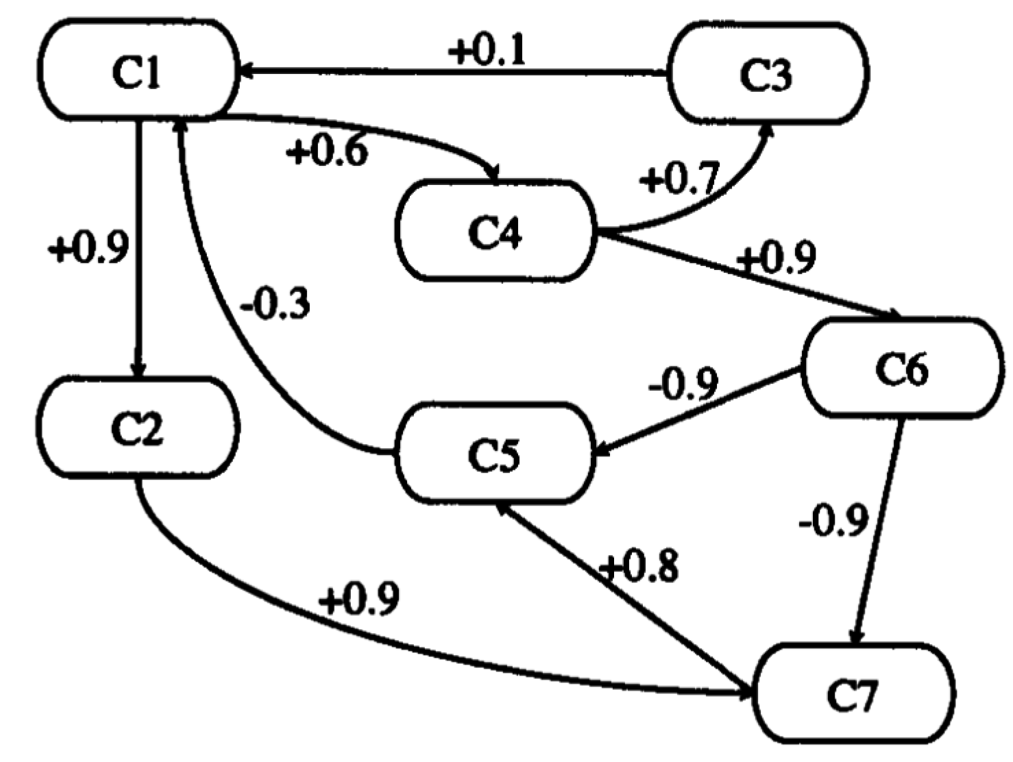
2.1. Fuzzy Cognitive Map (FCM)

A Fuzzy Cognitive Map F in Figure 1 shows a relationship system, which is a 4-tuple (C, W, A, f) mathematically, where

• C = {C₁,C₂,…,C_N} is a set of N concepts forming the nodes of a graph.
• W: (C_i,C_j)→w_ij is a function associating w_ij with a pair of concepts, with w_ij equal to the weight of edge directed from C_i to C_j, where w_ijϵ[−1, 1]. Thus, W(NN) is a connection matrix.

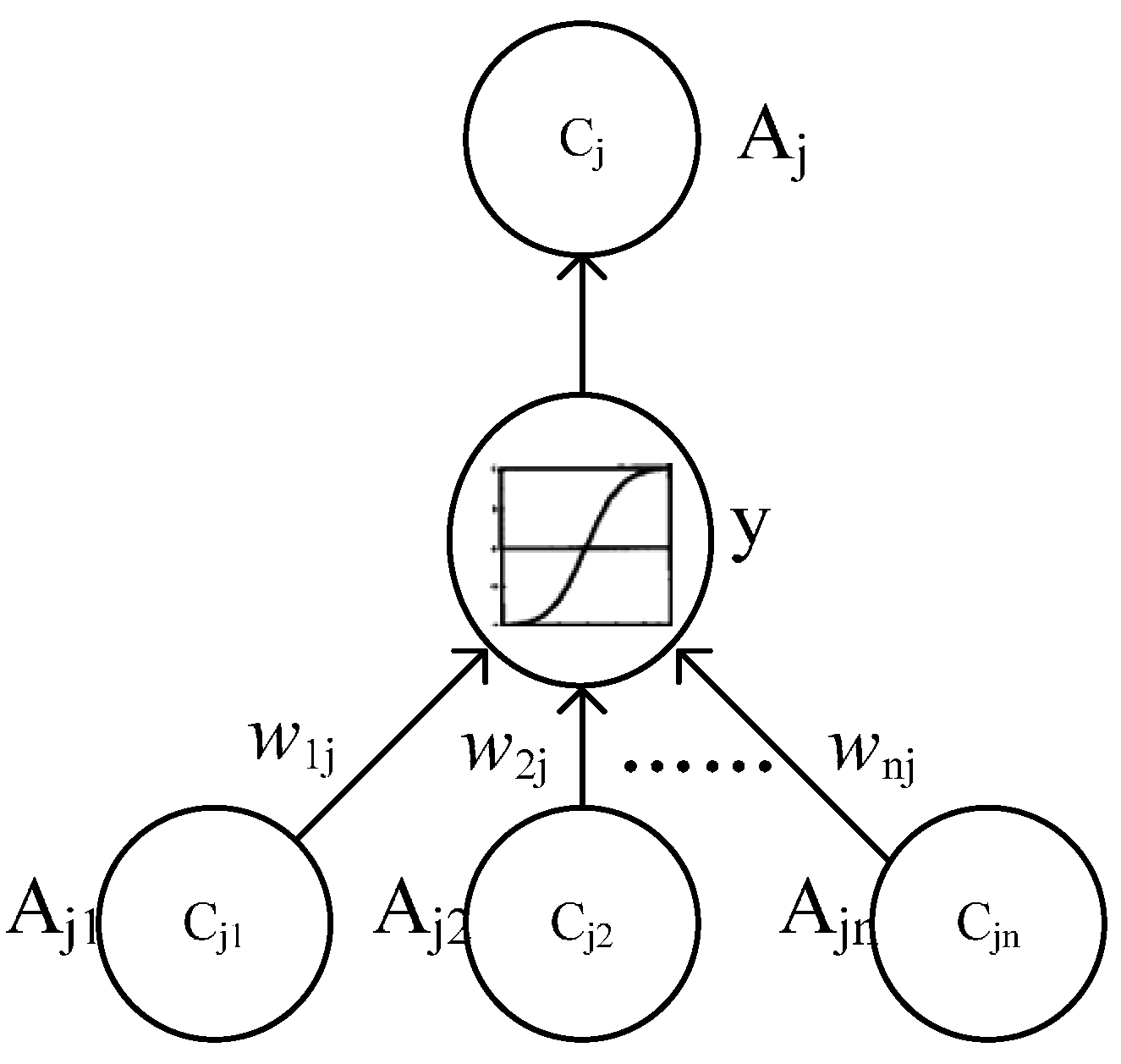
If there is positive causality between concepts C_i and C_j, then w_ij > 0, which means an increase of the value of concept C_i will cause an increase of the value of concept C_j and a decrease of the value of C_i will lead to a decrease of the value of C_j.

If there is inverse causality between the two concepts, then w_ij < 0, which represents an increase of the value of concept C_i will cause a decrease of the value of the second concept and a decrease of the value of concept C_i will cause an increase of the value of the concept C_j.

If there is no relationship between the two concepts, then w_ij = 0.

Figure 1. A simple fuzzy cognitive map.

Figure 1. A simple fuzzy cognitive map.

• A: C_i → A_i(t) is a function that associates each concept C_i with the sequence of its activation degrees such as for tϵT, A_i(t)ϵL given its activation degree at the moment t. A(0)ϵL^T indicates the initial vector and specifies initial values of all concept nodes and A(t)ϵL^T is a state vector at certain iteration t.
• f is a transformation or activation function, which includes recurring relationship on t ≥ 0 between A(t + 1) and A(t).

  $$A_j\left(t+1\right)=f(A_j\left(t\right)+{\displaystyle \sum }_{\begin{array}{c}i\ne j\\ i\in S\end{array}}{A}_i\left(t\right)w_{ij})$$

  (1)

The transformation function of FCM is with memory at previous moment shown as Equation (1), which is used to infer the state values of concepts in FCM. It limits the weighted sum to the range [0, 1] or [−1, 1]. The three most commonly used transformation (bivalent, trivalent, logistic) functions are shown below.

• Bivalent

  $$f\left(x\right)=\{\begin{array}{l}0,x\le 0\\ 1, x>0\end{array}$$
• Trivalent

  $$f\left(x\right)=\{\begin{array}{c}-1, x\le -0.5\\ 0, -0.5\le x\le 0.5\\ 1, x\ge 0.5\end{array}$$
• Logistic

  $$f\left(x\right)=\frac{1}{1+e^{-Cx}}$$

FCM can be used to perform simulation of an interconnected system. The vector A(t) in FCM specifies state values of all concepts (nodes) in the t iteration. An FCM has a number of successive state iterations. The state value of a concept is calculated by the preceding iteration of concepts states, which exert influence on the given node.

2.2. FCM Learning Algorithms

FCM learning algorithm is a kind of automated learning method to establish FCM model from data resources. There are two classes of FCM learning algorithms, Hebbian based learning and evolved based learning. The former are Hebbian based algorithms [14,15,16], mainly including NHL (Nonlinear Hebbian Learning), DD-NHL (Data-Driven Nonlinear Hebbian Learning) and AHL (Active Hebbian Learning). The differences of these algorithms are in the way of adjusting the edge weights. The latter are evolve based algorithms [17,18,19,20], which are composed of PSO (Particle Swarm Optimization), RCGA (Real Coded Genetic Algorithm), etc.

2.2.1. Nonlinear Hebbian Learning (NHL)

NHL is on the basis of the well-known Hebb’s learning law, which is a kind of unsupervised learning algorithm. Considering the nonlinear output unit, given random pre-synaptic an input vector x, weight vector w, and output z = f (w^T x). The nonlinear activation function f is a sigmoid function. The criterion function J maximized by Hebb’s rule may be written as Equation (2).

$$J=E[z^2]$$

(2)

An additional constraint such as ||w|| = 1 is necessary to stabilize the learning rule. A stochastic approximation solution is employed to the following nonlinear Hebbian learning rule as Equation (3).

$$\Delta w_{ji}={\mathsf{\eta }}_{k}z\frac{dz}{dy}(x_j-w_{ji}{y}_i)$$

(3)

Note that the nonlinear learning rules are seeking a set of weight parameters such that the outputs of the unit have the largest variance. The nonlinear unit constrains the output, ensuring it remains within a bounded range.

2.2.2. Real-Coded Genetic Algorithm (RCGA)

RCGA is a real-coded genetic algorithm to develop FCM connection matrix based on data resource. RCGA defines each chromosome as a floating-point vector. Each element in the vector is called gene. In case of the learning FCM with N node, each chromosome consists of N(N−1) genes, which are floating point numbers from the range [−1, 1], defined as follows.

E = [w₁₂, w₁₃, . . . , w_1N, w₂₁, w₂₃, . . . , w_2N, . . . , w_NN−1]^T

(4)

where w_ij is a weight value for an edge from i^th to j^th concept node. Each chromosome has to be decoded back into a candidate FCM. The number of chromosomes in a population is constant for each generation and it is specified by the population_size parameter.

The fitness function is calculated for each chromosome by computing the difference between system response generated using a FCM weights and a corresponding system response, which is known directly from the data resource. The difference is computed across all M−1 initial vector/system response pairs, and for the same initial state vector. The measure of error is shown as Equation (5).

$$Error\_L_p=\mathsf{\alpha }{\displaystyle \sum }_{t=1}^{M-1}{\displaystyle \sum }_{n=1}^N|A_n\left(t\right)-\widehat{A_n(t)}{|}^p$$

(5)

The parameter of $\mathsf{\alpha }$ is used to normalize error rate, and p is 1, 2 or $\mathsf{\infty }$. N is the number of concepts in FCM, and M is the number of iterations. The error measure can be used as the core of fitness function as Equation (6).

$$\text{Fitness function}=\frac{1}{a\times Error\_L_p+1}$$

(6)

The fitness function is normalized to the (0, 1]. The parameter $a$ can be set different value in different p condition.

The stopping condition of RCGA takes into consideration two possible scenarios of the learning process. One is the learning should be terminated when the fitness function value reaches a threshold value called max_fitness; the other is a maximum number of generations, named max_generation, has been reached. If the stopping conditions have not been reached, evolutionary operators and selection strategy need to be applied.

2.3. Problem Statements

In real world, a complex system has to have multi-dimensional groups with direct or indirect relationships, which generates multi-relational data. Moreover, each dimension maybe contains many concepts with different granularity relationships. For example, in a Mutagenesis system, there are three dimensions of atom, molecule and another atom, which are coarse-grained concepts; atype and charge are fine-grained concepts in the atom dimension; lumo, logp, indl and inda are fine-grained concepts in the molecule dimension. In two granularities, fine-grained concepts are on behalf of nodes in low-level and coarse-grained concepts represent hyper nodes. The coarse-grained concept of a dimension can be seen as a summary expression of its fine-grained concepts with multi-instances in low-level of the dimension.

Thus, problem to solve are: how to get summary evaluations in a dimension based on low-level data with multi-instances and how to mine high-level FCM from summary evaluations in dimensions for high-quality classification and causality.

3. Materials and Methods

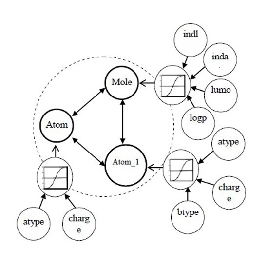
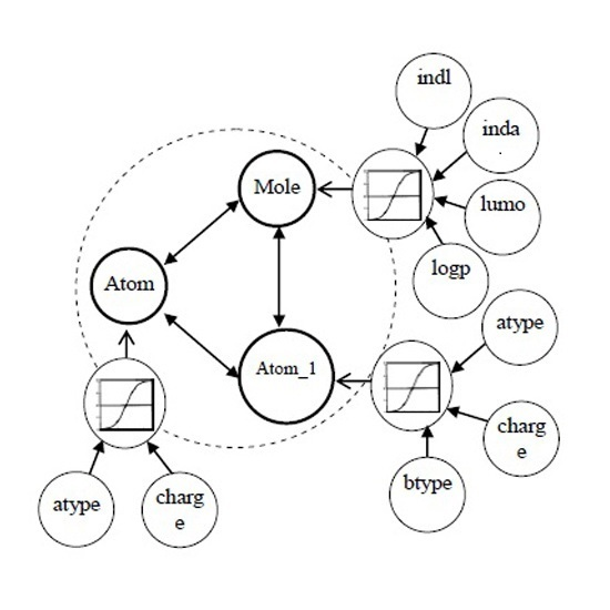
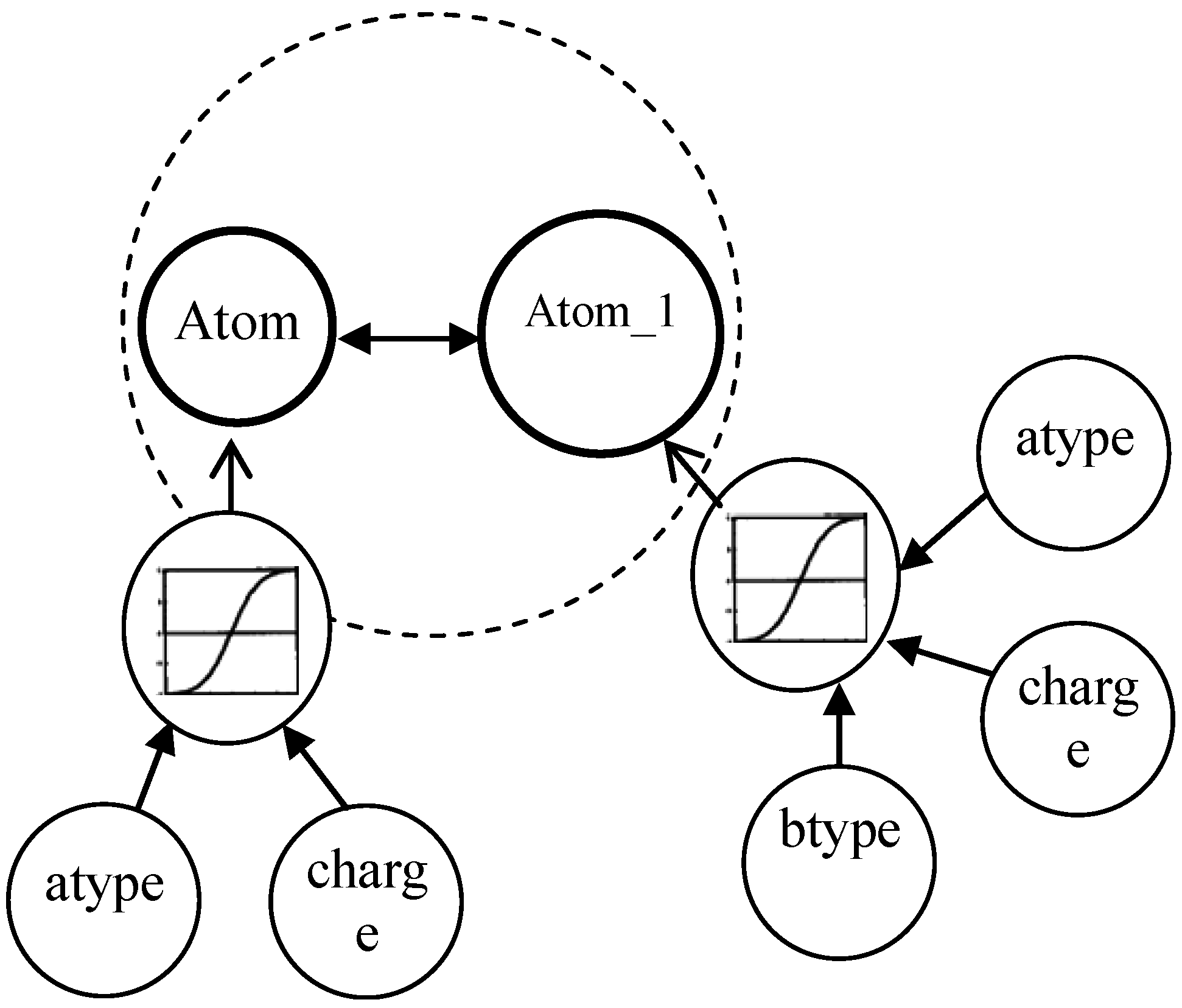
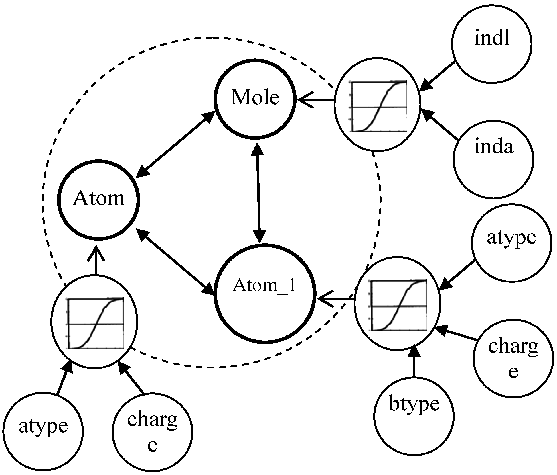
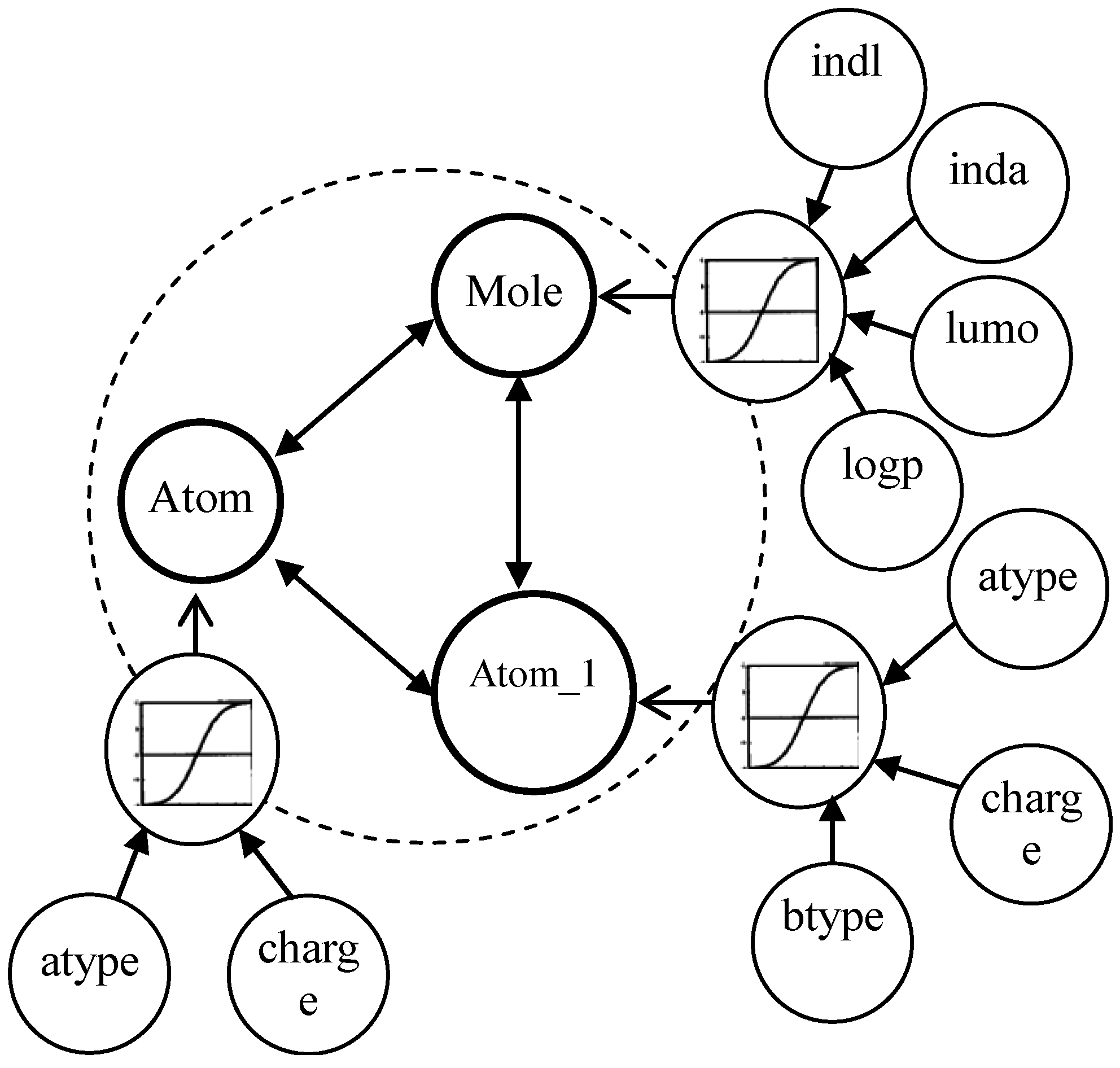
3.1. Multi-Relational FCM

In order to better model the multi-relationships and coarse-grained concepts in the complex system, undoubtedly, a multi-relational FCM (Definition 1), extended from FCM, can represent the multi-relationship system. The multi-relational FCM can be divided into different groups and different levels. A group means a dimension. A level is a granularity. Coarse-grained concepts are upper-level nodes. Fine-grained concepts are low-level nodes. A coarse-grained concept in a dimension represents a FCM composed of fine-grained concepts, and is related with other coarse-grained concepts in other dimensions.

Definition 1. 

A multi-relational FCM with two-levels and n-dimensions is U_n² = (C_n², W_n², A_n², f).

• C_n²: {{C_1i}…,{C_ji},…{C_ni}} is a set of concepts, {C_ji} is on behalf of a coarse-grained concept in j dimension, and C_ji is i^th fine-grained concept in bottom-level of j^th dimension.
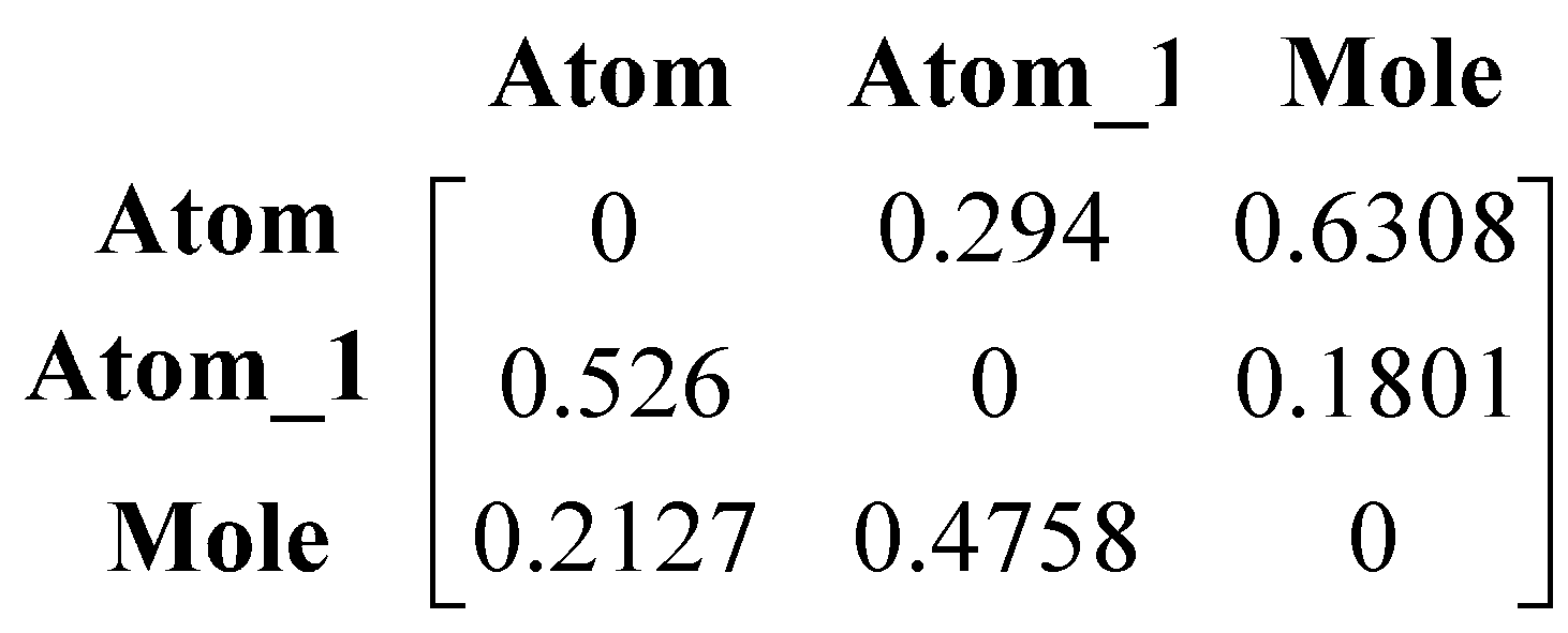
• W_n²: {{W_j}, {W_ij}}. <{C_ji}> → W_j is a function associating W_j among j^th dimension, W_j:{w_ij}; (<{C_1i}>…, <{C_ji}>,…<{C_ni}>) → {W_ij} is function associating between coarse-grained concepts.
• A_n²: C_ji → A_ji(t), {C_ji} → A_j(t). A_j(t) is a function f at iteration t.
• f is a transformation function, which includes recurring relationship on t ≥ 0 among A_j(t + 1), A_ji(t) and A_i(t), where A_j(0) is referred out based on the weight vector W_j, got by multi-instances oriented NHL, in low-level FCM.

3.2. Multi-Instances Oriented NHL

In the multi-relational FCM, each concept represents a useful field name in data resource. In the multi-relationship, one field in main table corresponding to another table has some sub fields. The field in the main table points to a coarse-grained concept in low-level FCM and the fields in another table indicate the fine-grained concepts in the FCM. Thus, the low-level FCM can be used to model the multi-relationship.

One coarse-grained concept (C_j) in j^th dimension corresponds to some fine-grained concepts (C_j1, C_j2, . . . , C_jn). It becomes the key to the state value of get the weights between the coarse-grained concept and some fine-grained concepts in the low-level FCM. The weights express the causality relationship between fine-gain concepts and coarse-grained concept. The weights need to be learned from multi-instances. NHL can be extended to multi-instances oriented mining for the optimistic of the nonlinear units’ weights in Figure 2. In the prerequisite, the state states of coarse-grained concepts in high-level FCM can be inferred.

Multi-instances oriented NHL has two constraints. First constraint is that it maximizes the mathematical expectation of $A_j^2$ of all multi-instances as Equation (7).

$$\mathrm{maxmize} J=E[{\displaystyle \sum }_r{A}_j^2]$$

(7)

$$\text{subject to }\left|\right|w\left|\right|=1$$

(8)

Figure 2. Nonlinear unit in Fuzzy Cognitive Map (FCM).

Figure 2. Nonlinear unit in Fuzzy Cognitive Map (FCM).

Second constraint is that the weight vector w has to be limited to stabilize the learning rule as Equation (8), which generates the following nonlinear Hebbian learning rule as Equation (9).

$$\Delta w_{ij}(t+1)=\mathsf{\eta }{A}_j(A_{ji}-w_{ij}(t)A_j)$$

(9)

Accordingly, multi-instances oriented NHL is presented in the function of M_NHL. The execution phase of multi-instances oriented NHL (M_NHL) is consisted of the following steps:

Step 1:

Random initialize the weight vector w_j(t), t = 0, p = 0 and input all instance {A_ji}

Step 2:

Calculate the mathematical expectation of A_j² of all {A_ji}

Step 3:

Set t = t + 1, repeat for each iteration step t:

3.1

Set p = p + 1, to the p^th instance:

3.1.1

Adjust w_j(t) matrix to {A_ji}^p by Equation (9)

3.2

Calculate the A_j² to all {A_ji} by Equation (10)

3.3

Determine whether A_j² is maximum or not at present

3.4

If A_j² is maximum, output the optimal w_j(t)

Step 4:

Return the final weight vector w_j(t)

According to the literature [21], whether NHL clusters better or not is closely related to the activation function f. It means that if cumulative normal distribution function or approximate cumulative logic distribution function is chosen as activation function, output results will show a U-distribution and easily achieve better NHL clustering. In order to avoid integral calculation, the cumulative logic distribution, shown as Equation (11), is selected. The output values (nonlinear unit outputs) can be inferred by Equation (10), where A_ij is the input and w_ji is mined by M_NHL algorithm.

$${\text{A}}_{\text{j}}(\text{t})=f({\displaystyle \sum }_{\text{i}\ne \text{j}}{A}_{ij}(\text{t}-1)w_{ji}(\text{t}-1))$$

(10)

$$f\left(x\right)=\frac{1-e^{-x}}{1+e^{-x}}$$

(11)

3.3. NHL and RCGA Based Integrated Algorithm

RCGA is used to get the weight matrix of high-level FCM for high-quality classification and causality based on initial state values of coarse-grained concepts, which are got by M_NHL in Section 3.2.

W = [W₁₂, W₁₃,…,W_1M,...,W_M1,…,W_M(M−1)]

(12)

Each chromosome consists of M(M−1) genes (see Equation (12)). M is the total number of hyper concepts or dimensions. The gene is a floating point number from the range [−1, 1]. W_ij specifies the weight between coarse-grained concept in i^th dimension and it in j^th dimension. Each chromosome can be decoded back into a high-level FCM.

When the fitness is more than max_fitness specified or the generation is more than max_generation specified, the procedure ends. The fitness function of RCGA is as follows (see Equation (13)).

$$fitness=\frac{1}{a{{\displaystyle \Sigma }}_{t=0}^T{{\displaystyle \Sigma }}_{j=1}^M{\left(A_j(t)-\widehat{A_j}\right)}^2+1}$$

(13)

where T is the number of iterations, $\widehat{A_j}$ is the actual output of j^th concept of system, A_j(t) is simulated output at t iteration by computing.

In the procedure, the algorithm needs to call function M_NHL. Moreover, if the fitness and the number of iterations are not satisfied with the max, the next chromosome is created by select method, mutation method and recombination method. In our experiments, a simple one-point crossover, random mutation and roulette wheel selection are applied. The parameters are chosen and set as Table 1.

Table 1. The parameters in the integrated algorithm.

Parameters	Values	Meanings
probability of recombination	0.9	probability of single-point crossover
probability of mutation	0.5	probability of random mutation
population_size	50	the number of chromosomes
max_generation	500,000	a maximum number of generations
max_fitness	[0.6, 0.9]	fitness thresholds
a	1000	a parameter in Equation (13)

Table 1. The parameters in the integrated algorithm.

Parameters	Values	Meanings
probability of recombination	0.9	probability of single-point crossover
probability of mutation	0.5	probability of random mutation
population_size	50	the number of chromosomes
max_generation	500,000	a maximum number of generations
max_fitness	[0.6, 0.9]	fitness thresholds
a	1000	a parameter in Equation (13)

The execution procedure of the algorithm integrating RCGA and NHL consisted of the following steps:

Step 1:

Initialize the parameters by the Table 1

Step 2:

Randomly initialize population_size chromosomes, g = 0, t = 0

Step 3:

Repeat for each dimension j:

3.1

Calculate A_j(t) by Equation (11) and w_j based on M_NHL

Step 4:

Repeat for each chromosome:

4.1

Calculate the fitness by A_j(t) and Equation (13)

Step 5:

Get max of the fitness and the W

Step 6:

if max of fitness not more than max_fitness and g not more than max_generation

6.1

Select chromosomes by roulette wheel selection

6.2

Recombination the chromosomes by single-point crossover

6.3

Random mutation to the chromosomes by the probability

6.4

Set t = i + 1, Repeat for each chromosome:

6.4.1

Calculate A_j(t) by Equation (1)

6.5

Set g = g + 1, go to Step 5

Step 7:

The W is the optimal chromosome.

The criterion in Equation (14) is defined as a normalized average error between corresponding concept values at each iteration between the two states. The error is used to define the accuracy of the algorithm simulating FCM.

$$error=\frac{1}{M\times T}{\displaystyle \sum }_{t=0}^T{\displaystyle \sum }_{j=1}^M|A_j(t)-{\widehat{A}}_j|$$

(14)

4. Results and Discussion

Experiments have been carried out using Mutagenesis describing molecular structure, which is a multi-relational dataset. The multi-relational system consists of five tables (relationships). They are Atom, Bond, Atom_1, Molatm and Mole, where Bond and Molatm play associations among other three tables. The class label is in Mole table. The Mutagenesis data describes 188 molecules falling in two classes, mutagenic (active) and non-mutagenic (inactive); 125 of these molecules are mutagenic.

A molecule is associated with multi-atoms through Molatm. An atom is associated with several atoms through Bond. So Mutagenesis can be expressed as a multi-relationship of three dimensions: Atom, Atom_1, and Mole. Each dimension has many fine-grained concepts, such as indl, inda, lumo, logp of molecular dimension.

There are three backgrounds of Mutagenesis shown in Table 2. The three multi-relational FCM structures as shown in Figure 3, Figure 4 and Figure 5 are different in three different backgrounds. The dotted lines show high-level FCMs.

Figure 3. FCM structure of Mutagenesis in BK₀.

Figure 3. FCM structure of Mutagenesis in BK₀.

Figure 4. FCM structure of Mutagenesis in BK₁.

Figure 4. FCM structure of Mutagenesis in BK₁.

Figure 5. FCM structure of Mutagenesis in BK₂.

Figure 5. FCM structure of Mutagenesis in BK₂.

Table 2. Three kinds of background of Mutagenesis.

Background	Description
BK0	Each compound includes the attributes of bond types, atom types, and partial charges on atoms
BK1	Each compound includes indl and inda of mole besides those in BK0
BK2	Each compound includes all attributes that are logp and lumo of mole besides those in BK1

Table 2. Three kinds of background of Mutagenesis.

Background	Description
BK0	Each compound includes the attributes of bond types, atom types, and partial charges on atoms
BK1	Each compound includes indl and inda of mole besides those in BK0
BK2	Each compound includes all attributes that are logp and lumo of mole besides those in BK1

The experiment is implemented for the class of molecular and the association weights among the three concepts (Atom, Atom_1 and Molecular) in the Mutagenesis.

For better operation efficiency in shorter runtime, an experiment, based on multi-relationship FCM and the integrated algorithm, has been carried out in the different fitness thresholds under three kinds of background. The learning runtimes are shown in the fitness thresholds from 0.6 to 0.9. From Figure 6, we can see that the changes of the runtime are not big under three kinds of background. The runtimes spent is changed. When the fitness threshold is at the interval of (0.65, 0.76], the operation takes less time.

Figure 6. The learning runtime under the different fitness thresholds.

Figure 6. The learning runtime under the different fitness thresholds.

The classification results are compared in the max_fitness = 0.7 under three backgrounds. From the Table 3, the classification runtime of the integrated method is longer. The main reason for this is the costs in database access and FCM inference. The integrated method has better classification accuracy according to the label in Mole in three kinds of background knowledge; in particular, the accuracy rate is best in BK₁.

Table 3. Classification efficiency in different backgrounds.

Backgrounds	Runtime(s)	Accuracy (%)
BK0	0.78	82.3%
BK1	0.8	82.9%
BK2	0.8	82.7%

Table 3. Classification efficiency in different backgrounds.

Backgrounds	Runtime(s)	Accuracy (%)
BK0	0.78	82.3%
BK1	0.8	82.9%
BK2	0.8	82.7%

And the method not only gets better classification, but also the association weights or causality for causal analysis of system, which is more than other methods. For example, the association matrix of high-level FCM of Mutagenesis in BK₂ is shown in Figure 7.

Figure 7. Association matrix of high-level FCM of Mutagenesis in BK₂.

Figure 7. Association matrix of high-level FCM of Mutagenesis in BK₂.

5. Conclusions

We construct a kind of multi-levels and multi-dimensions FCM to automatic model complex systems directly from multi-relational data resources. The multi-relational FCM include two levels and some dimensions. In the FCM, one concept in high-level has a summary evaluation in a dimension, which is inferred by the transformation function of low-level FCM. It has been solved that the weight vector in low-level FCM is learned by extended NHL from multi-instances for the inference. For getting better classification and causality, RCGA has been used in learning the association weights in high-level FCM. Moreover, the integrating algorithm of NHL and RCGA has been applied in the compounds of molecular of Mutagenesis, which obtains better accuracy and knowledge for causal analysis.

References

1. Han, J.W.; Kamber, M. Concept and Technology of Data Mining; Machinery Industry Press: Beijing, China, 2007; pp. 373–383. [Google Scholar]
2. Spyropoulou, E.; de Bie, T.; Boley, M. Interesting pattern mining in multi-relational data. Data Knowl. Eng. 2014, 28, 808–849. [Google Scholar] [CrossRef]
3. Yin, X.; Han, J.; Yang, J.; Yu, P.S. Efficient classification across multiple database relations: A CrossMine approach. IEEE Trans. Knowl. Data Eng. 2006, 18, 770–783. [Google Scholar] [CrossRef]
4. Xu, G.; Yang, B.; Qin, Y.; Zhang, W. Multi-relational Naive Bayesian classifier based on mutual information. J. Univ. Sci. Technol. Beijing 2008, 30, 943–966. [Google Scholar]
5. Liu, H.; Yin, X.; Han, J. An efficient multi-relational naive Bayesian classifier based on semantic relationship graphs. In Proceedings of the 2005 ACM-SIGKDD Workshop on Multi-Relational Data Mining (KDD/MRDM05), Chicago, IL, USA, 21–24 August 2005.
6. Kosko, B. Fuzzy cognitive maps. Int. J. Man Mach. Studs. 1986, 24, 65–75. [Google Scholar] [CrossRef]
7. Papageorgiou, E.I.; Salmeron, J.L. A review of fuzzy cognitive maps research during the last decade. IEEE Trans. Fuzzy Syst. 2013, 12, 66–79. [Google Scholar] [CrossRef]
8. Groumpos, P.P. Large scale systems and fuzzy cognitive maps: A critical overview of challenges and research opportunities. Annu. Rev. Control 2014, 38, 93–102. [Google Scholar] [CrossRef]
9. Zhang, Y. Modeling and Control of Dynamic Systems Based on Fuzzy Cognitive Maps. Ph.D. Thesis, Dalian University of Technology, Dalian, China, 2012. [Google Scholar]
10. Mago, V.K.; Bakker, L.; Papageorgiou, E.I.; Alimadad, A.; Borwein, P.; Dabbaghian, V. Fuzzy cognitive maps and cellular automata: An evolutionary approach for social systems modeling. Appl. Soft Comput. 2012, 12, 3771–3784. [Google Scholar] [CrossRef]
11. Subramanian, J.; Karmegam, A.; Papageorgiou, E.; Papandrianos, N.I.; Vasukie, A. An integrated breast cancer risk assessment and management model based on fuzzy cognitive maps. Comput. Methods Programs Biomed. 2015, 118, 280–297. [Google Scholar] [CrossRef] [PubMed]
12. Szwed, P.; Skrzynski, P. A new lightweight method for security risk assessment based on fuzzy cognitive maps. Appl. Math. Comput. Sci. 2014, 24, 213–225. [Google Scholar] [CrossRef]
13. Peng, Z.; Peng, J.; Zhao, W.; Chen, Z. Research on FCM and NHL based High Order mining driven by big data. Math. Probl. Eng. 2015, 2015. [Google Scholar] [CrossRef]
14. Papakostas, G.A.; Koulouriotis, D.E.; Polydoros, A.S.; Tourassis, V.D. Towards Hebbian learning of fuzzy cognitive maps in pattern classification problems. Expert Syst. Appl. 2012, 39, 10620–10629. [Google Scholar] [CrossRef]
15. Salmeron, J.L.; Papageorgiou, E.I. Fuzzy grey cognitive maps and nonlinear Hebbian learning in process control. Appl. Intell. 2014, 41, 223–234. [Google Scholar] [CrossRef]
16. Beena, P.; Ganguli, R. Structural damage detection using fuzzy cognitive maps and Hebbian learning. Appl. Soft Comput. 2011, 11, 1014–1020. [Google Scholar] [CrossRef]
17. Kim, M.-C.; Kim, C.O.; Hong, S.R.; Kwon, I.-H. Forward-backward analysis of RFID-enabled supply chain using fuzzy cognitive map and genetic algorithm. Expert Syst. Appl. 2008, 35, 1166–1176. [Google Scholar] [CrossRef]
18. Froelich, W.; Papageorgiou, E.I. Extended evolutionary learning of fuzzy cognitive maps for the prediction of multivariate time-series. Fuzzy Cogn. Maps Appl. Sci. Eng. 2014, 2014, 121–131. [Google Scholar]
19. Froelich, W.; Salmeron, J.L. Evolutionary learning of fuzzy grey cognitive maps for forecasting of multivariate, interval-valued time series. Int. J. Approx. Reason. 2014, 55, 1319–1335. [Google Scholar] [CrossRef]
20. Wojciech, S.; Lukasz, K.; Witold, P. A divide and conquer method for learning large fuzzy cognitive maps. Fuzzy Sets Syst. 2010, 161, 2515–2532. [Google Scholar]
21. Sudjianto, A.; Hassoun, M.H. Statistical basis of nonlinear Hebbian learning and application to clustering. Neural Netw. 1995, 8, 707–715. [Google Scholar] [CrossRef]