The Noise Blowing-Up Strategy Creates High Quality High Resolution Adversarial Images against Convolutional Neural Networks

Abstract

Convolutional neural networks (CNNs) serve as powerful tools in computer vision tasks with extensive applications in daily life. However, they are susceptible to adversarial attacks. Still, attacks can be positive for at least two reasons. Firstly, revealing CNNs vulnerabilities prompts efforts to enhance their robustness. Secondly, adversarial images can also be employed to preserve privacy-sensitive information from CNN-based threat models aiming to extract such data from images. For such applications, the construction of high-resolution adversarial images is mandatory in practice. This paper firstly quantifies the speed, adversity, and visual quality challenges involved in the effective construction of high-resolution adversarial images, secondly provides the operational design of a new strategy, called here the noise blowing-up strategy, working for any attack, any scenario, any CNN, any clean image, thirdly validates the strategy via an extensive series of experiments. We performed experiments with 100 high-resolution clean images, exposing them to seven different attacks against 10 CNNs. Our method achieved an overall average success rate of 75% in the targeted scenario and 64% in the untargeted scenario. We revisited the failed cases: a slight modification of our method led to success rates larger than 98.9%. As of today, the noise blowing-up strategy is the first generic approach that successfully solves all three speed, adversity, and visual quality challenges, and therefore effectively constructs high-resolution adversarial images with high-quality requirements.

1. Introduction

The ability of convolutional neural networks (CNNs) [1] to automatically learn from data has made them a powerful tool in a wide range of applications touching on various aspects of our daily lives, such as image classification [2,3], object detection [4], facial recognition [5], autonomous vehicles [6], medical image analysis [7,8], natural language processing (NLP) [9,10], augmented reality (AR) [11], quality control in manufacturing [12] and satellite image analysis [13,14].

Even so, CNNs are vulnerable to attacks. In the context of image classification, which is considered in the present paper, carefully designed adversarial noise added to the original image can lead to adversarial images being misclassified by CNNs. These issues can lead to serious safety problems in real-life applications. On the flip side, such vulnerabilities can be also leveraged to obscure security and privacy-sensitive information from CNN-based threat models seeking to extract such data from images [15,16,17].

In a nutshell, adversarial attacks are categorized based on two components: the level of knowledge the attacker has about the CNN; the scenario followed by the attack. Regarding the first component, in a white-box attack [3,18,19,20,21] (also known as gradient-based attack), the attacker has full access to the architecture and to the parameters of the CNN. In contrast, in a black box attack [22,23,24,25,26,27], the attacker does not know the CNN’s parameters or architecture; its knowledge is limited to the CNN’s evaluation for any input image, including the label category in which it classifies the image, and the corresponding label value. As a consequence of the knowledge bias, white-box attacks usually generate adversarial images faster than black-box attacks. Regarding the second component, in the target scenario, the goal of the attack is to manipulate the clean input image to create an adversarial image that the CNN classifies into a predefined target category. In the untargeted scenario, the goal of the attack is to create an adversarial image that the CNN classifies into any category other than the category of the clean image. An additional objective in these scenarios is to require that the modifications put on the original clean image to create the adversarial image remain imperceptible to a human eye.

1.1. Standart Adversarial Attacks

To perform image recognition, CNNs start their assessment of any image by first resizing it to its own input size. In particular, high-resolution images are scaled down, say to $32\times 32$ or $224\times 244$ for most CNNs trained on CIFAR-10, respectively on ImageNet [28]. Until recently (and still now), to the best of our knowledge, attacks are performed on these resized images. Consequently, the resulting adversarial images’ size coincides with the CNN input’s size, regardless of the size of the original images. Figure 1 describes this standard approach, in which attacks take place in the low-resolution domain, denoted as the $\mathcal{R}$ domain in this paper.

Figure 1. Standard attacks’ process, where $c_a$ is the CNN’s leading category of the clean resized image, and $c\ne c_a$ is the CNN’s leading category of the adversarial image.

As previously highlighted, the susceptibility of CNNs to adversarial attacks can be utilized to obfuscate privacy-sensitive information from CNN-empowered malicious software. To use adversarial images for such security purposes, their sizes must match the sizes of the original clean images considered. In practice, these sizes are usually far larger than $224\times 224$. However, generating high-resolution adversarial images, namely adversarial images in the $\mathcal{H}$ domain as we call it in this paper, poses certain difficulties.

1.2. Challenges and Related Works

Creating adversarial images of the same size as their clean counterparts, as illustrated in Figure 2, is a novel and highly challenging task in termes of speed, adversity, and imperceptibility.

Figure 2. Direct attack process generating an adversarial image with the same size as the original clean image.

Firstly, the complexity of the problem grows quadratically with the size of the images. This issue impacts the speed of attacks performed directly in the $\mathcal{H}$ domain. In [29], an evolutionary algorithm-based black-box attack, that successfully handled images of sizes $224\times 224$, was tested on a high-resolution image of size $910\times 607$ via the direct approach illustrated in Figure 2. Despite 40 h of computational efforts, it failed to create a high-resolution adversarial image by this direct method. This indicates that a direct attack in the $\mathcal{H}$ domain, as described above, is unlikely to succeed. An alternative approach is definitively needed to speed up the attack process in the $\mathcal{H}$ domain.

Additionally, the adversarial noise in the high-resolution adversarial image should prevail even when the adversarial image is resized to the input size of the CNN. Finally, the difference between the high-resolution original clean image and the high-resolution adversarial image must be imperceptible to a human eye.

A first solution to the speed and adversity challenges is presented in [29,30] as an effective strategy that smoothly transforms an adversarial image — regardless of how it is generated—from the $\mathcal{R}$ domain to the $\mathcal{H}$ domain. However, the imperceptibility issue was not resolved.

1.3. Our Contribution

In this article, we introduce a novel strategy, extending our conference paper [31] (and enhancing [29,30]). This strategy stands as the first effective method for generating high visual quality adversarial images in the high-resolution domain in the following sense: The strategy works for any attack, any scenario, any CNN, and any clean high-resolution image. Compared to related works, our refined strategy increases substantially the visual quality of the high-resolution adversarial images, as well as the speed and efficiency in creating them. In summary, the approach amounts to a “blowing-up” to the high-resolution domain of the adversarial noise—only of the adversarial noise, and not of the full adversarial image—created in the low-resolution domain. Adding this high-resolution noise to the original high-resolution clean image leads to an indistinguishable high-resolution adversarial image.

This noise blowing-up strategy is validated in terms of speed, adversity, and visual quality by an extensive set of experiments. It encompasses seven attacks (four white-box and three black-box) against 10 state-of-the-art CNNs trained on ImageNet; the attacks are performed both for the untargeted and the target scenario, with 100 high-resolution clean images. In particular, the visual quality of high-resolution adversarial images generated with our method is thoroughly studied; the outcomes are compared with adversarial images resulting from [29,30].

1.4. Organisation of the Paper

Our paper is organised as follows. Section 2 recalls briefly what are the target and untarget scenarios in $\mathcal{R}$, what their versions in $\mathcal{H}$, fixes some notations, and lists a series of indicators ($L_p$ norms and FID) used to assess the human perception of distinct images. Section 3 formalises the noise blowing-up strategy, provides the scheme of the attack $at{k}_{\mathcal{H},\mathcal{C}}$ that lifts to $\mathcal{H}$ any attack $at{k}_{\mathcal{R},\mathcal{C}}$ against a CNN $\mathcal{C}$ that works in the $\mathcal{R}$ domain, and that takes advantage of lifting the adversarial noise only. It recalls some complementary indicators used to assess the impact of the obtained tentative adversarial images (Loss function ${\mathcal{L}}_{\mathcal{C}}$, “safety buffer” ${\Delta }_{\mathcal{C}}$), and again fixes some notations. The experimental study is performed in the subsequent Sections. Section 4 describes the ingredients of the experiments: the resizing functions, the 10 CNNs, the 100 clean high-resolution images, the target categories considered in the target scenario, and the 7 attacks. Section 5 provides the results of the experiments performed under these conditions: success rate, visual quality, and imperceptibility of the difference between adversarial and clean images, timing, and overhead of the noise blowing-up strategy. The cases, where the standard implementation of the strategy failed to succeed, are revisited in Section 6 thanks to the “safety buffer” ${\Delta }_{\mathcal{C}}$. Finally, Section 7 provides a comparison of the noise blowing-up method with the generic lifting method [29,30] on three challenging high-resolution images, one CNN, and one attack for the target scenario. Section 8 summarizes our findings, and indicates directions for future research. An Appendix completes the paper with additional data and evidence.

All algorithms and experiments were implemented using Python 3.9 [32] with NumPy 1.23.5 [33], TensorFlow 2.14.0 [34], Keras 3 [35], and Scikit 0.22 [36] libraries. Computations were performed on nodes with Nvidia Tesla V100 GPGPUs of the IRIS HPC Cluster at the University of Luxembourg.

2. CNNs and Attack Scenarios

CNNs performing image classification are trained on some large dataset $\mathcal{S}$ to sort images into predefined categories $c_1,\cdots ,c_{\ell }$. The categories, and their number ℓ, are associated with $\mathcal{S}$ and are common to all CNNs trained on $\mathcal{S}$. One denotes $\mathcal{R}$ the set of images of size $r_1\times r_2$ (where $r_1$ is the height, and $r_2$ is the width of the image) natively adapted to such CNNs.

Once trained, a CNN can be exposed to images (typically) in the same domain $\mathcal{R}$ as those on which it was trained. Given an input image $\mathcal{I}\in \mathcal{R}$, the trained CNN produces a classification output vector

$${\mathbf{o}}_{\mathcal{I}}=\left({\mathbf{o}}_{\mathcal{I}}\left[1\right],\cdots ,{\mathbf{o}}_{\mathcal{I}}[\ell ]\right),$$

(1)

where $0\le {\mathbf{o}}_{\mathcal{I}}\left[i\right]\le 1$ for $1\le i\le \ell$, and ${\sum }_{i=1}^{\ell }{\mathbf{o}}_{\mathcal{I}}\left[i\right]=1$. Each $c_i$-label value ${\mathbf{o}}_{\mathcal{I}}\left[i\right]$ measures the plausibility that the image $\mathcal{I}$ belongs to the category $c_i$.

Consequently, the CNN classifies the image $\mathcal{I}$ as belonging to the category $c_k$ if $k={arg\; max}_{1\le i\le \ell }\left({\mathbf{o}}_{\mathcal{I}}\left[i\right]\right)$. If there is no ambiguity on the dominating category (as occurs for most images used in practice; we also make this assumption in this paper), one denotes $(c_k,{\mathbf{o}}_{\mathcal{I}}\left[k\right])$ the pair specifying the dominating category and the corresponding label value. The higher the $c_k$-label value ${\mathbf{o}}_{\mathcal{I}}\left[k\right]$, the higher the confidence that $\mathcal{I}$ represents an object of the category $c_k$ from CNN’s “viewpoint”. For the sake of simplicity and consistency with the remaining of this paper, we shall write $(c_{\mathcal{I}},{\tau }_{c_{\mathcal{I}}})=(c_k,{\mathbf{o}}_{\mathcal{I}}\left[k\right])$. In other words, $\mathcal{C}$’s classification of $\mathcal{I}$ is

$$\mathcal{C}\left(\mathcal{I}\right)=(c_{\mathcal{I}},{\tau }_{c_{\mathcal{I}}})\in \mathcal{V}=\{(c_i,v_i),\mathrm{where}{v}_i\in [0,1]\mathrm{for}1\le i\le \ell \}.$$

(2)

2.1. Assessment of the Human Perception of Distinct Images

Given two images $\mathcal{A}$ and $\mathcal{B}$ of the same size $h\times w$ (belonging or not to the $\mathcal{R}$ domain), there are different ways to assess numerically the human perception of the difference between them, as well as the actual “weight” of this difference. In the present study, this assessment is performed mainly by computing the (normalized) values of $L_p(\mathcal{A},\mathcal{B})$ for $p=0,1,2$, or ∞ and the Fréchet Inception Distance (FID).

Introduced in [37], FID originally served as a metric to evaluate the performance of GANs by assessing the similarity of generated images. FID is one of the recent tools for assessing the visual quality of adversarial images and it aligns closely with human judgment (see [38,39,40]). On the other hand, [41,42] provide an assessment of $L_p$-norms as a measure of perceptual distance between images.

In a nutshell, for an image $\mathcal{I}$ of size $h\times w$, the integer

$$0\le p_{i,j,\alpha }\left(\mathcal{I}\right)\le 255$$

denotes the value of the pixel positioned in the ith-row, jth-column, of the image $\mathcal{I}$ for the channel $\alpha \in \{R,G,B\}$ (R = Red, G = Green, B = Blue). Then,

• $L_0^{norm}(\mathcal{A},\mathcal{B})=\frac{1}{3hw}\#\{i,j,\alpha ;p_{i,j,\alpha }\left(\mathcal{A}\right)\ne p_{i,j,\alpha }\left(\mathcal{B}\right)\}$,
• $L_1^{norm}(\mathcal{A},\mathcal{B})=\frac{1}{2^{8}3hw}{\sum }_{i,j,\alpha }|p_{i,j,\alpha }\left(\mathcal{A}\right)-p_{i,j,\alpha }\left(\mathcal{B}\right)|$,
• $L_2^{norm}(\mathcal{A},\mathcal{B})=\frac{1}{2^{8}3hw}\sqrt{{\sum }_{i,j,\alpha }{|p_{i,j,\alpha }\left(\mathcal{A}\right)-p_{i,j,\alpha }\left(\mathcal{B}\right)|}^2}$,
• $L_{\infty }(\mathcal{A},\mathcal{B})={\mathrm{Max}}_{i,j,\alpha }|p_{i,j,\alpha }\left(\mathcal{A}\right)-p_{i,j,\alpha }\left(\mathcal{B}\right)|$

where $1\le i\le h,1\le j\le w$, and $\alpha \in \{R,G,B\}$. These quantities satisfy the inequalities:

$$0\le L_0^{norm}(\mathcal{A},\mathcal{B}),L_1^{norm}(\mathcal{A},\mathcal{B}),L_2^{norm}(\mathcal{A},\mathcal{B})\le 1,\mathrm{and}0\le L_{\infty }(\mathcal{A},\mathcal{B})\le 256.$$

The closer their values are to 0, the closer are the images $\mathcal{A},\mathcal{B}$ to each other.

To effectively capture the degree of disturbance, and therefore to provide a reliable measure of the level of disruption, FID quantifies the separation between clean and disturbed images based on extracting features from images that are provided by the Inception-v3 network [43]. Activations from one of the intermediate layers of the Inception v3 model are used as feature representations for each image. FID assesses the similarity between two probability distributions in a metric space, via the formula:

• FID($\mathcal{A}$, $\mathcal{B}$) $={\parallel {\mu }_{\mathcal{A}}-{\mu }_{\mathcal{B}}\parallel }^2+\mathrm{Tr}(M_{\mathcal{A}}+M_{\mathcal{B}}-2·\sqrt{M_{\mathcal{A}}·M_{\mathcal{B}}})$

where, ${\mu }_{\mathcal{A}}$ and ${\mu }_{\mathcal{B}}$ denote feature-wise mean vectors for the images $\mathcal{A}$ and $\mathcal{B}$, respectively, reflecting average features observed across the images. $M_{\mathcal{A}}$ and $M_{\mathcal{B}}$ represent covariance matrices for the feature vectors (covariance matrices offer insights into how features in the vectors co-vary with each other). The quantity ${\parallel {\mu }_{\mathcal{A}}-{\mu }_{\mathcal{B}}\parallel }^2$ captures the squared difference in mean vectors (highlighting disparities in these average features), and the trace quantity assesses dissimilarities between the covariance matrices. In the end, FID quantifies how similar the distribution of feature vectors in the $\mathcal{A}$ is to that in the $\mathcal{B}$. The lower the FID value, the more similar the images $\mathcal{A}$ and $\mathcal{B}$.

2.2. Attack Scenarios in the $\mathcal{R}$ Domain

Let $\mathcal{C}$ be a trained CNN, $c_a$ be a category among the ℓ possible categories, and $\mathcal{A}$ a clean image in the $\mathcal{R}$ domain, classified by $\mathcal{C}$ as belonging to $c_a$. Let ${\tau }_a$ be its $c_a$-label value. Based on these initial conditions, we describe two attack scenarios (the target scenario and the untarget scenario) aiming at creating an adversarial image $\mathcal{D}\in \mathcal{R}$ accordingly.

Whatever the scenario, one requires that $\mathcal{D}$ remains so close to $\mathcal{A}$, that a human would not notice any difference between $\mathcal{A}$ and $\mathcal{D}$. This is done in practice by fixing the value of the parameter $ϵ$, which controls (or restricts) the global maximum amplitude allowed for the modifications of each pixel value of $\mathcal{A}$ to construct an adversarial image $\mathcal{D}$. Note that, for a given attack scenario, the value set to $ϵ$ usually depends on the concrete performed attack, more specifically on the $L_p$ distance used in the attack to assess the human perception between an original and an adversarial image.

The $(c_a,c_t)$target scenario performed on $\mathcal{A}$ requires first to select a category $c_t\ne c_a$. The attack then aims at constructing an image $\mathcal{D}$ that is either a good enough adversarial image or a $\tau$-strong adversarial image.

A good enough adversarial image is an adversarial image that $\mathcal{C}$ classifies as belonging to the target category $c_t$, without any requirement on the $c_t$-label value ${\tau }_t$ beyond being strictly dominant among all label values. A $\tau$-strong adversarial image is an adversarial image that $\mathcal{C}$ not only classifies as belonging to the target category $c_t$, but for which its $c_t$-label value ${\tau }_t\ge \tau$ for some threshold value $\tau \in [0,1]$ fixed a priori.

In the untarget scenario performed on $\mathcal{A}$, the attack aims at constructing an image $\mathcal{D}$ that $\mathcal{C}$ classifies in any category $c\ne c_a$.

One writes $at{k}_{\mathcal{R},\mathcal{C}}^{scenario}$ to denote the specific attack atk performed to deceive $\mathcal{C}$ in the $\mathcal{R}$ domain according to the selected scenario, and $\mathcal{D}=at{k}_{\mathcal{R},\mathcal{C}}^{scenario}\left(\mathcal{A}\right)$ an adversarial image obtained by running successfully this attack on the clean image $\mathcal{A}$. Note that one usually considers only the first adversarial image obtained by a successful run of an attack, so that $\mathcal{D}$ is uniquely defined.

Finally, one writes $\mathcal{C}\left(\mathcal{D}\right)=(c,{\tau }_c)$ the classification of the adversarial image obtained. Note that $(c,{\tau }_c)=(c_t,{\tau }_t)$ in the case of the target scenario.

2.3. Attack Scenarios Expressed in the $\mathcal{H}$ Domain

In the context of high-resolution (HR) images, let us denote by $\mathcal{H}$ the set of images that are larger than those of $\mathcal{R}$. In other words, an image of size $h\times w$ (where h designates the height, and w the width of the image considered) belongs to $\mathcal{H}$ if $h\ge r_1$ and $w\ge r_2$. One assumes given a fixed degradation function

$$\rho : \mathcal{H}⟶\mathcal{R},$$

(3)

that transforms any image $\mathcal{I}\in \mathcal{H}$ into a “degraded” image $\rho \left(\mathcal{I}\right)\in \mathcal{R}$. Then there is a well-defined composition of maps $\mathcal{C}\circ \rho$ as shown in the following scheme:

(4)

Given ${\mathcal{A}}_a^{\mathrm{hr}}\in \mathcal{H}$, one obtains that way the classification of the reduced image ${\mathcal{A}}_a=\rho \left({\mathcal{A}}_a^{\mathrm{hr}}\right)\in \mathcal{R}$ as $\mathcal{C}\left({\mathcal{A}}_a\right)\in \mathcal{V}$.

We assume that the dominating category of the reduced image ${\mathcal{A}}_a$ is without ambiguity, and denote by $\mathcal{C}\left({\mathcal{A}}_a\right)=(c_a,{\tau }_a)\in \mathcal{V}$ the outcome of $\mathcal{C}$’s classification of ${\mathcal{A}}_a$.

Thanks to the degradation function $\rho$, one can express in the $\mathcal{H}$ domain any attack scenario that makes sense in the $\mathcal{R}$ domain. This is in particular the case for the target scenario and for the untarget scenario.

Indeed, an adversarial HR image against $\mathcal{C}$ for the $(c_a,c_t)$target scenario performed by an attack $at{k}_{\mathcal{H},\mathcal{C}}^{target}$ on ${\mathcal{A}}_a^{\mathrm{hr}}\in \mathcal{H}$ is an image ${\mathcal{D}}_t^{\mathrm{hr},\mathcal{C}}\left({\mathcal{A}}_a^{\mathrm{hr}}\right)=at{k}_{\mathcal{H},\mathcal{C}}^{target}\left({\mathcal{A}}_a^{\mathrm{hr}}\right)\in \mathcal{H}$, that satisfies two conditions (note that the notation ${\mathcal{D}}_t^{\mathrm{hr},\mathcal{C}}\left({\mathcal{A}}_a^{\mathrm{hr}}\right)$, with t as index, encapsulates and summarizes the fact that the adversarial image is obtained for the specific target scenario considered). On the one hand, a human should not be able to notice any visual difference between the original ${\mathcal{A}}_a^{\mathrm{hr}}$ and the adversarial ${\mathcal{D}}_t^{\mathrm{hr},\mathcal{C}}\left({\mathcal{A}}_a^{\mathrm{hr}}\right)$ HR images. On the other hand, $\mathcal{C}$ should classify the degraded image ${\mathcal{D}}_t^{\mathcal{C}}\left({\mathcal{A}}_a^{\mathrm{hr}}\right)=\rho \left({\mathcal{D}}_t^{\mathrm{hr},\mathcal{C}}\left({\mathcal{A}}_a^{\mathrm{hr}}\right)\right)$ in the category $c_t$ for a sufficiently convincing $c_t$-label value. The image ${\mathcal{D}}_t^{\mathrm{hr},\mathcal{C}}\left({\mathcal{A}}_a^{\mathrm{hr}}\right)\in \mathcal{H}$ is then a good enough adversarial image or a $\tau$-strong adversarial image if its reduced version ${\mathcal{D}}_t^{\mathcal{C}}\left({\mathcal{A}}_a^{\mathrm{hr}}\right)=\rho \left({\mathcal{D}}_t^{\mathrm{hr},\mathcal{C}}\left({\mathcal{A}}_a^{\mathrm{hr}}\right)\right)$ is.

Similarly, and mutatis mutandis for the untarget scenario, one denotes by ${\mathcal{D}}_{\mathrm{untarget}}^{\mathrm{hr},\mathcal{C}}\left({\mathcal{A}}_a^{\mathrm{hr}}\right)=at{k}_{\mathcal{H},\mathcal{C}}^{untarget}\left({\mathcal{A}}_a^{\mathrm{hr}}\right)$ the HR adversarial images obtained by an attack $at{k}_{\mathcal{H},\mathcal{C}}^{untarget}$ for the untarget scenario performed on ${\mathcal{A}}_a^{\mathrm{hr}}\in \mathcal{H}$, and by ${\mathcal{D}}_{\mathrm{untarget}}^{\mathcal{C}}\left({\mathcal{A}}_a^{\mathrm{hr}}\right)\in \mathcal{R}$ its degraded version.

The generic attack scenario on $\mathcal{C}$ in the HR domain can be visualized in the following scheme:

(5)

Depending on the scenario considered, one has:

• For the target scenario: ${\mathcal{D}}_{scenario}^{\mathrm{hr},\mathcal{C}}\left({\mathcal{A}}_a^{\mathrm{hr}}\right)={\mathcal{D}}_t^{\mathrm{hr},\mathcal{C}}\left({\mathcal{A}}_a^{\mathrm{hr}}\right)=at{k}_{\mathcal{H},\mathcal{C}}^{target}\left({\mathcal{A}}_a^{\mathrm{hr}}\right)\in \mathcal{H}$, ${\mathcal{D}}_{scenario}^{\mathcal{C}}\left({\mathcal{A}}_a^{\mathrm{hr}}\right)={\mathcal{D}}_t^{\mathcal{C}}\left({\mathcal{A}}_a^{\mathrm{hr}}\right)=\rho \left({\mathcal{D}}_t^{\mathrm{hr},\mathcal{C}}\left({\mathcal{A}}_a^{\mathrm{hr}}\right)\right)\in \mathcal{R}$, and $(c,{\tau }_c)=(c_t,{\tau }_t)$ with $c_t$ dominant among all categories, and, furthermore, ${\tau }_t\ge \tau$ if one additionally requires the adversarial image to be $\tau$-strong adversarial.
• For the untarget scenario: ${\mathcal{D}}_{scenario}^{\mathrm{hr},\mathcal{C}}\left({\mathcal{A}}_a^{\mathrm{hr}}\right)={\mathcal{D}}_{\mathrm{untarget}}^{\mathrm{hr},\mathcal{C}}\left({\mathcal{A}}_a^{\mathrm{hr}}\right)=at{k}_{\mathcal{H},\mathcal{C}}^{untarget}\left({\mathcal{A}}_a^{\mathrm{hr}}\right)\in \mathcal{H}$, ${\mathcal{D}}_{scenario}^{\mathcal{C}}\left({\mathcal{A}}_a^{\mathrm{hr}}\right)={\mathcal{D}}_{untarget}^{\mathcal{C}}\left({\mathcal{A}}_a^{\mathrm{hr}}\right)\in \mathcal{R}$, and $(c,{\tau }_c)$ with c such that $c\ne c_a$.

Whatever the scenario, one also requires that a human is unable to notice any difference between the clean image ${\mathcal{A}}_a^{\mathrm{hr}}$ and the adversarial image ${\mathcal{D}}_{scenario}^{\mathrm{hr},\mathcal{C}}\left({\mathcal{A}}_a^{\mathrm{hr}}\right)$ in $\mathcal{H}$.

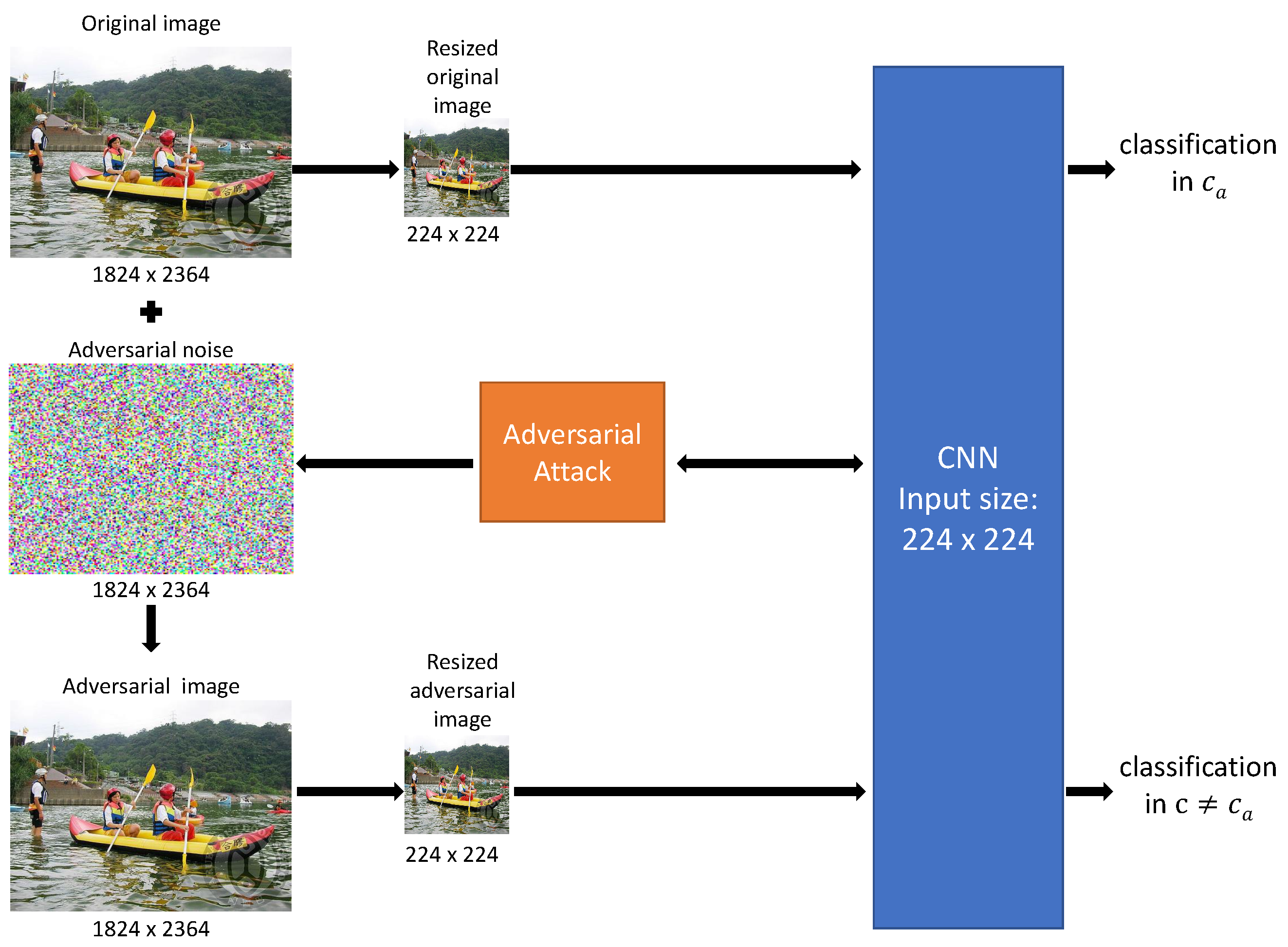
3. The Noise Blowing-Up Strategy

The method presented here (and introduced in [31]) attempts to circumvent the speed, adversity, and visual quality challenges mentioned in the Introduction, which are encountered when one intends to create HR adversarial images. While speed and adversity were successfully addressed in [29,30] via a strategy similar to some extent to the present one, the visual quality challenge remained partly unsolved. The refinement provided by our noise blowing-up strategy, which lifts to the $\mathcal{H}$ domain for any attack working in the $\mathcal{R}$ domain, addresses this visual quality issue without harming the speed and adversity features. It furthermore simplifies and generalises the attack scheme described in [29,30].

In a nutshell, the noise blowing-up strategy applied to an attack atk on a CNN $\mathcal{C}$ following a given scenario, essentially proceeds as follows.

One considers a clean image ${\mathcal{A}}_a\in \mathcal{R}$, degraded from a clean image ${\mathcal{A}}_a^{\mathrm{hr}}\in \mathcal{H}$ thanks to a degrading function $\rho$. Then one performs an attack $at{k}_{\mathcal{R},\mathcal{C}}^{scenario}$ on ${\mathcal{A}}_a$ in the $\mathcal{R}$ domain, that leads to an image $\in \mathcal{R}$, adversarial against the CNN for the considered scenario. Although getting such adversarial images in the $\mathcal{R}$ domain is crucial for obvious reasons, our strategy does not depend on how they are obtained and applies to all possible attacks $at{k}_{\mathcal{R},\mathcal{C}}^{scenario}$ working efficiently in the $\mathcal{R}$ domain. This feature contributes substantially to the flexibility of our method.

Then one computes the adversarial noise in $\mathcal{R}$ as the difference between the adversarial image and the clean image in $\mathcal{R}$. Thanks to a convenient enlarging function $\lambda$, one blows up this adversarial noise from $\mathcal{R}$ to $\mathcal{H}$. Then, one adds this blown-up noise to ${\mathcal{A}}_a^{\mathrm{hr}}$, creating that way a high-resolution image, called here the HR tentative adversarial image.

One checks whether this HR tentative adversarial image fulfills the criteria stated in the last paragraph of Section 2.3, namely becomes adversarial once degraded by the function $\rho$. Should this occur, it means that blowing up the adversarial noise in $\mathcal{R}$ has led to a noise in $\mathcal{H}$ that turns out to be also adversarial. If the blown-up noise is not sufficiently adversarial, one raises the expectations at the $\mathcal{R}$ level accordingly.

The concrete design of the noise blowing-up strategy, which aims at creating an efficient attack in the $\mathcal{H}$ domain once given an efficient attack in the $\mathcal{R}$ domain for some scenario, is given step-by-step in Section 3.1. A series of indicators is given in Section 3.2. The assessment of these indicators depends on the choice of the degrading and enlarging functions used to go from $\mathcal{H}$ to $\mathcal{R}$, and vice versa. These choices are specified in Section 4.

3.1. Constructing Images Adversarial in $\mathcal{H}$ out of Those Adversarial in $\mathcal{R}$

Given a CNN $\mathcal{C}$, the starting point is a large-size clean image ${\mathcal{A}}_a^{\mathrm{hr}}\in \mathcal{H}$.

In Step 1, one constructs its degraded image ${\mathcal{A}}_a=\rho \left({\mathcal{A}}_a^{\mathrm{hr}}\right)\in \mathcal{R}$.

In Step 2, one runs $\mathcal{C}$ on ${\mathcal{A}}_a$ to get its classification in a category $c_a$. More precisely, one gets $\mathcal{C}\left({\mathcal{A}}_a\right)=(c_a,{\tau }_a)$.

In Step 3, with notations consistent with those used in Section 2.3, one assumes given an attack $at{k}_{\mathcal{R},\mathcal{C}}^{scenario}$ on ${\mathcal{A}}_a$ in the $\mathcal{R}$ domain, that leads to an image

$${\tilde{\mathcal{D}}}_{scenario}^{\mathcal{C}}\left({\mathcal{A}}_a\right)\in \mathcal{R},$$

(6)

adversarial against CNN for the considered scenario. As already stated, how such an adversarial image is obtained does not matter. For reasons linked to Step 5 and to Step 8, one denotes $(c_{bef},{\tilde{\tau }}_{c_{bef}})$ the outcome of the classification by $\mathcal{C}$ of this adversarial image in $\mathcal{R}$. The index “$bef$” indicates that these assessments and measures take place before the noise blowing-up process per se (Steps 4, 5, 6 essentially).

Step 4 consists in getting the adversarial noise ${\mathcal{N}}^{\mathcal{C}}\left({\mathcal{A}}_a\right)\in \mathcal{R}$ as the difference

$${\mathcal{N}}^{\mathcal{C}}\left({\mathcal{A}}_a\right)={\tilde{\mathcal{D}}}_{scenario}^{\mathcal{C}}\left({\mathcal{A}}_a\right)-{\mathcal{A}}_a\in \mathcal{R}$$

(7)

of images living in $\mathcal{R}$, one being the adversarial image of the clean other.

To perform Step 5, one needs a fixed enlarging function

$$\lambda : \mathcal{R}⟶\mathcal{H}$$

(8)

that transforms any image of $\mathcal{R}$ into an image in $\mathcal{H}$. Anticipating on Step 8, it is worthwhile noting that, although the reduction function $\rho$ and the enlarging function $\lambda$ have opposite purposes, these functions are not necessarily inverse one from the other. In other words, $\rho \circ \lambda$ and $\lambda \circ \rho$ may differ from the identity maps $i{d}_{\mathcal{R}}$ and $i{d}_{\mathcal{H}}$ respectively (usually they do).

One applies the enlarging function $\lambda$ to the low-resolution adversarial noise ${\mathcal{N}}^{\mathcal{C}}\left({\mathcal{A}}_a\right)$, what leads to the blown-up noise

$${\mathcal{N}}^{hr,\mathcal{C}}\left({\mathcal{A}}_a^{\mathrm{hr}}\right)=\lambda \left({\mathcal{N}}^{\mathcal{C}}\left({\mathcal{A}}_a\right)\right)\in \mathcal{H}.$$

(9)

In Step 6, one creates the HR tentative adversarial image by adding this blown-up noise to the original high-resolution image as follows:

$${\mathcal{D}}_{scenario}^{\mathrm{hr},\mathcal{C}}\left({\mathcal{A}}_a^{\mathrm{hr}}\right)={\mathcal{A}}_a^{\mathrm{hr}}+{\mathcal{N}}^{hr,\mathcal{C}}\left({\mathcal{A}}_a^{\mathrm{hr}}\right)\in \mathcal{H}.$$

(10)

In Step 7, the application of the reduction function $\rho$ on this HD tentative adversarial image creates an image ${\mathcal{D}}_{scenario}^{\mathcal{C}}\left({\mathcal{A}}_a^{\mathrm{hr}}\right)=\rho \left({\mathcal{D}}_{scenario}^{\mathrm{hr},\mathcal{C}}\left({\mathcal{A}}_a^{\mathrm{hr}}\right)\right)$ in the $\mathcal{R}$ domain.

Finally, in Step 8, one runs $\mathcal{C}$ on ${\mathcal{D}}_{scenario}^{\mathcal{C}}\left({\mathcal{A}}_a^{\mathrm{hr}}\right)$ to get its classification $(c_{aft},{\tau }_{c_{aft}})$. The index “$aft$” indicates that these assessments and measures take place after the noise blowing-up process per se (Steps 4, 5, 6 essentially).

The attack succeeds if the conditions stated at the end of Section 2.3 are satisfied according to the considered scenario.

Remarks.—(1) For reasons explained in Step 5, there is no reason that ${\tilde{\tau }}_{c_{bef}}={\tau }_{c_{aft}}$ even when $\mathcal{C}$ classifies both images ${\tilde{\mathcal{D}}}_{scenario}^{\mathcal{C}}\left({\mathcal{A}}_a\right)$ and ${\mathcal{D}}_{scenario}^{\mathcal{C}}\left({\mathcal{A}}_a^{\mathrm{hr}}\right)$ in the same category $c=c_{bef}=c_{aft}$ (this condition is expected in the target scenario, provided this common category satisfies $c\ne c_a$). These label values are very likely to differ. This has two consequences: the first is to make mandatory the verification process performed in Step 8, let alone to make sure that the adversarial image is conveniently classified by $\mathcal{C}$ according to the considered scenario; the second is that, for the target scenario, one should set the value of ${\tilde{\tau }}_{c_{bef}}$ in a way such to ensure that the image ${\mathcal{D}}_t^{\mathrm{hr},\mathcal{C}}\left({\mathcal{A}}_a^{\mathrm{hr}}\right)$ is indeed adversarial (see Section 3.2). (2) In the context of the untarget scenario, one should make sure that $c_{aft}\ne c_a$. In the context of the target scenario, one should also aim at getting $c_{aft}=c_{bef}$ (provided one succeeds in creating an adversarial image for which $c_{bef}\ne c_a$). These requirements are likely to influence the value set to ${\tilde{\tau }}_{c_{bef}}$ as well (see Section 3.2).

Scheme (11) summarizes these steps. It shows how to create, from a target attack $at{k}_{\mathcal{R},\mathcal{C}}^{scenario}$ efficient against $\mathcal{C}$ in the $\mathcal{R}$ domain, the attack $at{k}_{\mathcal{H},\mathcal{C}}^{scenario}$ in the $\mathcal{H}$ domain obtained by the noise blowing-up strategy:

(11)

3.2. Indicators

Although both ${\tilde{\mathcal{D}}}_{scenario}^{\mathcal{C}}\left({\mathcal{A}}_a\right)$ and ${\mathcal{D}}_{scenario}^{\mathcal{C}}\left({\mathcal{A}}_a^{\mathrm{hr}}\right)$ stem from ${\mathcal{A}}_a^{\mathrm{hr}}$, belong to the same set $\mathcal{R}$ of low-resolution images, these images nevertheless differ in general, since $\rho \circ \lambda \ne i{d}_{\mathcal{R}}$. Therefore, as already stated, this fact implies that the verification process performed in Step 8 is mandatory.

For the target scenario, one aims at $c_{aft}=c_{bef}=c_t$. Since ${\tilde{\tau }}_{c_t}$ and ${\tau }_{c_t}$ are likely to differ, One measures the difference with the real-valued loss function$\mathcal{L}$ defined for ${\mathcal{A}}_a^{\mathrm{hr}}\in \mathcal{H}$ as

$${\mathcal{L}}_{\mathcal{C}}\left({\mathcal{A}}_a^{\mathrm{hr}}\right)={\tilde{\tau }}_{c_t}-{\tau }_{c_t}.$$

(12)

In particular, for the target scenario, our attack is effective if one can set accurately the value of ${\tilde{\tau }}_t$ to match the inequality ${\tau }_t\ge \tau$ for the threshold value $\tau$, or to make sure that ${\mathcal{D}}_t^{\mathcal{C}}\left({\mathcal{A}}_a^{\mathrm{hr}}\right)$ is a good enough adversarial image in the $\mathcal{R}$ domain while controlling the distance variations between ${\mathcal{A}}_a^{\mathrm{hr}}$ and the adversarial ${\mathcal{D}}_t^{\mathrm{hr},\mathcal{C}}\left({\mathcal{A}}_a^{\mathrm{hr}}\right)$.

For the untarget scenario, one aims at $c_{aft}\ne c_a$. To hope to achieve $c_{aft}\ne c_a$, one requires $c_{bef}\ne c_a$. However, this requirement alone may not be sufficient to obtain $c_{aft}\ne c_a$. Indeed, depending on the attack, the adversarial image ${\mathcal{D}}_{untarget}^{\mathcal{C}}\left({\mathcal{A}}_a^{\mathrm{hr}}\right)$ (in the $\mathcal{R}$ domain) may be very sensitive to the level of trust that ${\tilde{\mathcal{D}}}_{untarget}^{\mathcal{C}}\left({\mathcal{A}}_a^{\mathrm{hr}}\right)$ (also in the $\mathcal{R}$ domain) belongs to the category $c_{bef}$. In other words, even if the attack performed in step 3 of the noise blowing-up strategy succeeded, steps 5 to 9 may not succeed under some circumstances, and it may occur that the image resulting from these steps is classified back to $c_a$.

Although less pregnant for the target scenario, a similar sensitivity phenomenon may nevertheless occur, leading to $c_{aft}\ne c_{bef}$ (hence to $c_{aft}\ne c_t$, since $c_{bef}=c_t$ in this scenario), and therefore to an unsuccess of the noise blowing-up strategy.

For these reasons, it may be safer to ensure a “margin of security” measured as follows. One defines the Delta function ${\Delta }_{\mathcal{C}}$ for ${\mathcal{A}}_a^{\mathrm{hr}}\in \mathcal{H}$ as:

$${\Delta }_{\mathcal{C}}\left({\mathcal{A}}_a^{\mathrm{hr}}\right)={\tilde{\tau }}_{c_{bef}}-{\tilde{\tau }}_{c_{next,bef}},$$

(13)

where $c_{next,bef}$ is the second best category, namely the category c for which the label value ${\tilde{\tau }}_c$ is the highest after the label value ${\tilde{\tau }}_{c_{bef}}$ of $c_{bef}$. Enlarging the distance of the label values between the best and second best category before launching the next steps of the noise blowing-up strategy may lead to higher success rates of the strategy (see Section 6).

Remark.—Note that the present approach, at the difference of the approach, initially introduced in [29,30], does not require frequent resizing up and down via $\lambda ,\rho$ the adversarial images. In particular, if one knows how the loss function behaves (in the worst case, or in average) for a given targeted attack, then one can adjust a priori the value of $\widetilde{{\tau }_c}$ accordingly, and be satisfied with one such resizing up and down. Mutatis mutandis for the untarget attack and the Delta function.

To assess the visual variations and the noise between the images (see Section 2.1), we shall compute the $L_0^{norm},L_1^{norm},L_2^{norm}$, $L_{\infty }$, and FID values for the following pairs of images:

• ${\mathcal{A}}_a$ and ${\tilde{\mathcal{D}}}_{scenario}^{\mathcal{C}}\left({\mathcal{A}}_a^{\mathrm{hr}}\right)$ in the $\mathcal{R}$ domain. One writes $L_{p,\mathcal{R}}^{norm,adv}$ ($p=0,1,2$) and $L_{\infty ,\mathcal{R}}^{adv}$ the corresponding values.
• ${\mathcal{A}}_a^{\mathrm{hr}}$ and ${\mathcal{D}}_{scenario}^{\mathrm{hr},\mathcal{C}}\left({\mathcal{A}}_a^{\mathrm{hr}}\right)$ in the $\mathcal{H}$ domain. One writes $L_{p,\mathcal{H}}^{norm,adv}$ ($p=0,1,2$) and $L_{\infty ,\mathcal{H}}^{adv}$ the corresponding values.
• ${\mathcal{A}}_a^{\mathrm{hr}}$ and $\lambda \circ \rho \left({\mathcal{A}}_a^{\mathrm{hr}}\right)$ in the $\mathcal{H}$ domain. One writes $L_{p,\mathcal{H}}^{norm,clean}$ ($p=0,1,2$) and $L_{\infty ,\mathcal{H}}^{clean}$ the corresponding values.
• ${\mathcal{A}}_a^{\mathrm{hr}}$, $\lambda \circ \rho \left({\mathcal{A}}_a^{\mathrm{hr}}\right)$ in the $\mathcal{H}$ domain. One writes ${\mathrm{FID}}_{\mathcal{H}}^{clean}$ the corresponding values.
• ${\mathcal{A}}_a^{\mathrm{hr}}$ and ${\mathcal{D}}_{scenario}^{\mathrm{hr},\mathcal{C}}\left({\mathcal{A}}_a^{\mathrm{hr}}\right)$ in the $\mathcal{H}$ domain. One writes ${\mathrm{FID}}_{\mathcal{H}}^{adv}$ the corresponding values.

In particular, when adversarial images are involved, the comparison of some of these values between what occurs in the $\mathcal{R}$ domain, and what occurs in the $\mathcal{H}$ domain gives an insight into the weight of the noise at each level, and of the noise propagation once blown-up. Additionally, we shall as well assess the ratio:

$$\frac{L_{1,\mathcal{H}}^{norm,adv}}{L_{1,\mathcal{H}}^{norm,clean}}=\frac{L_1^{norm}({\mathcal{A}}_a^{\mathrm{hr}},{\mathcal{D}}_{scenario}^{\mathrm{hr},\mathcal{C}}\left({\mathcal{A}}_a^{\mathrm{hr}}\right))}{L_1^{norm}({\mathcal{A}}_a^{\mathrm{hr}},\lambda \circ \rho \left({\mathcal{A}}_a^{\mathrm{hr}}\right))}.$$

This ratio normalizes the weight of the noise with respect to the effect of the anyhow occurring composition $\lambda \circ \rho$. Said otherwise, it evaluates the impact created by the noise normalized by the impact created anyhow by the resizing functions.

4. Ingredients of the Experimental Study

This section specifies the key ingredients used in the experimental study performed in Section 5: degrading and enlarging functions, CNNs, HR clean images, attacks and scenarios. We also take advantage of the outcomes of [29,30,31] for the choice of some parameters used in the experimental study.

4.1. The Selection of $\rho$ and of $\lambda$

The assessment of the indicators of Section 3.2, and therefore the performances and adequacy of the resized tentative adversarial images obtained between $\mathcal{R}$ and $\mathcal{H}$, clearly depend on the reducing and enlarging functions $\rho$ and $\lambda$ selected in Scheme (11).

The combination call $(\rho ,\lambda ,\rho )$ (performed in Step 1 for the first call of $\rho$, in Step 5 for the unique call of $\lambda$, and in Step 7 for the second call of $\rho$) to the degrading and enlarging functions are “aside” of the actual attacks performed in the $\mathcal{R}$ domain. However, both the adversity and the visual quality of the HR adversarial images are highly sensitive to the selected combination.

Moreover, as pointed out in [29], enlarging functions usually have difficulties with high-frequency features. This phenomenon leads to an increased blurriness in the resulting image. Therefore, the visual quality of (and the speed to construct, see [29]) the high-resolution adversarial images obtained by our noise blowing-up strategy benefits from a scarce usage of the enlarging function. Consequently, the scheme minimizes the number of times $\lambda$ (and consequently $\rho$) are used.

We considered four non-adaptive methods that convert an image from one scale to another. Indeed, the Nearest Neighbor [44], the Bilinear method [45], the Bicubic method [46] and the Lanczos method [47,48] are among the most common interpolation algorithms, and are available in python libraries. Note that the Nearest Neighbor method is the default degradation function on Keras $load\_img$ function [35]. Tests performed in [29,30] lead to reducing the resizing functions to the Lanczsos and the Nearest methods.

We performed a case study with the 8 possible different combinations $(\rho ,\lambda ,\rho )$ obtained with the Lanczsos and the Nearest methods (see Appendix B for the full details). Its outcomes lead us to recommend the combination $(\rho ,\lambda ,\rho )=Lanczos,Lanczos,Lanczos)$ (see also Section 4.3).

4.2. The CNNs

The experimental study is performed on 10 diverse and commonly used CNNs trained on ImageNet (see [27] for the reasons for these choices). These CNNs are specified in Table 1.

Table 1. The 10 CNNs trained on ImageNet, their number of parameters (in millions), and their Top-1 and Top-5 accuracy.

${\mathcal{C}}_{\mathit{k}}$	Name of the CNN	Parameters	Top-1 Accuracy	Top-5 Accuracy
${\mathcal{C}}_1$	DenseNet121	8M	0.750	0.923
${\mathcal{C}}_2$	DenseNet169	14M	0.762	0.932
${\mathcal{C}}_3$	DenseNet201	20M	0.773	0.936
${\mathcal{C}}_4$	MobileNet	4M	0.704	0.895
${\mathcal{C}}_5$	NASNetMobile	4M	0.744	0.919
${\mathcal{C}}_6$	ResNet50	26M	0.749	0.921
${\mathcal{C}}_7$	ResNet101	45M	0.764	0.928
${\mathcal{C}}_8$	ResNet152	60M	0.766	0.931
${\mathcal{C}}_9$	VGG16	138M	0.713	0.901
${\mathcal{C}}_{10}$	VGG19	144M	0.713	0.900

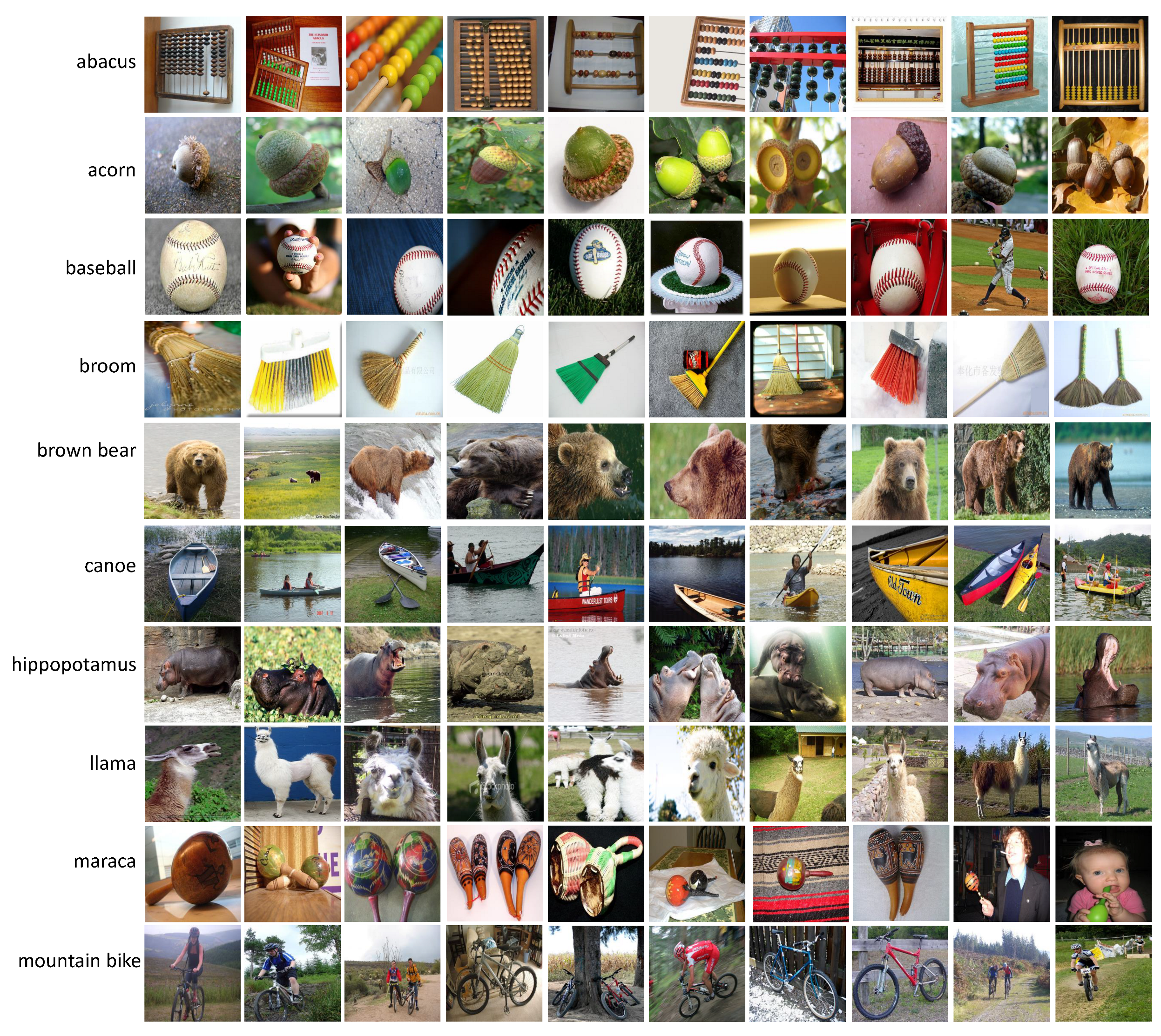
4.3. The HR Clean Images

The experiments are performed on 100 HR clean images. More specifically, Table 2 gives the 10 ancestor categories $c_a$, and the 10 corresponding target categories $c_t$ used in the $(c_a,c_t)$-target scenario whenever applicable (see Section 4.4). These categories (ancestor or target) are the same as those of [27,49], which were picked at random among the 1000 categories of ImageNet.

Table 2. For $1\le p\le 10$, the second column lists the ancestor category $c_{a_p}$ and its ordinal $1\le a_p\le 1000$ among the categories of ImageNet. Mutatis mutandis in the third column with the target category $c_{t_p}$ and ordinal $t_p$.

p	$({\mathit{c}}_{{\mathit{a}}_{\mathit{p}}},{\mathit{a}}_{\mathit{p}})$	$({\mathit{c}}_{{\mathit{t}}_{\mathit{p}}},{\mathit{t}}_{\mathit{p}})$
1	(abacus, 398)	(bannister, 421)
2	(acorn, 988)	(rhinoceros beetle, 306)
3	(baseball, 429)	(ladle, 618)
4	(broom, 462)	(dingo, 273)
5	(brown bear, 294)	(pirate, 724)
6	(canoe, 472)	(saluki, 176)
7	(hippopotamus, 344)	(trifle, 927)
8	(llama, 355)	(agama, 42)
9	(maraca, 641)	(conch, 112)
10	(mountain bike, 671)	(strainer, 828)

For each ancestor category, we picked at random 10 clean ancestor images from the ImageNet validation scheme in the corresponding $c_a$ category, provided that their size $h\times w$ satisfies $h\ge 224$ and $w\ge 224$. This requirement ensures that these images ${\mathcal{A}}_a^{\mathrm{hr}}$ belong to the $\mathcal{H}$ domain. These images are pictured in Figure A1 in Appendix A, while Table A1 gives their original sizes. Note that, out of the 100 HR clean images in Figure A1, 92 coincide with those used in [27,49] (which were picked at random in this article). We replaced the 8 remaining images used in [27,49] whose sizes did not fulfill the requirement. As a consequence, the images ${\mathcal{A}}_1^1$ and ${\mathcal{A}}_1^{10}$ in the category $c_{a_1}$, ${\mathcal{A}}_3^3$ in the category $c_{a_3}$, ${\mathcal{A}}_5^1,{\mathcal{A}}_5^2,{\mathcal{A}}_5^7$ in the category $c_{a_5}$, and ${\mathcal{A}}_9^4,{\mathcal{A}}_9^7$ in the category $c_{a_9}$ differ from those of [27,49].

Although the images ${\mathcal{A}}_q^p$ are picked from the ImageNet validation set in the categories $c_{a_q}$, CNNs may not systematically classify all of them in the “correct” category $c_{a_q}$ in the process of Steps 1 and 2 of Scheme (11). Indeed, Table A2 and Table A3 in Appendix A show that this phenomenon occurs for all CNNs, whether one uses $\rho =$ “Lanczos” (L) or “Nearest” (N). Table 3 summarizes these outcomes, where ${\mathcal{S}}_{clean}^{\mathcal{C}}\left(\rho \right)$ designates the set of “correctly” classified clean images ${\mathcal{A}}_q^p$.

Table 3. For each CNN ${\mathcal{C}}_k$ (1st row), number of clean HR images ${\mathcal{A}}_q^p$ classified by ${\mathcal{C}}_k$ in the “correct” category $c_{a_q}$ either with the degrading function $\rho =$ “Lanczos” (2nd row), or with $\rho =$ “Nearest” (3rd row).

$\mathcal{C}$	${\mathcal{C}}_1$	${\mathcal{C}}_2$	${\mathcal{C}}_3$	${\mathcal{C}}_4$	${\mathcal{C}}_5$	${\mathcal{C}}_6$	${\mathcal{C}}_7$	${\mathcal{C}}_8$	${\mathcal{C}}_9$	${\mathcal{C}}_{10}$
$\#{\mathcal{S}}_{clean}^{\mathcal{C}}\left(L\right)$	97	99	98	97	95	98	95	95	93	94
$\#{\mathcal{S}}_{clean}^{\mathcal{C}}\left(N\right)$	99	97	97	95	94	97	95	94	93	94

Table 3 shows that the sets ${\mathcal{S}}_{clean}^{\mathcal{C}}\left(L\right)$ and ${\mathcal{S}}_{clean}^{\mathcal{C}}\left(N\right)$ usually differ. Table A2 and Table A3 proves that this holds as well for $\mathcal{C}={\mathcal{C}}_7,{\mathcal{C}}_9,{\mathcal{C}}_{10}$ although both sets have the same number of elements.

In any case, the “wrongly” classified clean images are from now on disregarded since they introduce a native bias. Experiments are therefore performed only for the “correctly” classified HR clean images belonging to ${\mathcal{S}}_{clean}^{\mathcal{C}}\left(\rho \right)$.

4.4. The Attacks

We considered seven well-known attacks against the 10 CNNs given in Table 1. Table 4 lists these attacks, and specifies (with an “x”) whether we use them in the experiments for the targeted scenario, for the untargeted scenario, or for both (see Table 5 for a justification of these choices), and their white-box or black-box nature. To be more precise, if an attack admits a dual nature, namely black box and white-box (potentially semi-white-box), we consider the attack only in its more demanding black-box nature. This leads us to consider three black-box attacks (EA, AdvGAN, SimBA) and four white-box attacks (FGSM, BIM, PGD Inf, PGD L2).

Table 4. List of attacks considered, their white-box or black-box nature, and the scenarios for which they are run in the present study.

Attacks	White Box	Black Box	Targeted	Untargeted
EA		x	x	x
advGAN		x	x	x
SimBA		x		x
FGSM	x			x
BIM	x		x	x
PGD Inf	x		x	x
PGD $L2$	x		x	x

Table 5. Number of successfully generated adversarial images in the $\mathcal{R}$ domain.

Attacks	EA		AdvGAN		SimBA		FGSM		BIM		PGD Inf		PGD L2
	untarg	targ	untarg	targ	untarg	targ	untarg	targ	untarg	targ	untarg	targ	untarg	targ
${\mathcal{C}}_1$	95	89	96	81	91	0	78	0	96	68	97	96	97	82
${\mathcal{C}}_2$	95	92	94	85	94	0	63	2	98	78	99	98	99	90
${\mathcal{C}}_3$	94	90	93	82	92	0	67	1	96	71	98	98	97	85
${\mathcal{C}}_4$	94	90	81	88	91	0	64	0	96	84	97	97	97	94
${\mathcal{C}}_5$	89	77	89	74	85	0	50	0	88	56	93	83	94	71
${\mathcal{C}}_6$	95	94	92	79	90	0	84	1	96	96	97	98	96	98
${\mathcal{C}}_7$	92	87	86	78	92	0	80	1	93	93	95	95	93	93
${\mathcal{C}}_8$	86	93	88	74	78	0	75	0	94	94	95	95	89	94
${\mathcal{C}}_9$	90	92	78	58	87	0	86	3	92	76	92	93	91	83
${\mathcal{C}}_{10}$	90	94	79	59	87	1	87	1	92	77	93	94	92	84
$max$	0.546	0.555	0.762	0.481	0.508	0.041	0.993	0.457	0.999	0.999	0.999	0.999	0.999	0.999
$min$	0.007	0.550	0.003	0.031	0.038	0.041	0.050	0.257	0.258	0.289	0.524	0.721	0.277	0.221
avg	0.359	0.551	0.150	0.255	0.352	0.041	0.522	0.340	0.958	0.901	0.987	0.986	0.966	0.943

Let us now briefly describe these attacks while specifying the parameters to be used in the experiments. Note that, except (for the time being) for the EA attack, all attacks were applied with the Adversarial Robustness Toolbox (ART) [50], which is a Python library that includes several attack methods.

–EA attack [25,27] is an evolutionary algorithm-based black-box attack. It begins by creating a population of ancestor image copies and iteratively modifies their pixels over generations. The attack’s objective is defined by a fitness function that uses an individual’s $c_t$ probability obtained from the targeted CNN. The population size is set to 40, and the pixel mutation magnitude per generation is $\alpha =1/255$. The attack is executed in both targeted and untargeted scenarios. For the targeted scenario, the adversarial image’s minimum $c_t$-label value is set to $\widetilde{{\tau }_t}\ge 0.55$. The maximum number of generations is set to N = 10,000.

–Adversarial GAN attack (AdvGAN) [51] is a type of attack that operates in either a semi-whitebox or black-box setting. It uses a generative adversarial network (GAN) to create adversarial images by employing three key components: a generator, a discriminator, and the targeted neural network. During the attack, the generator is trained to produce perturbations that can convert original images into adversarial images, while the discriminator ensures that the generated adversarial image appears identical to the original image. The attack is executed in the black-box setting.

–Simple Black-box Attack (SimBA) [52] is a versatile algorithm that can be used for both black-box and white-box attacks. It works by randomly selecting a vector from a predefined orthonormal basis and adding or subtracting it from the target image. SimBA is a simple and effective method that can be used for both targeted and untargeted attacks. For our experiments, we utilized SimBA in the black-box setting with the overshoot parameter epsilon set to 0.2, batch size set to 1, and the maximum number of generations set to 10,000 for both targeted and untargeted attacks.

–Fast Gradient Sign Method (FGSM) [53] is a white-box attack that works by using the gradient of the loss function J(X,y) with respect to the input X to determine the direction in which the original input should be modified. FGSM is a one-step algorithm that can be executed quickly. In its untargeted version, the adversarial image is

$$X^{adv}=X+ϵsign\left({\Delta }_{X}J(X,c_a)\right),$$

(14)

while in its targeted version it is

$$X^{adv}=X-ϵsign\left({\Delta }_{X}J(X,c_t)\right).$$

(15)

where $ϵ$ is the perturbation size which is calculated with $L_{inf}$ norm and $\Delta$ is the gradient function. We set $eps\_step=0.01$ and $ϵ=8/255$.

–Basic Iterative Method (BIM) [54] is a white-box attack that is an iterative version of FGSM. BIM is a computationally expensive attack, as it requires calculating the gradient at each iteration. In BIM, the adversarial image $X_{adv}$ is initialized with the original image X and gradually updated over a given number of steps N as follows:

$$X_{\ell +1}^{adv}=Cli{p}_{ϵ}\{X_{\ell }^{adv}+\alpha sign\left({\Delta }_{\mathcal{A}}\left(J_{\mathcal{C}}(X_{\ell }^{adv},c_a)\right)\right)\}$$

(16)

in its untargeted version and

$$X_{\ell +1}^{adv}=Cli{p}_{ϵ}\{X_{\ell }^{adv}-\alpha sign\left({\Delta }_{\mathcal{A}}\left(J_{\mathcal{C}}(X_{\ell }^{adv},c_t)\right)\right)\},$$

(17)

in its targeted version, where $\alpha$ is the step size at each iteration and $ϵ$ is the maximum perturbation magnitude of $X^{adv}=X_N^{adv}$. We use the $eps\_step=0.1$, $max\_iter=100$, and $ϵ=2/255$.

–Projected Gradient Descent Infinite (PGD Inf) [55] is a white-box attack that is similar to the BIM attack, but with some key differences. In PGD Inf, the initial adversarial image is not set to the original image X, but rather to a random point within an $L_p$-ball around X. The distance between X and $X^{adv}$ is measured using the $L_{norm}$. For our experiments, we set the norm parameter to ∞, which indicates the use of the $L_{\infty }$ norm. We also set the step size parameter $eps\_step$ to 0.1, the batch size to 32, and the maximum perturbation magnitude $ϵ$ to 8/255.

–Projected Gradient Descent $L2$ (PGD $L2$) [55] is a white-box attack and it is similar to PGD Inf, with the difference that $L_{\infty }$ is replaced with $L_2$. We set $norm=2$, $eps\_step=0.1$, $batch\_size=32$, and $ϵ=2$.

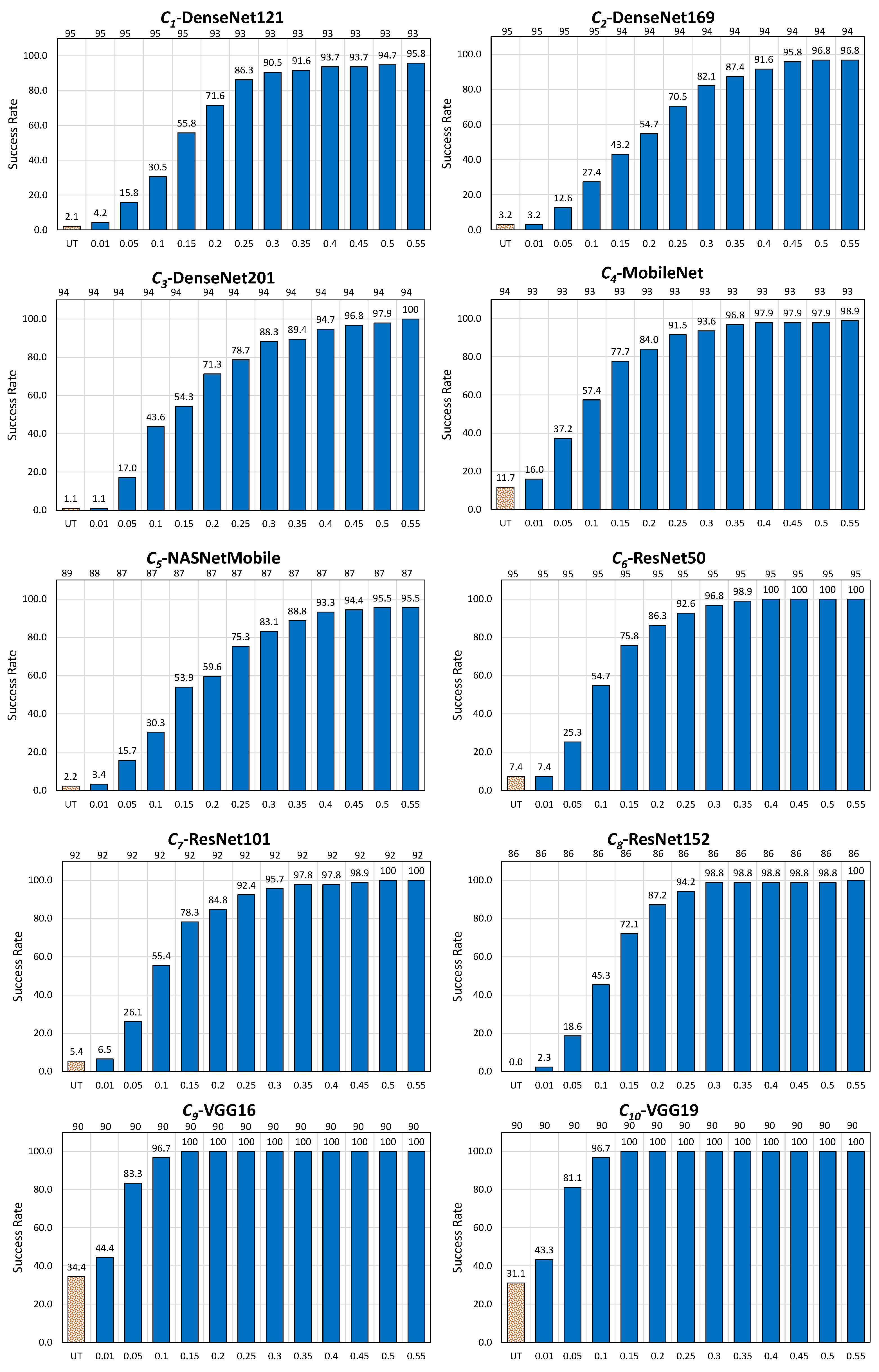
5. Experimental Results of the Noise Blowing-Up Method

The experiments, following the process implemented in Scheme (11), essentially proceed in two phases for each CNN listed in Table 1, and for each attack and each scenario specified in Table 4.

Phase 1, whose results are given in Section 5.1, mainly deals with running $at{k}_{\mathcal{R},\mathcal{C}}^{scenario}$ on degraded images in the $\mathcal{R}$ domain. It corresponds to Step 3 of Scheme (11). The results of these experiments are interpreted in Section 5.2.

Remark.—It is worthwhile noting that Step 3, which is, of course, mandatory in the whole process, should be considered an independent feature of the noise blowing-up strategy. Indeed, although its results are necessary for the experiments performed in the subsequent steps, the success or failure of Phase 1 measures the success or failure of the considered attack (EA, AdvGAN, BIM, etc.) for the considered scenario (target or untarget) in its usual environment (the low-resolution $\mathcal{R}$ domain). In other words, the outcomes of Phase 1 do not assess in any way the success or failure of the noise blowing-up strategy. This very aspect is addressed in the experiments performed in Phase 2.

Phase 2, whose results are given in Section 5.3, indeed encapsulates the essence of running $at{k}_{\mathcal{H},\mathcal{C}}^{scenario}$ via the blowing-up of the adversarial noise from $\mathcal{R}$ to $\mathcal{H}$. It corresponds to Steps 4 to 8 of Scheme (11). The results of these experiments are interpreted in Section 5.4.

5.1. Phase 1: Running $at{k}_{\mathcal{R},\mathcal{C}}^{scenario}$

Table 5 summarizes the outcome of running the attacks $at{k}_{\mathcal{R},{\mathcal{C}}_k}^{scenario}$ on the 100 clean ancestor images $\rho \left({\mathcal{A}}_q^p\right)\in \mathcal{R}$, obtained by degrading, with $\rho =$ “Lanczos” function, the HR clean images ${\mathcal{A}}_q^p$ represented in Figure A1, against the 10 CNNs ${\mathcal{C}}_1,\cdots ,C_{10}$, either for the untarget scenario, or for the $(c_a,c_t)$ target scenario.

Table 5 gives the number of successfully generated adversarial images in the $\mathcal{R}$ domain created by seven attacks against 10 CNNs, for either the targeted (targ) or the untargeted (untarg) scenario. In the last three rows, the maximum, minimum, and average dominant label values achieved by each successful targeted/untargeted attack are reported across all CNNs.

5.2. Interpretation of the Results of Phase 1

Except for SimBA and FGSM for the target scenario, one sees that all attacks are performing well for both scenarios. Given SimBA and FGSM’s poor performance in generating adversarial images for the target scenario (see Remark at the beginning of this Section), we decided to exclude them from the subsequent noise blowing-up strategy for the target scenario.

The analysis of the average dominant label values reveals as expected that white-box attacks usually create very strong adversarial images. This is the case for BIM, PGD Inf, and PGD L2 in both the targeted and untargeted scenarios. A contrario but also as expected, black-box attacks (EA, AdvGan for both scenarios, and SimBA for the untarget scenario) achieved lower label values for the target scenario and significantly lower label value of the dominant category for the untarget scenario. This specific issue (or, better said, its consequences as reported in Section 5.3 and Section 5.4) is addressed in Section 6.

5.3. Phase 2: Running $at{k}_{\mathcal{H},\mathcal{C}}^{scenario}$

For the relevant adversarial images kept from Table 5, one proceeds with the remaining steps of Scheme (11) with the extraction of the adversarial noise in the $\mathcal{R}$ domain, its blowing-up to the $\mathcal{H}$ domain, its addition to the clean HR corresponding image, and the classification by the CNN of the resulting tentative adversarial image.

The speed of the noise blowing-up method is directly impacted by the size of the clean high-resolution image (as pointed out in [31]). Therefore, representative HR clean images of large size and small sizes are required to assess the additional computational cost (both in absolute and relative terms) involved by the noise blowing-up method. To ensure a fair comparison across various attacks and CNNs, we selected for each scenario (targeted or untargeted) HR clean images where all attacks successfully generated HR adversarial images against 10 CNNs. This led to the images referred to in Table 6 (the Table indicates their respective sizes $h\times w$).

Table 6. Images employed for the assessment of the speed/overhead of the noise blowing-up method for each considered scenario and attack.

Attacks	Targeted	Untargeted
	EA, FGSM, BIM, PGD Inf, PGD L2	FGSM, BIM, PGD Inf, PGD L2
images ($h\times w$)	${\mathcal{A}}_1^{10}$ ($2448\times 3264$)	${\mathcal{A}}_6^9$ ($1536\times 2048$)
	${\mathcal{A}}_2^1$ ($374\times 500$)	${\mathcal{A}}_8^4$ ($253\times 380$)

The performance of the noise blowing-up method is summarized in Table 7 Please revise all mentions according to requested style and ensure all tables are mentioned in numerical order. for adversarial images generated by $at{k}_{\mathcal{H},\mathcal{C}}^{targeted}$, and in Table 8 for those generated by $at{k}_{\mathcal{H},\mathcal{C}}^{untargeted}$ for each CNN and attack (except $SimB{A}_{\mathcal{H},\mathcal{C}}^{targeted}$ and $FGS{M}_{\mathcal{H},\mathcal{C}}^{targeted}$ for reasons given in Section 5.2). The adversarial images in $\mathcal{R}$ used for these experiments are those referred to in Table 5.

Table 7. Performance of the Noise blowing-up strategy on adversarial images generated with attacks for the targeted scenario $(c_a,c_{bef})$ (with $c_{bef}=c_t$) against 10 CNNs. The symbol ↑ (resp. ↓) indicates the higher (resp. the lower) the value the better.

Targeted Attacks		${\mathcal{C}}_1$	${\mathcal{C}}_2$	${\mathcal{C}}_3$	${\mathcal{C}}_4$	${\mathcal{C}}_5$	${\mathcal{C}}_6$	${\mathcal{C}}_7$	${\mathcal{C}}_8$	${\mathcal{C}}_9$	${\mathcal{C}}_{10}$
EA	$\uparrow c_{aft}=c_{bef}$	81	74	80	76	61	91	86	89	92	94	824
	$c_{aft}\ne c_{bef}$	8	18	10	14	16	3	1	4	0	0
	$\downarrow c_{aft}=c_a$	8	18	10	14	3	3	1	4	0	0
	↑ SR	91.0	80.4	88.9	84.4	79.2	96.8	98.9	95.7	100	100	91.5
	$\downarrow {\mathcal{L}}_{\mathcal{C}}$	0.202	0.213	0.189	0.249	0.243	0.139	0.129	0.120	0.044	0.036	0.156
AdvGAN	$\uparrow c_{aft}=c_{bef}$	0	0	0	0	0	0	0	0	0	2	2
	$c_{aft}\ne c_{bef}$	4	4	2	5	11	8	4	3	24	21
	$\downarrow c_{aft}=c_a$	76	81	80	83	63	72	74	71	34	36
	↑ SR	0	0	0	0	0	0	0	0	0	8.7	0.9
	$\downarrow {\mathcal{L}}_{\mathcal{C}}$	0.113	0.218	0.211	0.160	0.162	0.176	0.221	0.186	0.034	0.040	0.152
BIM	$\uparrow c_{aft}=c_{bef}$	50	64	53	69	47	96	92	92	75	72	710
	$c_{aft}\ne c_{bef}$	18	14	18	15	9	0	1	2	1	5
	$\downarrow c_{aft}=c_a$	17	13	18	15	6	0	1	2	1	3
	↑ SR	73.5	83.1	74.6	82.1	83.9	100	98.9	97.9	98.6	93.5	88.6
	$\downarrow {\mathcal{L}}_{\mathcal{C}}$	0.100	0.165	0.167	0.117	0.119	0.007	0.024	0.023	0.025	0.025	0.077
PGD Inf	$\uparrow c_{aft}=c_{bef}$	96	98	97	96	78	98	95	95	93	94	940
	$c_{aft}\ne c_{bef}$	0	0	1	1	5	0	0	0	0	0
	$\downarrow c_{aft}=c_a$	0	0	1	1	4	0	0	0	0	0
	↑ SR	100	100	98.9	98.9	93.9	100	100	100	100	100	99.2
	$\downarrow {\mathcal{L}}_{\mathcal{C}}$	0.013	0.010	0.011	0.017	0.046	3$\times {10}^{-6}$	7$\times {10}^{-5}$	6$\times {10}^{-6}$	2$\times {10}^{-5}$	1$\times {10}^{-4}$	0.009
PGD L2	$\uparrow c_{aft}=c_{bef}$	69	76	75	89	64	96	92	93	82	81	817
	$c_{aft}\ne c_{bef}$	13	14	10	5	7	2	1	1	1	3
	$\downarrow c_{aft}=c_a$	13	14	10	5	4	2	1	1	1	2
	↑ SR	84.1	84.4	88.2	94.7	90.1	97.9	98.9	98.9	98.8	96.4	93.2
	$\downarrow {\mathcal{L}}_{\mathcal{C}}$	0.013	0.126	0.114	0.081	0.070	0.005	0.005	0.004	0.015	0.020	0.058
↑ Average SR		69.7	69.6	70.1	72.0	69.4	78.9	79.3	78.5	79.5	79.7	74.7
↓ Average ${\mathcal{L}}_{\mathcal{C}}$		0.114	0.146	0.138	0.125	0.128	0.065	0.076	0.067	0.024	0.024	0.091

Table 8. Performance of the Noise blowing-up technique on adversarial images generated with untargeted attacks against 10 CNNs. The symbol ↑ (resp. ↓) indicates the higher (resp. the lower) the value the better.

Untargeted Attacks		${\mathcal{C}}_1$	${\mathcal{C}}_2$	${\mathcal{C}}_3$	${\mathcal{C}}_4$	${\mathcal{C}}_5$	${\mathcal{C}}_6$	${\mathcal{C}}_7$	${\mathcal{C}}_8$	${\mathcal{C}}_9$	${\mathcal{C}}_{10}$
EA	$\uparrow c_{aft}\ne c_a$	2	3	1	11	2	7	5	0	31	28	90
	$c_{aft}=c_{bef}$	2	3	1	11	2	7	5	0	31	28
	$\downarrow c_{aft}=c_a$	93	92	93	83	87	88	87	86	59	62
	↑ SR	2.2	3.2	1.1	11.7	2.2	7.4	5.4	0.0	34.4	31.1	9.9
AdvGAN	$\uparrow c_{aft}\ne c_a$	4	8	4	4	8	7	2	6	18	22	83
	$c_{aft}=c_{bef}$	4	8	4	4	8	7	2	6	18	22
	$\downarrow c_{aft}=c_a$	92	86	89	77	81	85	84	82	60	57
	↑ SR	4.2	8.5	4.3	4.9	9.0	7.6	2.3	6.8	23.1	27.8	9.9
SimBA	$\uparrow c_{aft}\ne c_a$	25	23	22	24	18	25	32	30	31	36	266
	$c_{aft}=c_{bef}$	25	23	22	24	18	25	32	30	31	36
	$\downarrow c_{aft}=c_a$	66	71	70	67	67	65	60	48	56	51
	↑ SR	27.5	24.5	23.9	26.4	21.2	27.8	34.8	38.5	35.6	41.4	30.1
FGSM	$\uparrow c_{aft}\ne c_a$	77	60	64	63	49	84	79	75	86	87	724
	$c_{aft}=c_{bef}$	77	59	62	59	49	83	74	75	86	86
	$\downarrow c_{aft}=c_a$	1	3	3	1	1	0	1	0	0	0
	↑ SR	98.7	95.2	95.5	98.4	98.0	100.0	98.8	100.0	100.0	100.0	98.5
BIM	$\uparrow c_{aft}\ne c_a$	95	97	96	95	88	96	93	93	92	92	937
	$c_{aft}=c_{bef}$	95	96	96	92	87	96	93	93	92	92
	$\downarrow c_{aft}=c_a$	1	1	0	1	0	0	0	1	0	0
	↑ SR	99.0	99.0	100.0	99.0	100.0	100.0	100.0	98.9	100.0	100.0	99.6
PGD Inf	$\uparrow c_{aft}\ne c_a$	97	99	98	97	93	97	95	95	92	93	956
	$c_{aft}=c_{bef}$	97	99	98	97	92	97	95	95	92	93
	$\downarrow c_{aft}=c_a$	0	0	0	0	0	0	0	0	0	0
	SR	100	100	100	100	100	100	100	100	100	100	100.0
PGD L2	$\uparrow c_{aft}\ne c_a$	96	98	97	96	92	96	93	89	91	92	940
	$c_{aft}=c_{bef}$	96	98	97	96	92	96	93	89	90	92
	$\downarrow c_{aft}=c_a$	1	1	0	1	2	0	0	0	0	0
	↑ SR	99.0	99.0	100.0	99.0	97.9	100.0	100.0	100.0	100.0	100.0	99.5
↑ Average SR		61.5	61.3	60.7	62.8	61.2	63.3	63.0	63.5	70.5	71.5	63.9

For each relevant attack and CNN, the measures of a series of outcomes are given in Table 7 and Table 8.

Regarding targeted attacks (the five attacks EA, AdvGAN, BIM, PGD Inf, and PGD L2 are considered) as summarized in Table 7, the row $c_{aft}=c_{bef}$ (and $=c_t$) gives the number of adversarial images for which the noise blowing-up strategy succeeded. The row SR gives the resulting success rate in % (For example, with EA and ${\mathcal{C}}_1$, SR $=\frac{81}{89}=91\%$). The row $c_{aft}\ne c_{bef}$ reports the number of adversarial images for which the noise blowing-up strategy failed. The row $c_{aft}=c_a$ reports the number of images, among those that failed, that are classified back to $c_a$. The row ${\mathcal{L}}_{\mathcal{C}}$ gives the mean value of the loss function (see Section 3.2) for the adversarial images that succeeded, namely those referred to in the row $c_{aft}=c_{bef}$. Relevant sums or average values are given in the last column.

Regarding untargeted attacks (the seven attacks are considered) as summarized in Table 8, the row $c_{aft}\ne c_a$ gives the number of adversarial images for which the noise blowing-up strategy succeeded, and the row SR gives the resulting success rate. The row $c_{aft}=c_{bef}$ reports the number of images, among those that succeeded, that are classified in the same category as the adversarial image obtained in Phase 1. The row $c_{aft}=c_a$ reports the number of images for which the strategy failed. Relevant sums or average values are given in the last column.

To assess the visual imperceptibility of adversarial images compared to clean images, we utilize $L_p$-norms and FID values (see Section 3.2). The average (Avg) and standard deviation (StDev) values of the $L_p$-norms and FID values, across all CNNs for each attack, are provided for both targeted and untargeted scenarios in Table 9 and Table 10, respectively (see Table A6 and Table A7 for detailed report of FID values). Table 9 considers only the successful adversarial images provided in Table 7, namely those identified by $c_{aft}=c_{bef}$, provided their number is statistically relevant (what leads to the exclusion of AdvGAN images). Table 10 considers only the successful adversarial images obtained in Table 8, namely those identified by $c_{aft}\ne c_a$ (all considered attacks lead to a number of adversarial images that is statistically relevant). This is indicated by the pair “$atk/\#$ of adversarial images used”. Table 9 and Table 10 also provide an assessment of the visual impact of the resizing functions $\rho$ and $\lambda$ on the considered clean images for which adversarial images are obtained by $atk$.

Table 9. Visual quality as assessed by $L_p$-distances and FID values for the target scenario.

Targeted Attack/# of Adversarial Images Used
		EA/824		BIM/710		PGD Inf/940		PGD L2/817		Overall/3291
		Avg	StDev	Avg	StDev	Avg	StDev	Avg	StDev	Avg	StDev
$L_0$	$L_{0,\mathcal{R}}^{norm,adv}$	0.945	0.014	0.979	0.013	0.971	0.010	0.995	0.009	0.829	0.009
	$L_{0,\mathcal{H}}^{norm,adv}$	0.939	0.015	0.833	0.036	0.858	0.043	0.645	0.023	0.744	0.024
	$L_{0,\mathcal{H}}^{norm,clean}$	0.998	0.009	0.997	0.012	0.996	0.014	0.996	0.014	0.996	0.010
$L_1$	$L_{1,\mathcal{R}}^{norm,adv}$	0.047	0.078	0.009	0.035	0.010	0.003	0.003	3 $\times {10}^{-4}$	0.014	0.023
	$L_{1,\mathcal{H}}^{norm,adv}$	0.023	0.006	0.005	0.001	0.009	0.003	0.003	3 $\times {10}^{-4}$	0.009	0.002
	$L_{1,\mathcal{H}}^{norm,clean}$	0.027	0.017	0.022	0.014	0.025	0.016	0.023	0.015	0.021	0.014
	$L_{1,\mathcal{H}}^{norm,adv}$/$L_{1,\mathcal{H}}^{norm,clean}$	1.271	1.112	0.362	0.338	0.562	0.480	0.214	0.202	0.543	0.467
$L_2$	$L_{2,\mathcal{R}}^{norm,adv}$	8 $\times {10}^{-5}$	2 $\times {10}^{-5}$	2 $\times {10}^{-5}$	2 $\times {10}^{-6}$	3 $\times {10}^{-5}$	9 $\times {10}^{-6}$	1 $\times {10}^{-5}$	9 $\times {10}^{-7}$	3 $\times {10}^{-5}$	7 $\times {10}^{-6}$
	$L_{2,\mathcal{H}}^{norm,adv}$	4 $\times {10}^{-5}$	2 $\times {10}^{-5}$	8 $\times {10}^{-6}$	3 $\times {10}^{-6}$	2 $\times {10}^{-5}$	6 $\times {10}^{-6}$	7 $\times {10}^{-6}$	2 $\times {10}^{-6}$	1 $\times {10}^{-5}$	6 $\times {10}^{-6}$
	$L_{2,\mathcal{H}}^{norm,clean}$	5 $\times {10}^{-5}$	3 $\times {10}^{-5}$	5 $\times {10}^{-5}$	3 $\times {10}^{-5}$	5 $\times {10}^{-5}$	3 $\times {10}^{-5}$	5 $\times {10}^{-5}$	3 $\times {10}^{-5}$	4 $\times {10}^{-5}$	2 $\times {10}^{-5}$
$L_{\infty }$	$L_{\infty ,\mathcal{R}}^{norm,adv}$	36	11	2	0	8	0	17	4	16	4
	$L_{\infty ,\mathcal{H}}^{norm,adv}$	38	10	5	0	13	2	18	5	18	4
	$L_{\infty ,\mathcal{H}}^{norm,clean}$	129	41	125	42	127	42	125	42	119	34
FID	${\mathrm{FID}}_{\mathcal{H}}^{adv}$	17.6	6.6	5.3	2.7	13.7	9.4	7.7	4.1	11.1	5.7
	${\mathrm{FID}}_{\mathcal{H}}^{clean}$	14.4	1.2	14.2	0.7	13.9	0.3	14.2	0.5	14.2	0.7

Table 10. Visual quality as assessed by $L_p$-distances and FID values for the untargeted scenario.

Untargeted Attack/# of Adversarial Images
		EA/90		AdvGAN/83		SimBA/266		FGSM/724		BIM/937		PGD Inf/956		PGD L2/940		Overall/3996
		Avg	StDev	Avg	StDev	Avg	StDev	Avg	StDev	Avg	StDev	Avg	StDev	Avg	StDev	Avg	StDev
$L_0$	$L_{0,\mathcal{R}}^{norm,adv}$	0.822	0.150	0.838	0.088	0.994	0.050	0.990	0.017	0.980	0.013	0.974	0.011	0.993	0.010	0.942	0.048
	$L_{0,\mathcal{H}}^{norm,adv}$	0.825	0.107	0.851	0.064	0.809	0.091	0.966	0.010	0.844	0.031	0.879	0.039	0.654	0.018	0.832	0.051
	$L_{0,\mathcal{H}}^{norm,clean}$	0.996	0.015	0.998	0.011	0.995	0.016	0.998	0.006	0.996	0.014	0.996	0.014	0.996	0.014	0.997	0.013
$L_1$	$L_{1,\mathcal{R}}^{norm,adv}$	0.011	0.005	0.021	0.011	0.008	0.003	0.031	0.001	0.006	0.001	0.012	0.003	0.004	2 $\times {10}^{-4}$	0.013	0.003
	$L_{1,\mathcal{H}}^{norm,adv}$	0.010	0.005	0.019	0.009	0.007	0.003	0.026	0.001	0.005	0.001	0.011	0.003	0.003	3 $\times {10}^{-4}$	0.012	0.003
	$L_{1,\mathcal{H}}^{norm,clean}$	0.020	0.012	0.025	0.012	0.023	0.015	0.027	0.017	0.025	0.017	0.025	0.018	0.025	0.018	0.025	0.015
	$L_{1,\mathcal{H}}^{norm,adv}$/$L_{1,\mathcal{H}}^{norm,clean}$	0.808	1.055	0.761	0.055	0.606	0.931	1.461	1.284	0.343	0.327	0.680	0.608	0.205	0.197	0.695	0.637
$L_2$	$L_{2,\mathcal{R}}^{norm,adv}$	3 $\times {10}^{-5}$	2 $\times {10}^{-5}$	9 $\times {10}^{-5}$	5 $\times {10}^{-5}$	3 $\times {10}^{-5}$	9 $\times {10}^{-6}$	8 $\times {10}^{-5}$	2 $\times {10}^{-6}$	2 $\times {10}^{-5}$	1 $\times {10}^{-6}$	4 $\times {10}^{-5}$	9 $\times {10}^{-6}$	1 $\times {10}^{-5}$	3 $\times {10}^{-12}$	4 $\times {10}^{-5}$	1 $\times {10}^{-5}$
	$L_{2,\mathcal{H}}^{norm,adv}$	2 $\times {10}^{-5}$	1 $\times {10}^{-5}$	3 $\times {10}^{-5}$	2 $\times {10}^{-5}$	1 $\times {10}^{-5}$	7 $\times {10}^{-6}$	4 $\times {10}^{-5}$	1 $\times {10}^{-5}$	9 $\times {10}^{-6}$	3 $\times {10}^{-6}$	2 $\times {10}^{-5}$	7 $\times {10}^{-6}$	7 $\times {10}^{-6}$	2 $\times {10}^{-6}$	2 $\times {10}^{-5}$	8 $\times {10}^{-5}$
	$L_{2,\mathcal{H}}^{norm,clean}$	4 $\times {10}^{-5}$	2 $\times {10}^{-5}$	5 $\times {10}^{-5}$	3 $\times {10}^{-5}$	5 $\times {10}^{-5}$	3 $\times {10}^{-5}$	6 $\times {10}^{-5}$	3 $\times {10}^{-5}$	5 $\times {10}^{-5}$	3 $\times {10}^{-5}$	5 $\times {10}^{-5}$	3 $\times {10}^{-5}$	5 $\times {10}^{-5}$	3 $\times {10}^{-5}$	5 $\times {10}^{-5}$	3 $\times {10}^{-5}$
$L_{\infty }$	$L_{\infty ,\mathcal{R}}^{norm,adv}$	17	8	103	33	13	6	8	0	2	0	8	0	16	4	24	7
	$L_{\infty ,\mathcal{H}}^{norm,adv}$	16	8	103	39	13	6	20	1	5	0	14	1	17	4	27	8
	$L_{\infty ,\mathcal{H}}^{norm,clean}$	119	46	139	41	121	43	132	40	127	42	127	42	126	42	127	42
FID	${\mathrm{FID}}_{\mathcal{H}}^{adv}$	3.7	1.9	15.1	2.9	8.5	3.9	49.5	12.3	5.7	2.8	23.9	18.9	8.8	4.8	16.5	6.7
	${\mathrm{FID}}_{\mathcal{H}}^{clean}$	14.5	4.6	24.4	7.6	15.5	2.5	16.1	1.6	14.1	0.5	14.0	0.3	13.5	2.1	16.0	2.7

Under these conditions, Table 11 for the target scenario (respectively Table 12 for the untarget scenario) provides the execution times in seconds (averaged over the 10 CNNs for each attack and scenario) for each step of the noise blowing-up method, as described in Scheme (11), for the generation of HR adversarial images from large ${\mathcal{A}}_1^{10}$ and small ${\mathcal{A}}_2^1$ HR clean images (respectively large ${\mathcal{A}}_6^9$ and small ${\mathcal{A}}_8^4$ HR clean images).

Table 11. In the target scenario, for each considered attack $atk$, execution time (in seconds, averaged over the 10 CNNs) of each step of Scheme (11) for the generation of HR adversarial images for the HR clean images ${\mathcal{A}}_1^{10}$ and ${\mathcal{A}}_2^1$. The Overhead column provides the cumulative time of all steps except Step 3. The ‰ column displays the relative per mille additional time of the Overhead as compared to the time required by $atk$ performed in Step 3.

$\mathit{atk}$	Images	Step 1	Step 2	Step 3	Step 4	Step 5	Step 6	Step 7	Step 8	Overhead	‰
EA	${\mathcal{A}}_1^{10}$	0.144	0.047	848.7	3 $\times {10}^{-4}$	0.053	0.101	0.363	0.048	0.757	0.89
	${\mathcal{A}}_2^1$	0.010	0.048	443.2	3 $\times {10}^{-4}$	0.003	0.002	0.011	0.047	0.122	0.28
FGSM	${\mathcal{A}}_1^{10}$	0.148	0.050	59.2	2 $\times {10}^{-4}$	0.045	0.103	0.360	0.049	0.755	12.75
	${\mathcal{A}}_2^1$	0.009	0.049	58.1	2 $\times {10}^{-4}$	0.003	0.002	0.011	0.046	0.120	2.06
BIM	${\mathcal{A}}_1^{10}$	0.143	0.049	83.8	2 $\times {10}^{-4}$	0.045	0.103	0.356	0.049	0.744	8.88
	${\mathcal{A}}_2^1$	0.009	0.047	97.5	2 $\times {10}^{-4}$	0.003	0.002	0.010	0.046	0.118	1.22
PGD Inf	${\mathcal{A}}_1^{10}$	0.143	0.048	90.7	2 $\times {10}^{-4}$	0.045	0.102	0.357	0.049	0.744	8.21
	${\mathcal{A}}_2^1$	0.009	0.051	88.3	2 $\times {10}^{-4}$	0.003	0.002	0.010	0.046	0.122	1.38
PGD L2	${\mathcal{A}}_1^{10}$	0.141	0.048	104.2	2 $\times {10}^{-4}$	0.044	0.101	0.350	0.047	0.732	7.02
	${\mathcal{A}}_2^1$	0.009	0.048	106.3	2 $\times {10}^{-4}$	0.003	0.002	0.010	0.046	0.118	1.11
AVG	${\mathcal{A}}_1^{10}$	0.144	0.048		2 $\times {10}^{-4}$	0.047	0.102	0.357	0.048	0.746
	${\mathcal{A}}_2^1$	0.009	0.049		2 $\times {10}^{-4}$	0.003	0.002	0.010	0.046	0.120

Table 12. In the untargeted scenario, for each considered attack $atk$, execution time (in seconds, averaged over the 10 CNNs) of each step of Scheme (11) for the generation of HR adversarial images for the HR clean images ${\mathcal{A}}_6^9$ and ${\mathcal{A}}_8^4$. The Overhead column provides the cumulative time of all steps except Step 3. The ‰ column displays the relative per mille additional time of the Overhead as compared to the time required by $atk$ performed in Step 3.

	Images	Step 1	Step 2	Step 3	Step 4	Step 5	Step 6	Step 7	Step 8	Overhead	‰
FGSM	${\mathcal{A}}_6^9$	0.056	0.042	66.3	2 $\times {10}^{-4}$	0.021	0.037	0.136	0.042	0.334	5.04
	${\mathcal{A}}_8^4$	0.007	0.045	67.2	2 $\times {10}^{-4}$	0.002	0.001	0.005	0.042	0.103	1.53
BIM	${\mathcal{A}}_6^9$	0.055	0.042	78.9	2 $\times {10}^{-4}$	0.021	0.038	0.135	0.042	0.333	4.22
	${\mathcal{A}}_8^4$	0.007	0.043	79.1	2 $\times {10}^{-4}$	0.002	0.001	0.005	0.042	0.101	1.27
PGD Inf	${\mathcal{A}}_6^9$	0.056	0.043	80.9	2 $\times {10}^{-4}$	0.020	0.038	0.137	0.042	0.336	4.15
	${\mathcal{A}}_8^4$	0.007	0.043	81.8	2 $\times {10}^{-4}$	0.002	0.001	0.005	0.042	0.100	1.23
PGD L2	${\mathcal{A}}_6^9$	0.055	0.043	80.9	2 $\times {10}^{-4}$	0.021	0.038	0.137	0.042	0.337	4.17
	${\mathcal{A}}_8^4$	0.007	0.045	81.5	2 $\times {10}^{-4}$	0.002	0.001	0.005	0.040	0.101	1.24
AVG	${\mathcal{A}}_6^9$	0.055	0.043		2 $\times {10}^{-4}$	0.021	0.038	0.136	0.042	0.335
	${\mathcal{A}}_8^4$	0.007	0.044		2 $\times {10}^{-4}$	0.002	0.001	0.005	0.041	0.101

The Overhead column provides the time of the noise blowing-up method per se, namely computed as the cumulative time of all steps of Scheme (11) except Step 3. The ‰ column displays the relative per mille additional time of the overhead of the noise blowing-up method as compared to the underlying attack $atk$ performed in Step 3.

5.4. Interpretation of the Results of Phase 2

In the targeted scenario, the noise blowing-up strategy achieved an overall average success rate (overall attacks and CNNs) of $74.7\%$ (see Table 7).

Notably, the strategy performed close to perfection with PGD Inf, achieving an average success rate of $99.2\%$ (and minimal loss of $0.009$). The strategy performed also very well with PGD L2, EA, and BIM, with average success rates of $93.2\%$, $91.5\%$, and $88.6\%$, respectively. In contrast, the strategy performed poorly with AdvGAN, achieving a success rate oscillating between $0\%$ (for 8 CNNs) and $8.7\%$, leading to an average success rate of $0.9\%$.

The reason for the success of the noise blowing-up strategy for PGD Inf, PGD L2, EA and BIM, and its failure for AdvGAN is essentially due to the behavior, for these attacks, of the average label values of the dominant categories obtained in Table 5, hence is due to a phenomenon occurring before the noise blowing-up process per se.

Indeed, these values are very high for the white-box attacks PGD Inf ($0.986$), PGD L2 ($0.943$), and BIM ($0.901$), and are quite high for EA ($0.551$). However, this value is very low for AdvGAN ($0.255$).

The adversarial noises, obtained after Phase 1 (in the $\mathcal{R}$ domain) by all attacks except AdvGAN, are particularly robust, and “survive” the Phase 2 treatment: The noise blowing-up process did not significantly reduce their adversarial properties legacy, and the derived adversarial images, obtained after the noise blowing-up process, remained in the target category.

The situation differs for AdvGAN: After Phase 1, the target category is only modestly dominating other categories, and one (or more) other categories achieve only slightly weaker label values than the dominating target category. Consequently, the adversarial noise becomes highly susceptible to even minor perturbations, with the effect that these perturbations can easily cause transitions between categories.

In the untargeted scenario, the noise blowing-up strategy achieved an overall average success rate (overall attacks and CNNs) of $63.9\%$ (see Table 8).

The strategy performed perfectly or close to perfection with all white-box attacks, namely PGD Inf (average success rate of $100\%$), BIM ($99.6\%$), PGD L2 ($99.5\%$) and FGSM ($98.5\%$). A contrario, the strategy performed weakly or even poorly for all black-box attacks, namely SimBA ($30.1\%$), AdvGAN ($9.9\%$), and EA ($9.9\%$).

The reason for these differences in the successes of the strategy according to the considered attacks is the same as seen before in the target scenario: the behavior of the average label values of the dominating category obtained in Table 5 (hence, in this case too, before the noise blowing-up process).

Indeed, these values are very high or fairly high for PGD Inf ($0.987$), BIM ($0.958$), PGD L2 ($0.966$), and FGSM ($0.522$). However, they are much lower for EA ($0.359$), SimBA ($0.352$), and AdvGAN ($0.150$).

The adversarial noises, obtained after Phase 1 by all white-box attacks, are particularly robust, and those obtained by all black-box attacks are less resilient. In this latter case, the adversarial noise leveraged to create the tentative adversarial image by the noise blowing-up process is much more sensitive to minor perturbations, with similar consequences as those already encountered in the target scenario.

Visual quality of the adversarial images: The values of $L_{0,\mathcal{R}}^{norm,adv}$ in Table 9 (resp. Table 10) show that the attacks performed for the target scenario manipulate on average $82\%$ of the pixels of the downsized (hence in $\mathcal{R}$) clean image (resp. $94\%$ for the untarget scenario).

Nevertheless, the values of $L_{0,\mathcal{H}}^{norm,adv}$ in both tables (hence in the larger $\mathcal{H}$ domain, after the noise blowing-up process) are lower, with an overall average of $74\%$ for the targeted scenario (resp. $83\%$ for the untargeted scenario). This trend is consistent across all $L_p$ values ($p=0,1,2,\infty$), with $L_{p,\mathcal{R}}^{norm,adv}$ generally higher than the corresponding $L_{p,\mathcal{H}}^{norm,adv}$ values for all attacks (the values are closely aligned, though, for $p=\infty$).

Additionally, ${\mathrm{FID}}_{\mathcal{H}}^{adv}$ values, comparing clean and adversarial images obtained by the noise blowing-up method, ranging between $5.3$ (achieved by BIM) and $17.6$ in the targeted scenario (with average $11.1$, see Table 9), and between $3.7$ (achieved by EA) and $49.5$ in the untargeted scenario (with average $16.5$, see Table 10), are significantly low (it is not uncommon to have values in the range 300–500). In other words, the adversarial images maintain a visual quality and proximity to their clean counterparts.

It is important to highlight that the simple operation of scaling down and up the clean images results in even larger $L_{p,\mathcal{H}}^{norm,clean}$ values than $L_{p,\mathcal{H}}^{norm,adv}$ for $p=0,1,\infty$ for all attacks and scenarios (see Table 9 and Table 10; note that the values for $p=2$ are too small to assess the phenomenon described above). When one compares ${\mathrm{FID}}_{\mathcal{H}}^{clean}$ to ${\mathrm{FID}}_{\mathcal{H}}^{adv}$, the same phenomenon occurs for three out of 4 targeted attacks (EA is the exception), and for five out of 7 untargeted attacks (FGSM and PGD Inf being the exceptions).

Said otherwise, the interpolation techniques usually cause more visual damage than the attacks themselves, at least as measured by these indicators.

Figure 3 provides images representative of this general behavior. Evidence is furthermore supported numerically by the $L_{p,\mathcal{H}}^{norm,clean}$, $L_{p,\mathcal{H}}^{norm,adv}$ ($p=0,1,\infty$) and the ${\mathrm{FID}}_{\mathcal{H}}^{clean}$, ${\mathrm{FID}}_{\mathcal{H}}^{adv}$ values deduced from these images.

Figure 3. Examples of images for which the interpolation techniques cause more visual damage than the attacks themselves. Clean HR images ${\mathcal{A}}_a^{\mathrm{hr}}$ in the 1st column; corresponding non-adversarial HR resized images $\lambda \circ \rho \left({\mathcal{A}}_a^{\mathrm{hr}}\right)$ in the 2nd column, with values of $L_{p,\mathcal{H}}^{norm,clean}$, $p=0,1,\infty$ and ${\mathrm{FID}}_{\mathcal{H}}^{clean}$ underneath (in that order); adversarial HR images in the 3rd column ($atk=$ EA, $\mathcal{C}={\mathcal{C}}_4$, target scenario) and in the 4th column ($atk=$ BIM, $\mathcal{C}={\mathcal{C}}_6$, untarget scenario), with $L_{p,\mathcal{H}}^{norm,adv}$, $p=0,1,\infty$, and ${\mathrm{FID}}_{\mathcal{H}}^{adv}$ underneath (in that order). To enhance visibility, consider zooming in for a clearer view.

More precisely, the 1st column of Figure 3 displays the HR clean images ${\mathcal{A}}_1^2$, ${\mathcal{A}}_6^3$, and ${\mathcal{A}}_{10}^{10}$. The 2nd column displays the non-adversarial $\lambda \circ \rho \left({\mathcal{A}}_a^{\mathrm{hr}}\right)\in \mathcal{H}$ images, as well as the corresponding $L_{p,\mathcal{H}}^{norm,clean}$$(p=0,1,\infty )$ and ${\mathrm{FID}}_{\mathcal{H}}^{clean}$ values (in that order).

HR adversarial images ${\mathcal{D}}_{tar}^{\mathrm{hr},\mathcal{C}}\left({\mathcal{A}}_a^{\mathrm{hr}}\right)$ are displayed in the 3rd and 4th columns: For $atk=$ EA performed on ${\mathcal{C}}_4=$ MobileNet for the targeted scenario in the 3rd column, and for $atk=$ BIM on ${\mathcal{C}}_6=$ ResNet50 for the untargeted scenario in the 4th column. The corresponding numerical values of $L_{p,\mathcal{H}}^{norm,adv}$ ($p=0,1,\infty$) and of ${\mathrm{FID}}_{\mathcal{H}}^{adv}$ (in that order) are provided as well.

Speed of the noise blowing-up method: The outcomes of Table 11 and Table 12 for the overhead of the noise blowing-up method (all steps except Step 3) and its relative cost as compared to the actual attack (performed in Step 3) are twofold.

Firstly, the performance of the noise blowing-up strategy depends on the size of the image: It is substantially faster (between $3.24$ times and $6.31$ times on average) for smaller than for larger HR clean images.

Secondly, and this is probably the most important outcome of both, the noise blowing-up method demonstrates exceptional speed both in absolute and in relative terms, and consequently an exceptionally minimal overhead, even for large-size HR clean images.

Indeed, the overhead ranges between $0.100$ s and $0.757$ s on average over 10 CNNs ($0.100$ s achieved in the untargeted scenario for $atk=$ PGD Inf and ${\mathcal{A}}_8^4$; $0.757$ seconds achieved in the targeted scenario for $atk=$ EA and ${\mathcal{A}}_1^{10}$). This is to compare to the extreme timing values of the attacks performed in Step 3, ranging between $58.1$ and $848.7$ s all in all (and ranging between $81.8$ and $848.7$ s for the cases related to the $0.100$ and $0.757$ s referred to).

Looking at the relative weight of the overhead as compared to $atk$ is even more saying: It ranges between $0.28$‰and $12.75$‰, hence is almost negligible.

6. Revisiting the Failed Cases with ${\Delta }_{\mathcal{C}}$

The summary of Section 5.4 is essentially threefold. Firstly, the noise blowing-up strategy performs very well and with a negligible timing overhead in the target scenario for all five relevant attacks except AdvGAN, and in the untargeted scenario for all four white-box attacks but not for the three black-box attacks. Secondly, the poor performances of the strategy for AdvGAN (target scenario and untargeted scenario), EA (untargeted scenario), and SimBA (untargeted scenario) are essentially due to too low requirements put on these attacks during Phase 1 (Step 3 of Scheme (11), hence ahead of the noise blowing-up process). Thirdly, although between $74\%$ and $83\%$ of the pixels are modified on average, the adversarial images remain visually very close to their corresponding clean images, and actually and surprisingly the attacks themselves tend to reduce the differences introduced by the interpolation functions.

We revisit these failed cases and make use of the Delta function ${\Delta }_{\mathcal{C}}$ introduced in Section 3.2 for this purpose. Indeed, we identified the origin of the encountered issues as essentially due to the too low distance between the label values of the dominating category and its closest competitors, hence due to a very small value of ${\Delta }_{\mathcal{C}}$ for the considered images and CNNs.

Given ${\mathcal{A}}_a^{\mathrm{hr}}$ and ${\mathcal{A}}_a$ (Step 1), and $c_a$ (Step 2), we study in this Subsection how setting the increase of the values of ${\Delta }_{\mathcal{C}}$ as a requirement in Step 3 of Scheme (11) impacts the success rate of the noise blowing-up strategy for the failed cases. Note that putting additional requirements on ${\Delta }_{\mathcal{C}}$ may lead to lesser adversarial images at the end of Phase 1 as ${\Delta }_{\mathcal{C}}$ increases.

We limit this study to $atk=$ EA (untargeted scenario) and $atk=$ AdvGAN (untargeted and target scenario). We regrettably exclude SimBA since we do not have access to its code.

6.1. Revisiting the Failed Cases in Both Scenarios

The untargeted scenario revisited for $\mathit{atk}=$ EA and $\mathit{atk}=$ AdvGAN. The new consideration of the failed cases proceeds by taking a hybrid approach in Step 3, leading to two successive sub-steps Step 3(a) and Step 3(b).

Step 3(a) consists in running $at{k}_{\mathcal{R},\mathcal{C}}^{untarget}$ until it succeeds in creating a first adversarial image in $\mathcal{R}$ classified outside the ancestor category $c_a$. The obtained category $c_{bef}\ne c_a$ is therefore the most promising category outside $c_a$.

In Step 3(b), we change the version of the attack and run $at{k}_{\mathcal{R},\mathcal{C}}^{target}$ on the adversarial image obtained at the end of Step 3(a) for the target scenario $(c_a,c_{bef})$, with a (more demanding) stop condition defined by a threshold value on ${\Delta }_{\mathcal{C}}$ set at will.

Remarks: (1) To summarize this hybrid approach, Step 3(a) identifies the most promising category $c_{bef}$ outside $c_a$ (and does so by “pushing down” the $c_a$ label value until another category $c_{bef}$ shows up), and Step 3(b) “pushes further” the attack in the direction of $c_{bef}$ until the label value of this dominant category is sufficiently ahead of all other competitors. (2) Although this hybrid approach mixes the untargeted and the target versions of the attack (be it EA or AdvGAN), it fits the untargeted attack scenario nevertheless. Indeed, the category $c_{bef}\ne c_a$ is not chosen a priori as would be the case in the target scenario but is obtained alongside the attack, and is an outcome of $at{k}_{\mathcal{R},\mathcal{C}}^{untarget}$.

The target scenario revisited for $\mathit{atk}=$ AdvGAN. We address the failed cases by requiring in Step 3 of Scheme (11), that ${\tilde{\mathcal{D}}}_{target}^{\mathcal{C}}\left({\mathcal{A}}_a\right)\in \mathcal{R}$ is classified in $c_t$ and that ${\Delta }_{\mathcal{C}}\left({\mathcal{A}}_a^{\mathrm{hr}}\right)$ is large enough.

6.2. Outcome of Revisiting the Failed Cases

One constructs the graph of the evolution of the success rate ($y-axis$, in %) of the noise blowing-up strategy performed for the considered attack for the untargeted scenario according to step-wise increasing values (x-axis) set to ${\Delta }_{\mathcal{C}}$.

Figure 4 for $atk=$ EA (untargeted scenario), Figure 5 for $atk=$ AdvGAN (untargeted scenario) and Figure 6 for $atk=$ AdvGAN (targeted scenario) picture this evolution for an example, namely ${\mathcal{C}}_4$—MobileNet (a), on average over the 10 CNNs (b), and per CNN for all considered images (c).

Figure 4. Performance of the noise blowing-up method for EA in the untargeted scenario with the increased strength of adversarial images: (a) specifically for ${\mathcal{C}}_4$, (b) averaged across 10 CNNs, and (c) overall report for all CNNs. In (a,b), ${\Delta }_{\mathcal{C}}$ values are displayed at the bottom, and the resulting number of used images is at the top.

Figure 5. Performance of the noise blowing-up method for AdvGAN in the untargeted scenario with the increased strength of adversarial images: (a) specifically for ${\mathcal{C}}_4$, (b) averaged across 10 CNNs, and (c) overall report for all CNNs. In (a,b), ${\Delta }_{\mathcal{C}}$ values are displayed at the bottom, and the resulting number of used images is at the top.

Figure 6. Performance of the noise blowing-up method for AdvGAN in the target scenario with the increased strength of adversarial images: (a) specifically for ${\mathcal{C}}_4$, (b) averaged across 10 CNNs, and (c) overall report for all CNNs. In (a,b), ${\Delta }_{\mathcal{C}}$ values are displayed at the bottom, and the resulting number of used images is at the top.

UT (resp. T) in (a) and (b) of Figure 4 and Figure 5 (resp. of Figure 6) recalls the “original” success rate achieved by the noise blowing-up method in creating adversarial images without putting extra conditions on ${\Delta }_{\mathcal{C}}$ (see Table 8, resp. Table 7). The values at the top of the Figures are the number of images obtained after Phase 1, as ${\Delta }_{\mathcal{C}}$ increases.

Detailed reports for each CNN can be found in the Appendix C, Figure A2, Figure A3 and Figure A4.

In the untargeted scenario for $atk=$ EA, the approach adopted for the revisited failed cases turns out to be overwhelmingly successful, and this in a uniform way over the 10 CNNs. The overall number of considered images drops only by $0.6\%$, namely from 920 to 914 (in the example of ${\mathcal{C}}_4$, this drop is of one image only), while the success rate drastically increases from an original $9.9\%$ to $98.7\%$. In the example of ${\mathcal{C}}_4$, the success rate increases from $11.7\%$ to $98.9\%$; a success rate of $100\%$ is even achieved for six out of 10 CNNs, even for moderate values of ${\Delta }_{\mathcal{C}}$.

In the untargeted scenario for $atk=$ AdvGAN, the approach is also successful, but to a lesser extent, and with variations among the CNNs. The overall number of considered images drops by $43\%$, namely from 876 to 500 images (in the example of ${\mathcal{C}}_4$, this drop amounts to 22 images, hence almost $27\%$ less images), while the success rate increases from an original $9.9\%$ to $73.1\%$ (in the example of ${\mathcal{C}}_4$, the success rate increases from $4.9\%$ to $71.2\%$). Apart from ${\mathcal{C}}_2$ and ${\mathcal{C}}_5$, where the success rate of the revisited method achieves at most $50\%$ and $25.8\%$, all CNNs are reasonably well deceived by the method; the success rate achieves even $100\%$ for two of them, and this for moderate values of ${\Delta }_{\mathcal{C}}$.

In the targeted scenario, for $atk=$ AdvGAN, the approach also proves useful, but to a lesser extent as above, and with larger variations among the CNNs. The overall number of considered images drops by $21\%$, namely from 758 to 594 images (from 88 to 72 images, hence almost $18\%$ less images for ${\mathcal{C}}_4$), while the success rate increases from an original $0.3\%$ to $50.8\%$ (in the example of ${\mathcal{C}}_4$, the success rate increases from $0\%$ to $34.7\%$). It is worthwhile noting that the method works to perfection with a success rate reaching $100\%$ for two CNNs (${\mathcal{C}}_9$ and ${\mathcal{C}}_{10}$), even with a moderate ${\Delta }_{\mathcal{C}}$ value.

Table 13 summarizes the outcomes of the numerical experiments when ${\Delta }_{\mathcal{C}}$ is set to the demanding value $0.55$. As a consequence, it is advisable to set (for Phase 1, Step 3) ${\tilde{\tau }}_{c_{bef}}$ to $0.78$ for $E{A}_{untarg}$, to $0.76$ for $AdvGA{N}_{targ}$, and to $0.79$ for $AdvGA{N}_{untarg}$ to be on the safe side (these values exceed the maxima referred to in Table 13).

Table 13. Minimum, maximum, and mean of the label values ${\tilde{\tau }}_{c_{bef}}$ of adversarial images in the $\mathcal{R}$ domain (Phase 1, Step 3) when ${\Delta }_{\mathcal{C}}$ is set to 0.55 per CNN.

	${\mathit{EA}}_{\mathit{untarg}}$			${\mathit{AdvGAN}}_{\mathit{targ}}$			${\mathit{AdvGAN}}_{\mathit{untarg}}$
	Min	Max	Mean	Min	Max	Mean	Min	Max	Mean
${\mathcal{C}}_1$	0.587	0.779	0.723	0.575	0.731	0.636	0.588	0.770	0.690
${\mathcal{C}}_2$	0.593	0.778	0.725	0.583	0.689	0.633	0.619	0.766	0.710
${\mathcal{C}}_3$	0.597	0.777	0.720	0.613	0.757	0.662	0.594	0.772	0.701
${\mathcal{C}}_4$	0.572	0.771	0.657	0.571	0.688	0.624	0.581	0.771	0.654
${\mathcal{C}}_5$	0.564	0.775	0.653	0.572	0.739	0.633	0.582	0.748	0.646
${\mathcal{C}}_6$	0.610	0.780	0.725	0.587	0.741	0.655	0.581	0.778	0.691
${\mathcal{C}}_7$	0.587	0.778	0.725	0.604	0.749	0.655	0.610	0.767	0.691
${\mathcal{C}}_8$	0.603	0.777	0.724	0.586	0.756	0.654	0.606	0.788	0.699
${\mathcal{C}}_9$	0.593	0.778	0.709	0.584	0.733	0.633	0.594	0.775	0.674
${\mathcal{C}}_{10}$	0.593	0.779	0.708	0.584	0.749	0.632	0.605	0.775	0.677
Avg	0.590	0.777	0.707	0.586	0.733	0.641	0.596	0.771	0.683

Finally, experiments show that the visual quality of the HR adversarial images obtained by the revised method remains outstanding. We illustrate this statement in Figure 7 on an example, where ${\Delta }_{\mathcal{C}}$ is set to $0.55$ (the highest and most demanding value considered in the present study), and the CNN is ${\mathcal{C}}_4$. In Figure 7, (a) represents the HR clean image ${\mathcal{A}}_2^3$ classified by ${\mathcal{C}}_4$ as belonging to the “acorn” category with corresponding label value $0.90$, (b) the adversarial image created by the strategy applied to the EA attack in the untargeted scenario (classified as “snail” with label value $0.61$), (c) the adversarial image created by the strategy with AdvGAN in the untargeted scenario (classified as “dung beetle” with label value $0.55$), and (d) the adversarial image created by the strategy with AdvGAN in the targeted scenario (classified as “rhinoceros beetle” with label value $0.43$). The images speak for themselves as far as visual quality is concerned.

Figure 7. Sample of HR adversarial images generated by the noise blowing-up strategy for the EA and AdvGAN attacks in the untargeted scenario, and the AdvGAN attack in the targeted scenario against ${\mathcal{C}}_4=$ MobileNet, with ${\Delta }_{\mathcal{C}}$ set to 0.55 in the $\mathcal{R}$ domain. Classification (dominant category and label value) of ${\mathcal{C}}_4$ are displayed at the bottom. (a) Clean image acorn: 0.90. (b) ${\mathrm{EA}}_{untarg}$ snail: 0.61. (c) ${\mathrm{AdvGAN}}_{untarg}$ dung_beetle: 0.55. (d) ${\mathrm{AdvGAN}}_{targ}$ rhinoceros_beetle: 0.43.

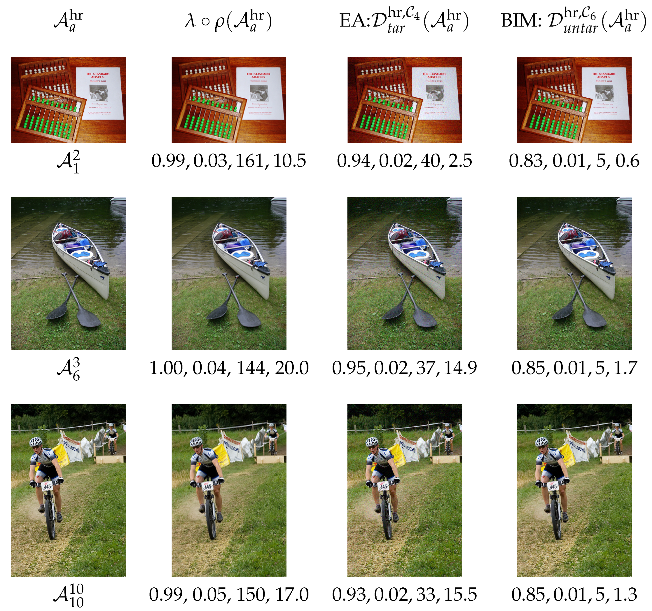
7. Comparison of the Lifting Method and of the Noise Blowing-Up Method

This section provides a comparison between the outcomes of our adversarial noise blowing-up strategy and those of the lifting method introduced in [29,30].

We shall see on three highly challenging examples, that the noise blowing-up strategy leads to a substantial visual quality gain as compared with the lifting method of [29,30] (both strategies achieve comparable and negligible timing overheads as compared to the actual underlying attacks performed). Indeed, the visual quality gain is particularly flagrant when one zooms on some areas that remained visually problematic with the method used in [29,30].

7.1. The Three HR Images, the CNN, the Attack, the Scenario

We make here a case study with three HR images (two of which have been considered in [31]), with $\mathcal{C}=$ VGG-16 trained on ImageNet, for the EA-based black-box targeted attack given in Section 4.4.

The three HR pictures are represented in Table 14. They are the comics Spiderman picture (${\mathcal{A}}_1^{\mathrm{hr}}$ retrieved from the Internet and under Creative Commons License), an artistic picture graciously provided by the French artist Speedy Graphito (${\mathcal{A}}_2^{\mathrm{hr}}$ pictured in [56]) and Hippopotamus image (${\mathcal{A}}_3^{\mathrm{hr}}={\mathcal{A}}_7^2$) taken from Figure A1. An advantage of adding artistic images is that, while a human may have difficulties in classifying them in any category, CNNs do it.

Table 14. Three clean HR images ${\mathcal{A}}_a^{\mathrm{hr}}$, their original size, the classification of VGG-16 as $(c_a,{\tau }_a)$ of their reduced versions $\rho \left({\mathcal{A}}_a^{\mathrm{hr}}\right)$ (with $\rho =$ “Lanczos”), and the target category.

a	1	2	3
${\mathcal{A}}_a^{\mathrm{hr}}$
$h\times w$	$800\times 1280$	$1710\times 1740$	$1200\times 1600$
$(c_a,{\tau }_a)$	(Comic Book, 0.4916)	(Coffee Mug, 0.0844)	(Hippopotamus, 0.9993)
$c_t$	altar	hamper	trifle

7.2. Implementation and Outcomes

Regarding implementation issues, we use $(\rho ,\lambda )=$ (Lanczos, Lanczos) for both the lifting method of [29,30] and the noise blowing-up method presented here, whenever needed.

In terms of the steps described in Section 3.1, note that both strategies coincide up to Step 3 included, and start to differ from Step 4 on. In particular, the attack process (Step 3) in the $\mathcal{R}$ domain is the same for both strategies. In the present case, one shall apply the EA-based targeted attack in the $\mathcal{R}$ domain, with the aim to create a $0.55$-strong adversarial image. In other words, ${\tilde{\tau }}_{bef}\ge 0.55$ (with notations consistent with Section 3). This process succeeded for the three examples.

Figure 8, Figure 9 and Figure 10 provide a visual comparison (both globally and on some zoomed area) of a series of images in the $\mathcal{H}$ domain for $a=1,2,3$, respectively: (a) the clean image ${\mathcal{A}}_a^{\mathrm{hr}}$, (b) the non-adversarial resized image $\lambda \circ \rho \left({\mathcal{A}}_a^{\mathrm{hr}}\right)$, (c) the adversarial image in $\mathcal{H}$ obtained by the lifting method of [29,30], (d) the adversarial image in $\mathcal{H}$ obtained by the noise blowing-up method. The non-adversarial image referred to in (b) remains classified by $\mathcal{C}$ in the $c_a$ category, and the adversarial images referred to in (c) and (d) are classified in the $c_t$ category mentioned in Table 14, with $c_t$-label values indicated in the Figures.

Figure 8. Visual comparison in the $\mathcal{H}$ domain of (a) the clean image ${\mathcal{A}}_1^{\mathrm{hr}}$, (b) its non-adversarial resized version, the adversarial image obtained with ${\mathrm{EA}}^{\mathrm{target},\mathcal{C}}$ for $\mathcal{C}=$ VGG-16, (c) by the lifting method of [29,30], and (d) by the noise blowing-up method. Both non-adversarial images are classified as “comic books”, (a) with label value $0.49$ and (b) with label value $0.45$. Both HR adversarial images are classified as “altar”, (c) with label value $0.52$, and (d) with label value $0.41$.

Figure 9. Visual comparison in the $\mathcal{H}$ domain of (a) the clean image ${\mathcal{A}}_2^{\mathrm{hr}}$, (b) its non-adversarial resized version, the adversarial image obtained with ${\mathrm{EA}}^{\mathrm{target},\mathcal{C}}$ for $\mathcal{C}=$ VGG-16, (c) by the lifting method of [29,30], and (d) by the noise blowing-up method. Both non-adversarial images are classified as “Coffee Mug”, (a) with label value $0.08$ and (b) with label value $0.08$. Both HR adversarial images are classified as “Hamper”, (c) with label value $0.51$, and (d) with label value $0.53$.

Figure 10. Visual comparison in the $\mathcal{H}$ domain of (a) the clean image ${\mathcal{A}}_3^{\mathrm{hr}}$, (b) its non-adversarial resized version, the adversarial image obtained with ${\mathrm{EA}}^{\mathrm{target},\mathcal{C}}$ for $\mathcal{C}=$ VGG-16, (c) by the lifting method of [29,30], and (d) by the noise blowing-up method. Both non-adversarial images are classified as “hippopotamus”, (a) with label value $0.99$ and (b) with label value $0.99$. Both HR adversarial images are classified as “trifle”, (c) with label value $0.51$, and (d) with label value $0.50$.

With notations consistent with Table 9 and Table 10, and with the exponent $adv,lift$, and $adv,noise$ indicating respectively that the adversarial images are obtained via the lifting method, and by the noise blowing-up method respectively, Table 15 gives a numerical assessment of the visual quality of the different HR images (b), (c), (d) compared to the clean ones (a) of Figure 8, Figure 9 and Figure 10, as measured by $L_p$ distances and FID values.

Table 15. Numerical assessment of the visual quality of the different HR images (b), (c), (d) compared to the clean ones (a) of Figure 8, Figure 9 and Figure 10, as measured by $L_p$ distances and FID values.

		${\mathcal{A}}_1^{\mathbf{hr}}$	${\mathcal{A}}_2^{\mathbf{hr}}$	${\mathcal{A}}_3^{\mathbf{hr}}$
$L_0$	$L_{0,\mathcal{H}}^{norm,clean}$	0.963	0.938	0.999
	$L_{0,\mathcal{H}}^{norm,adv,lift}$	0.973	0.970	0.969
	$L_{0,\mathcal{H}}^{norm,adv,noise}$	0.920	0.960	0.961
$L_1$	$L_{1,\mathcal{H}}^{norm,clean}$	0.071	0.037	0.029
	$L_{1,\mathcal{H}}^{norm,adv,lift}$	0.075	0.049	0.049
	$L_{1,\mathcal{H}}^{norm,adv,noise}$	0.021	0.028	0.032
$L_2$	$L_{2,\mathcal{H}}^{norm,clean}$	6 $\times {10}^{-5}$	2 $\times {10}^{-5}$	2 $\times {10}^{-5}$
	$L_{2,\mathcal{H}}^{norm,adv,lift}$	6 $\times {10}^{-5}$	2 $\times {10}^{-5}$	3 $\times {10}^{-5}$
	$L_{2,\mathcal{H}}^{norm,adv,noise}$	2 $\times {10}^{-5}$	1 $\times {10}^{-5}$	2 $\times {10}^{-5}$
$L_{\infty }$	$L_{\infty ,\mathcal{H}}^{norm,clean}$	244	174	191
	$L_{\infty ,\mathcal{H}}^{norm,adv,lift}$	245	163	198
	$L_{\infty ,\mathcal{H}}^{norm,adv,noise}$	27	30	58
FID	${\mathrm{FID}}_{\mathcal{H}}^{clean}$	180.5	45.5	50.4
	${\mathrm{FID}}_{\mathcal{H}}^{adv,lift}$	221.9	44.1	64.1
	${\mathrm{FID}}_{\mathcal{H}}^{adv,noise}$	55.3	34.9	21.9

Figure 8, Figure 9 and Figure 10 show that, at some distance, both the non-adversarial resized image (b) and the HR adversarial images (c) and (d) seem to have a good visual quality as compared to the HR clean image (a). However, the zoomed areas show that details from the HR clean images become blurry in the HR adversarial images obtained by the lifting method (c) and in the non-adversarial resized images (b). Moreover, a human eye is not able to distinguish the blurriness that occurs in (b) from the one that shows up in (c): The loss of visual quality looks the same in both cases. However, a loss of visual quality does not occur (at least to the same extent) in the HR adversarial images obtained by the noise blowing-up method (d). These observations are also sustained numerically by Table 15: $L_{p,\mathcal{H}}^{norm,clean}$ and $L_{p,\mathcal{H}}^{norm,adv,lift}$, as well as ${\mathrm{FID}}_{\mathcal{H}}^{clean}$ and ${\mathrm{FID}}_{\mathcal{H}}^{adv,lift}$ are close one to the other, while $L_{p,\mathcal{H}}^{norm,adv,noise}$ and ${\mathrm{FID}}_{\mathcal{H}}^{adv,noise}$ achieve much smaller values than their above counterparts. In particular, we see and measure in these examples, that the noise blowing-up method largely compensates for the negative visual impact of the resizing interpolation functions.

In other words, the adversarial images displayed by the noise blowing-up method in (d) are visually very close to the original clean images (a), while the adversarial images displayed by the lifting method in (c) are visually very close to the non-adversarial resized images in (b).

These experiments strongly speak in favor of our noise blowing-up method, despite the fact that interpolation scaling-up methods $\lambda$ result in a loss of high-frequency features in the $\mathcal{H}$ domain (as seen in (b) and (c)). More precisely, our noise blowing-up method essentially avoids (and even corrects, as shows the behavior of by $L_p$ and FID values) this later issue, while the lifting method does not.

8. Conclusions

In this extensive study, we exposed in detail the noise blowing-up strategy to create high-quality high-resolution images adversarial against convolutional neural networks, and indistinguishable from the original clean images.

This strategy is designed to apply to any attack (black-box or white-box), to any scenario (targeted or untargeted scenario), to any CNN, and to any clean image.

We performed an extensive experimental study on 10 state-of-the-art and diverse CNNs, with 100 high-resolution clean images, three black-box (EA, AdvGAN, SimBA), and four white-box (FGSM, BIM, PGD Inf, PGD L2) attacks, applied in the target and the untarget scenario whenever possible.

This led to the construction of $4110$ adversarial images for the target scenario and $3996$ adversarial images for the untarget scenario. Therefore, the noise blowing-up method achieved an overall average success rate of $74.7\%$ in the target scenario, and of $63.9\%$ in the untarget scenario; the strategy performing perfectly or close to perfection (with a success rate of $100\%$ or close to it) for many attacks.

We then focused on the failed cases. We showed that a minor additional requirement in one step of the strategy led to a substantial success rate increase (e.g., from circa $9.9\%$ to $98.7\%$ in the untarget scenario for the EA attack).

All along, we showed that the additional time required to perform our noise blowing-up strategy is negligible as compared to the actual cost of the underlying attack on which the strategy applies.

Finally, we compared our noise blowing-up method to another generic method, namely the lifting method. We showed that the visual quality and indistinguishability of the adversarial images obtained by our noise blowing-up strategy substantially outperform those of the adversarial images obtained by the lifting method. We also showed that applying our noise blowing-up strategy substantially corrects some visual blurriness artifacts caused natively by interpolation resizing functions.

Clearly, the noise blowing-up strategy, which essentially amounts to the addition to the clean high-resolution image of one layer of “substantial” adversarial noise, blown-up from $\mathcal{R}$ to $\mathcal{H}$, is subject to a series of refinements and variants. For instance, one may instead consider adding to the clean image several “thin” layers of “moderate” blown-up adversarial noise. This would present at least two advantages. Firstly, one can parallelize this process. Secondly, depending on how adding different layers of adversarial noise impacts the overall ${\tau }_{c_{aft}}$-value, one could consider relaxing the expectations on the ${\tilde{\tau }}_{c_{bef}}$ value for each run of the attack in the $\mathcal{R}$ domain, and still meet ${\tau }_{c_{aft}}$ and ${\Delta }_{\mathcal{C}}$ preset thresholds by adding up wisely the successive layers of noise. Both advantages may lead to a substantial speed-up of the process, and potentially to an increased visual quality. One could also consider applying the strategy to the flat scenario, where all ℓ label values are almost equidistributed, henceforth the CNN considers that all categories are almost equally likely (even this variant admits variants, e.g., where one specifies a number $2\le x\le \ell$ of dominating categories for which the attack would create an appropriate flatness).

Another promising direction comes from the observation that in the present method as well as in the method introduced in [29,30], the considered attacks explore a priori the whole image space. In future work, we intend to explore the possibility of restricting the size of the zones to explore. Provided the kept zones are meaningful (in a sense to be defined), one could that way design an additional generic method which, combined with the one presented in this paper, could lead, at a lower computational cost, to high-resolution adversarial images of very good quality, especially if one pays attention to high-frequency areas.

References

- Taye, M.M. Theoretical Understanding of Convolutional Neural Network: Concepts, Architectures, Applications, Future Directions. Computation 2023, 11, 52. [Google Scholar] [CrossRef]
- Sun, Y.; Xue, B.; Zhang, M.; Yen, G.G. Evolving deep convolutional neural networks for image classification. IEEE Trans. Evol. Comput. 2019, 24, 394–407. [Google Scholar] [CrossRef]
- Szegedy, C.; Zaremba, W.; Sutskever, I.; Bruna, J.; Erhan, D.; Goodfellow, I.J.; Fergus, R. Intriguing properties of neural networks. In Proceedings of the 2nd International Conference on Learning Representations, ICLR 2014, Banff, AB, Canada, 14–16 April 2014. [Google Scholar]
- Gao, H.; Cheng, B.; Wang, J.; Li, K.; Zhao, J.; Li, D. Object classification using CNN-based fusion of vision and LIDAR in autonomous vehicle environment. IEEE Trans. Ind. Inform. 2018, 14, 4224–4231. [Google Scholar] [CrossRef]
- Coşkun, M.; Uçar, A.; Yildirim, Ö.; Demir, Y. Face recognition based on convolutional neural network. In Proceedings of the 2017 International Conference on Modern Electrical and Energy Systems (MEES), Kremenchuk, Ukraine, 15–17 November 2017; pp. 376–379. [Google Scholar]
- Yang, S.; Wang, W.; Liu, C.; Deng, W. Scene understanding in deep learning-based end-to-end controllers for autonomous vehicles. IEEE Trans. Syst. Man Cybern. Syst. 2018, 49, 53–63. [Google Scholar] [CrossRef]
- Ghosh, A.; Jana, N.D.; Das, S.; Mallipeddi, R. Two-Phase Evolutionary Convolutional Neural Network Architecture Search for Medical Image Classification. IEEE Access 2023, 11, 115280–115305. [Google Scholar] [CrossRef]
- Abdou, M.A. Literature review: Efficient deep neural networks techniques for medical image analysis. Neural Comput. Appl. 2022, 34, 5791–5812. [Google Scholar] [CrossRef]
- Chugh, A.; Sharma, V.K.; Kumar, S.; Nayyar, A.; Qureshi, B.; Bhatia, M.K.; Jain, C. Spider monkey crow optimization algorithm with deep learning for sentiment classification and information retrieval. IEEE Access 2021, 9, 24249–24262. [Google Scholar] [CrossRef]
- Fahfouh, A.; Riffi, J.; Mahraz, M.A.; Yahyaouy, A.; Tairi, H. PV-DAE: A hybrid model for deceptive opinion spam based on neural network architectures. Expert Syst. Appl. 2020, 157, 113517. [Google Scholar] [CrossRef]
- Cao, J.; Lam, K.Y.; Lee, L.H.; Liu, X.; Hui, P.; Su, X. Mobile augmented reality: User interfaces, frameworks, and intelligence. ACM Comput. Surv. 2023, 55, 1–36. [Google Scholar] [CrossRef]
- Coskun, H.; Yiğit, T.; Üncü, İ.S. Integration of digital quality control for intelligent manufacturing of industrial ceramic tiles. Ceram. Int. 2022, 48, 34210–34233. [Google Scholar] [CrossRef]
- Khan, M.J.; Singh, P.P. Advanced road extraction using CNN-based U-Net model and satellite imagery. E-Prime Electr. Eng. Electron. Energy 2023, 5, 100244. [Google Scholar] [CrossRef]
- Saralioglu, E.; Gungor, O. Semantic segmentation of land cover from high resolution multispectral satellite images by spectral-spatial convolutional neural network. Geocarto Int. 2022, 37, 657–677. [Google Scholar] [CrossRef]
- Zhang, Y.; Liu, Y.; Liu, J.; Miao, J.; Argyriou, A.; Wang, L.; Xu, Z. 360-attack: Distortion-aware perturbations from perspective-views. In Proceedings of the IEEE/CVF Conference on Computer Vision and Pattern Recognition, New Orleans, LA, USA, 18–24 June 2022; pp. 15035–15044. [Google Scholar]
- Meng, W.; Xing, X.; Sheth, A.; Weinsberg, U.; Lee, W. Your online interests: Pwned! a pollution attack against targeted advertising. In Proceedings of the 2014 ACM SIGSAC Conference on Computer and Communications Security, Scottsdale, AZ, USA, 3–7 November 2014; pp. 129–140. [Google Scholar]
- Hardt, M.; Nath, S. Privacy-aware personalization for mobile advertising. In Proceedings of the 2012 ACM Conference on Computer and Communications Security, Raleigh, NC, USA, 16–18 October 2012; pp. 662–673. [Google Scholar]
- Biggio, B.; Corona, I.; Maiorca, D.; Nelson, B.; Šrndić, N.; Laskov, P.; Giacinto, G.; Roli, F. Evasion attacks against machine learning at test time. In Proceedings of the Joint European Conference on Machine Learning and Knowledge Discovery in Databases, Prague, Czech Republic, 23–27 September 2013; Springer: Berlin/Heidelberg, Germany, 2013; pp. 387–402. [Google Scholar]
- Carlini, N.; Wagner, D. Towards evaluating the robustness of neural networks. In Proceedings of the 2017 IEEE Symposium on Security and Privacy (SP), San Jose, CA, USA, 22–26 May 2017; pp. 39–57. [Google Scholar]
- Wang, Y.; Liu, J.; Chang, X.; Misic, J.V.; Misic, V.B. IWA: Integrated Gradient based White-box Attacks for Fooling Deep Neural Networks. arXiv 2021, arXiv:2102.02128. [Google Scholar] [CrossRef]
- Mohammadian, H.; Ghorbani, A.A.; Lashkari, A.H. A gradient-based approach for adversarial attack on deep learning-based network intrusion detection systems. Appl. Soft Comput. 2023, 137, 110173. [Google Scholar] [CrossRef]
- Papernot, N.; McDaniel, P.; Goodfellow, I.; Jha, S.; Celik, Z.B.; Swami, A. Practical black-box attacks against machine learning. In Proceedings of the 2017 ACM on Asia Conference on Computer and Communications Security, Abu Dhabi, United Arab Emirates, 2–7 April 2017; pp. 506–519. [Google Scholar]
- Andriushchenko, M.; Croce, F.; Flammarion, N.; Hein, M. Square attack: A query-efficient black-box adversarial attack via random search. In European Conference on Computer Vision; Springer: Cham, Switzerland, 2020; pp. 484–501. [Google Scholar]
- Chitic, R.; Bernard, N.; Leprévost, F. A proof of concept to deceive humans and machines at image classification with evolutionary algorithms. In Proceedings of the Intelligent Information and Database Systems, 12th Asian Conference, ACIIDS 2020, Phuket, Thailand, 23–26 March 2020; Springer: Berlin/Heidelberg, Germany, 2020; pp. 467–480. [Google Scholar]
- Chitic, R.; Leprévost, F.; Bernard, N. Evolutionary algorithms deceive humans and machines at image classification: An extended proof of concept on two scenarios. J. Inf. Telecommun. 2020, 5, 121–143. [Google Scholar] [CrossRef]
- Al-Ahmadi, S.; Al-Eyead, S. GAN-based Approach to Crafting Adversarial Malware Examples against a Heterogeneous Ensemble Classifier. In Proceedings of the 19th International Conference on Security and Cryptography—Volume 1: SECRYPT, INSTICC, Lisbon, Portugal, 11–13 July 2022; SciTePress: Setúbal, Portugal, 2022; pp. 451–460. [Google Scholar] [CrossRef]
- Topal, A.O.; Chitic, R.; Leprévost, F. One evolutionary algorithm deceives humans and ten convolutional neural networks trained on ImageNet at image recognition. Appl. Soft Comput. 2023, 143, 110397. [Google Scholar] [CrossRef]
- Deng, J.; Dong, W.; Socher, R.; Li, L.J.; Li, K.; Fei-Fei, L. The ImageNet Image Database. 2009. Available online: http://image-net.org (accessed on 14 April 2024).
- Leprévost, F.; Topal, A.O.; Avdusinovic, E.; Chitic, R. A Strategy Creating High-Resolution Adversarial Images against Convolutional Neural Networks and a Feasibility Study on 10 CNNs. J. Inf. Telecommun. 2022, 7, 89–119. [Google Scholar] [CrossRef]
- Leprévost, F.; Topal, A.O.; Avdusinovic, E.; Chitic, R. Strategy and Feasibility Study for the Construction of High Resolution Images Adversarial against Convolutional Neural Networks. In Proceedings of the Intelligent Information and Database Systems, 13th Asian Conference, ACIIDS 2022, Ho-Chi-Minh-City, Vietnam, 28–30 November 2022; Springer: Berlin/Heidelberg, Germany, 2022; pp. 467–480. [Google Scholar]
- Leprévost, F.; Topal, A.O.; Mancellari, E. Creating High-Resolution Adversarial Images Against Convolutional Neural Networks with the Noise Blowing-Up Method. In Intelligent Information and Database Systems; Nguyen, N.T., Boonsang, S., Fujita, H., Hnatkowska, B., Hong, T.P., Pasupa, K., Selamat, A., Eds.; Springer: Singapore, 2023; pp. 121–134. [Google Scholar]
- Van Rossum, G.; Drake, F.L. Python 3 Reference Manual; CreateSpace: Scotts Valley, CA, USA, 2009. [Google Scholar]
- Oliphant, T.E. Guide to NumPy; Trelgol, 2006; Available online: https://web.mit.edu/dvp/Public/numpybook.pdf (accessed on 14 April 2024).
- Abadi, M.; Agarwal, A.; Barham, P.; Brevdo, E.; Chen, Z.; Citro, C.; Corrado, G.S.; Davis, A.; Dean, J.; Devin, M.; et al. TensorFlow: Large-Scale Machine Learning on Heterogeneous Systems. 2015. Available online: https://www.tensorflow.org (accessed on 14 April 2024).
- Keras. 2015. Available online: https://keras.io (accessed on 14 April 2024).
- Van der Walt, S.; Schönberger, J.L.; Nunez-Iglesias, J.; Boulogne, F.; Warner, J.D.; Yager, N.; Gouillart, E.; Yu, T.; The Scikit-Image Contributors. scikit-image: Image processing in Python. PeerJ 2014, 2, e453. [Google Scholar] [CrossRef] [PubMed]
- Heusel, M.; Ramsauer, H.; Unterthiner, T.; Nessler, B.; Hochreiter, S. Gans trained by a two time-scale update rule converge to a local nash equilibrium. Adv. Neural Inf. Process. Syst. 2017, 30. [Google Scholar] [CrossRef]
- Luo, C.; Lin, Q.; Xie, W.; Wu, B.; Xie, J.; Shen, L. Frequency-driven imperceptible adversarial attack on semantic similarity. In Proceedings of the IEEE/CVF Conference on Computer Vision and Pattern Recognition, New Orleans, LA, USA, 18–24 June 2022; pp. 15315–15324. [Google Scholar]
- Chen, F.; Wang, J.; Liu, H.; Kong, W.; Zhao, Z.; Ma, L.; Liao, H.; Zhang, D. Frequency constraint-based adversarial attack on deep neural networks for medical image classification. Comput. Biol. Med. 2023, 164, 107248. [Google Scholar] [CrossRef]
- Liu, J.; Lu, B.; Xiong, M.; Zhang, T.; Xiong, H. Adversarial Attack with Raindrops. arXiv 2023, arXiv:2302.14267. [Google Scholar]
- Zhao, Z.; Liu, Z.; Larson, M. Towards large yet imperceptible adversarial image perturbations with perceptual color distance. In Proceedings of the IEEE/CVF Conference on Computer Vision and Pattern Recognition, Seattle, WA, USA, 13–19 June 2020; pp. 1039–1048. [Google Scholar]
- Johnson, J.; Alahi, A.; Fei-Fei, L. Perceptual losses for real-time style transfer and super-resolution. In Proceedings of the Computer Vision–ECCV 2016: 14th European Conference, Amsterdam, The Netherlands, 11–14 October 2016; Proceedings, Part II 14. Springer: Cham, Switzerland, 2016; pp. 694–711. [Google Scholar]
- Szegedy, C.; Vanhoucke, V.; Ioffe, S.; Shlens, J.; Wojna, Z. Rethinking the Inception Architecture for Computer Vision. arXiv 2015, arXiv:1512.00567. [Google Scholar]
- Patel, V.; Mistree, K. A review on different image interpolation techniques for image enhancement. Int. J. Emerg. Technol. Adv. Eng. 2013, 3, 129–133. [Google Scholar]
- Agrafiotis, D. Chapter 9—Video Error Concealment. In Academic Press Library in signal Processing; Theodoridis, S., Chellappa, R., Eds.; Elsevier: Amsterdam, The Netherlands, 2014; Volume 5, pp. 295–321. [Google Scholar] [CrossRef]
- Keys, R. Cubic convolution interpolation for digital image processing. IEEE Trans. Acoust. Speech Signal Process. 1981, 29, 1153–1160. [Google Scholar] [CrossRef]
- Duchon, C.E. Lanczos filtering in one and two dimensions. J. Appl. Meteorol. Climatol. 1979, 18, 1016–1022. [Google Scholar] [CrossRef]
- Parsania, P.S.; Virparia, P.V. A comparative analysis of image interpolation algorithms. Int. J. Adv. Res. Comput. Commun. Eng. 2016, 5, 29–34. [Google Scholar] [CrossRef]
- Chitic, R.; Topal, A.O.; Leprévost, F. ShuffleDetect: Detecting Adversarial Images against Convolutional Neural Networks. Appl. Sci. 2023, 13, 4068. [Google Scholar] [CrossRef]
- Nicolae, M.I.; Sinn, M.; Tran, M.N.; Buesser, B.; Rawat, A.; Wistuba, M.; Zantedeschi, V.; Baracaldo, N.; Chen, B.; Ludwig, H.; et al. Adversarial Robustness Toolbox v1.2.0. arXiv 2018, arXiv:1807.01069. [Google Scholar]
- Xiao, C.; Li, B.; Zhu, J.Y.; He, W.; Liu, M.; Song, D. Generating Adversarial Examples with Adversarial Networks. arXiv 2019, arXiv:1801.02610. [Google Scholar]
- Guo, C.; Gardner, J.; You, Y.; Wilson, A.G.; Weinberger, K. Simple black-box adversarial attacks. In Proceedings of the International Conference on Machine Learning, PMLR, Long Beach, CA, USA, 9–15 June 2019; pp. 2484–2493. [Google Scholar]
- Goodfellow, I.J.; Shlens, J.; Szegedy, C. Explaining and Harnessing Adversarial Examples. arXiv 2015, arXiv:1810.00069. [Google Scholar]
- Kurakin, A.; Goodfellow, I.J.; Bengio, S. Adversarial examples in the physical world. arXiv 2016, arXiv:1607.02533. [Google Scholar]
- Madry, A.; Makelov, A.; Schmidt, L.; Tsipras, D.; Vladu, A. Towards Deep Learning Models Resistant to Adversarial Attacks. arXiv 2019, arXiv:1706.06083. [Google Scholar]
- SpeedyGraphito. Mes 400 Coups; Panoramart: France, 2020. [Google Scholar]
Disclaimer/Publisher’s Note: The statements, opinions and data contained in all publications are solely those of the individual author(s) and contributor(s) and not of MDPI and/or the editor(s). MDPI and/or the editor(s) disclaim responsibility for any injury to people or property resulting from any ideas, methods, instructions or products referred to in the content. |
© 2024 by the authors. Licensee MDPI, Basel, Switzerland. This article is an open access article distributed under the terms and conditions of the Creative Commons Attribution (CC BY) license (https://creativecommons.org/licenses/by/4.0/).