A Deep Learning Approach to Semantic Segmentation of Steel Microstructures

Featured Application

A segmentation tool for microconstituents recognition in steel optical micrographs.

Abstract

The utilization of convolutional neural networks (CNNs) for semantic segmentation has proven to be successful in various applications, such as autonomous vehicle environment analysis, medical imaging, and satellite imagery. In this study, we investigate the application of different segmentation networks, including Deeplabv3+, U-Net, and SegNet, each recognized for their effectiveness in semantic segmentation tasks. Additionally, in the case of Deeplabv3+, we leverage the use of pre-trained ResNet50, ResNet18 and MobileNetv2 as feature extractors for a comprehensive analysis of steel microstructures. Our specific focus is on distinguishing perlite and ferrite phases in micrographs of low-carbon steel specimens subjected to annealing heat treatment. The micrographs obtained using an optical microscope are manually segmented. Preprocessing techniques are then applied to create a dataset for building a supervised learning model. In the results section, we discuss in detail the performance of the obtained models and the metrics used. The models achieve a remarkable 95% to 98% accuracy in correctly labeling pixels for each phase. This underscores the effectiveness of our approach in differentiating perlite and ferrite phases within steel microstructures.

1. Introduction

The recognition of the microconstituents of a steel micrograph is a complicated task and only within the reach of highly qualified personnel with broad experience in the field of materials science. Manual identification of steel phases can be a tedious and error-prone task; therefore, machine learning (ML) models have emerged as valuable complements to the traditional visual inspection methods employed by metallurgists. In recent years, many studies have addressed the challenge of developing artificial intelligence techniques that enable computers to handle complex tasks, such as microstructure identification [1,2,3] and the inference of properties through these identification techniques utilizing ML has been investigated [4,5,6,7], yielding promising advancements. Nevertheless, given the complexity involved in microstructure identification, particularly within steel micrographs, the adoption of advanced techniques becomes necessary. For the realization of an effective image segmentation in the context of steel microstructures, a powerful tool, such as a deep neural network, is required.

In previous work [8], it was determined that, for the categorization of steel microstructures, convolutional neural networks exhibit a notable superiority over classical machine learning algorithms. The present study constitutes a continuation of the exploration of deep learning techniques within the domain of optical micrographs of carbon steels, with a focus on segmentation algorithms. These networks allow us to establish a labeling of each pixel according to the phase of the microconstituent to be classified by means of supervised learning methods.

Recent advancements in the field of steel microstructure identification using segmentation techniques can be found. The following are discussed to provide background and context for the present article.

Luengo et al. [9] present a comprehensive overview of AI techniques for metallographic image segmentation, utilizing two distinct datasets: The Ultra-High Carbon Steel Micrograph Database (UHCSM) and the Metallography Dataset from Additive Manufacturing of Steels (MetalDAM). The paper contributes significantly by introducing the novel dataset, MetalDAM, available at https://dasci.es/transferencia/open-data/metal-dam/, accessed on 23 June 2023, providing an updated taxonomy of segmentation methods and exploring various deep learning-based ensemble strategies. Ensemble models exhibit superior performance in segmentation, achieving an Intersection over Union (IoU) metric of 76.71 for the UHCS dataset and 67.77 for the MetalDAM dataset. However, the performance achieved in both datasets is low. The authors conclude that microstructure segmentation faces limitations due to the insufficient availability of large datasets, the absence of pre-trained models tailored to this domain, and the notable challenges related to generalization errors in machine learning methods.

Bulgarevich et al. [10] address the challenge of segmenting optical images of microstructures using a supervised machine learning approach. They employ the Random Forest (RF) algorithm along with image processing and segmentation protocols, including Euclidean distance conversion and structure tensor extraction, for accurate image analysis. This research recognizes the RF algorithm as a highly versatile method for segmenting various microstructures, such as ferrite, pearlite, bainite, martensite, and martensite–austenite, within steel microstructures. The results demonstrate that the segmentation quality achieved is practical and allows meaningful statistics on the volume fraction of each phase to be obtained.

Bachmann et al. [11] present an exhaustive approach for detecting prior austenite grains (PAGs) in Nital-etched micrographs of bainitic and martensitic steels. The study utilizes a correlative microscopy technique, combining a light optical microscope (LOM), a scanning electron microscope (SEM), and electron backscatter diffraction (EBSD). The detection of PAGs is accomplished through semantic segmentation using advanced deep learning (DL) methods, specifically U-NET in conjunction with DenseNet, applied to LOM images.

To ensure effective model evaluation, the authors emphasize the critical importance of accurately measuring grain sizes in the metallurgical structure of the material. Their experiments reveal an IoU of around 70%, indicating potential discrepancies between metric values and visual perception of model quality. Recognizing the limitations of traditional metrics like IoU and pixel accuracy, particularly in the context of grain size measurement within segmentation tasks, they propose a novel approach. To address this, they introduce a method for quantifying grain size distribution from segmentation maps, calculating the mean, median, and standard deviation. By binning detected grains into intervals of a specific width (500 µm²) and calculating probability density, they accurately assess segmentation quality compared with values of the ground truth and identify potential errors in grain size determination. The results show a mean error of 6.1% in average grain size, underscoring the high quality of the DL model.

Han et al. [12] introduced a segmentation method (CES) based on the extraction of center–environment features tailored for small material image samples. The proposed method is applied to several datasets that include carbon steels, titanium alloy, wood, and cross-sectional morphology of Pt-Al and WC-Co coating image data. Expert annotators are engaged in the process, drawing region-specific curves based on their domain knowledge. Additionally, the method takes advantage of several machine learning algorithms to achieve highly accurate segmentation. Notably, the results of the study indicate that the Gradient Boosting Decision Tree (GBDT) outperforms other methods in this context.

Additionally, a comparison is made with segmentation methods based on deep learning networks such as SegNet, PSPNet, and UNet++, which are found to be 10% higher in IoU and mean IoU metrics compared to the methodology used by the authors. This difference is attributed to the significantly fewer pixels annotated to create the masks using CES compared to deep learning methods. While the proposed method is commendable for its innovative approach and reduced annotation cost, it falls short in achieving comparable segmentation accuracy to deep learning algorithms. The observed 10% disparity in results highlights the limitations of this method, suggesting that a balance between annotation efficiency and segmentation performance has yet to be fully realized.

Kim et al. [13] displayed the segmentation of a low-carbon steel microstructure without the need for labeled images, employing a deep learning approach. Specifically, a convolutional neural network combined with the Simple Linear Iterative Clustering (SLIC) superpixel algorithm. By leveraging a diverse range of microstructure optical images containing ferrite, pearlite, bainite, and martensite, the model effectively distinguished and delineated regions corresponding to each constituent phase.

Breumier et al. [14] trained a U-Net model to perform the segmentation of bainite, ferrite and martensite on EBSD maps using the kernel average misorientation and the pattern quality index as input. The model can differentiate the three constituents with a 92% mean accuracy in the test results.

Chaurasia et al. [15] proposed a versatile approach for classifying multiphase steels. It involves generating 3D polycrystalline microstructure templates using the Johnson–Mehl–Avrami–Kolmogorov (JMAK) kinetic model, creating realistic single-phase microstructures through nucleation and growth concepts. Cropped images of pearlite and ferrite are strategically placed on these templates to synthesize accurately labeled ferrite–pearlite microstructures. Subsequently, a deep learning architecture, UNET, is trained using synthetic microstructures and tested on real microstructures. The results, compared with manually annotated microstructures, demonstrate a prominent level of agreement, reaching an accuracy of about 98%.

Liu et al. [16] conducted a study that focuses on recognizing the microconstituents of ferrite and pearlite and making predictions of their mechanical properties. For this purpose, they elaborate a residual U-shaped network based on ResNet32 to identify grain boundaries and their size, obtaining better segmentation results than the conventional neural network FCN-8s, reaching over 93% in frequency weighted intersection over union (FWIoU).

Azimi et al. [17] utilized fully convolutional networks (FCNs) along with a max-voting scheme for the classification of martensite, bainite, pearlite, and ferrite phases in low-carbon steels, achieving a classification accuracy of 93.94%.

Recently, works similar to the research in this paper have been published, such as Ostormujof et al. [18] that accomplished the successful classification of ferrite–martensite dual-phase steel microstructures through the implementation of the U-Net model and achieved pixel-wise accuracies of around 98%, as well as Xie et al. [19], who provided a comparison with different segmentation architectures for steel micrographs like DeepLabv3+, Enet, Unet, and PSPnet. They propose a new semantic network based on the improvement of a fully convolutional network (FCN) with the atrous spatial pyramid pooling (ASPP) technique for feature extraction, surpassing the previous ones according to the metric Intersection over Union (IoU), achieving a performance of up to 80.43%. In our specific study, we employed LOM images as opposed to the SEM images used in the referenced article. This choice might introduce differences in the characteristics and features of the micrographs, potentially impacting the performance of segmentation algorithms. It is worth noting that the selection of imaging modalities can influence the choice of segmentation techniques and their effectiveness in each context. Ma et al. [20] conducted training on two datasets comprising images of steel alloys, one consisting of carbide and the other predominantly of ferrite microconstituents. They employed PSPNet and DeepLabv3+ with ResNet18 segmentation networks. The authors proposed enhancing the receptive field of the convolutional neural network (CNN) to improve contextual perception of images without altering the network architecture. This was achieved by scaling the original image size to 0.5 times during image loading. Additionally, the authors established an automated quantitative analysis of the microstructures using OpenCV software after segmentation, extracting morphological information from classified pixels to obtain the average carbide radius and the number of carbides. The results, evaluated on original large-size images, yielded a mean Intersection over Union (mIoU) score of approximately 80%.

Additionally, Bihani et al. [21] present, in this case in the context of mudrock SEM images, a method for filtering and segmentation using deep learning to identify pore and grain features named MudrockNet, which is based on DeepLab-v3+. The predictions for the test data obtain a mean IoU of 0.6663 for silt grains, 0.7797 for clay grains, and 0.6751 for pores.

Automated phase identification in steel microstructures is a rapidly evolving field. While previous studies have addressed segmentation challenges with varying degrees of success, several issues remain unresolved, including the application of segmentation to low-magnification optical images and the scarcity of dedicated steel microstructure image databases. To address these shortcomings, this research delves into the exploration of optimal architectures for this problem, specifically targeting the development of a robust segmentation model capable of automatically identifying pearlite and ferrite phases in annealed steel microstructures, which have a major influence on the properties and behavior of annealed steels.

It can be concluded that numerous studies have explored the segmentation of steel microstructures, generating segmentation models created from ad hoc networks with varying degrees of success. Nevertheless, most experiments are conducted using data obtained from scanning electron microscopy (SEM) images, rendering them unsuitable for samples produced with optical technology. This work aims to delve deeper into obtaining segmentation models for the identification of pearlite and ferrite in images coming from optical microscopy. The Deeplabv3+ and U-Net architectures will be employed for the segmentation of LOM steel microstructure images. Leveraging convolutional neural networks, these architectures have demonstrated effectiveness in image segmentation across various domains.

The methodology employed in this study integrates ImageJ with trainable Weka segmentation, Random Forest classifier training, and data augmentation to prepare a diverse dataset for the subsequent creation and training of U-Net, SegNet and DeepLabV3+ segmentation models for steel micrograph analysis. In the following sections, we will delve into the methodology and analyze the results and discussions.

2. Materials and Methods

2.1. Steel Specimens and LOM Images

The experimental procedures involved the utilization of three steel samples that underwent annealing treatment to produce ferrite and pearlite microstructures, with their respective chemical compositions detailed in

Table 1. Chemical composition (weight %) of low-carbon steel samples.

Steel	C	Si	Mn	P	S	Cr	Mo	Ni	Cu
C45E	0.45	0.25	0.65	0.025	0.035	0.40	0.10	0.40	0.30

. Metallographic sample preparation was conducted by grinding and polishing according to the typical procedure used for optical microscopy and were etched with Nital-1-(alcoholic nitric acid at 1%) for 30 s, permitting observation of the grain boundaries and microstructures to be distinguished.

For the development of segmentation models, a dataset comprising 34 steel micrography images, each with a resolution of 2080 × 1542 pixels, was compiled. The selection of these images aimed to provide a comprehensive representation of the diverse microstructural features inherent in various steel samples.

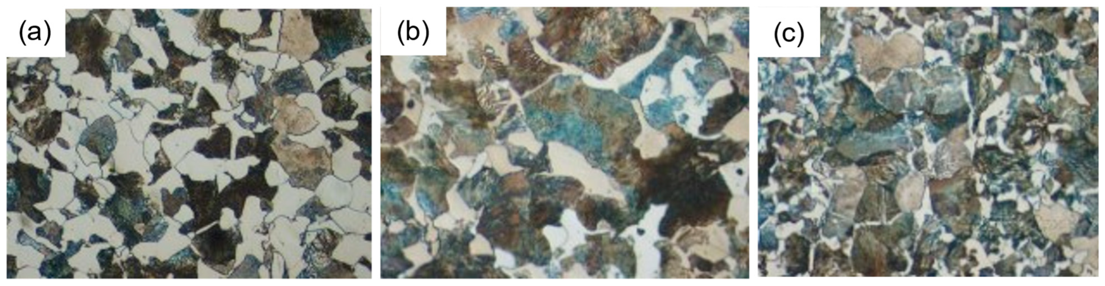
As seen in Figure 1a,b, once the steel undergoes an annealing heat treatment, a crystalline structure is obtained, revealing two distinctive zones. One zone is characterized by ferrite, appearing as a whitish matrix, while the other zone appears darker with a lamellar constituent, indicating the presence of pearlite. The normalizing heat treatment results in a similar microstructure, albeit with finer constituents, as shown in Figure 1c. 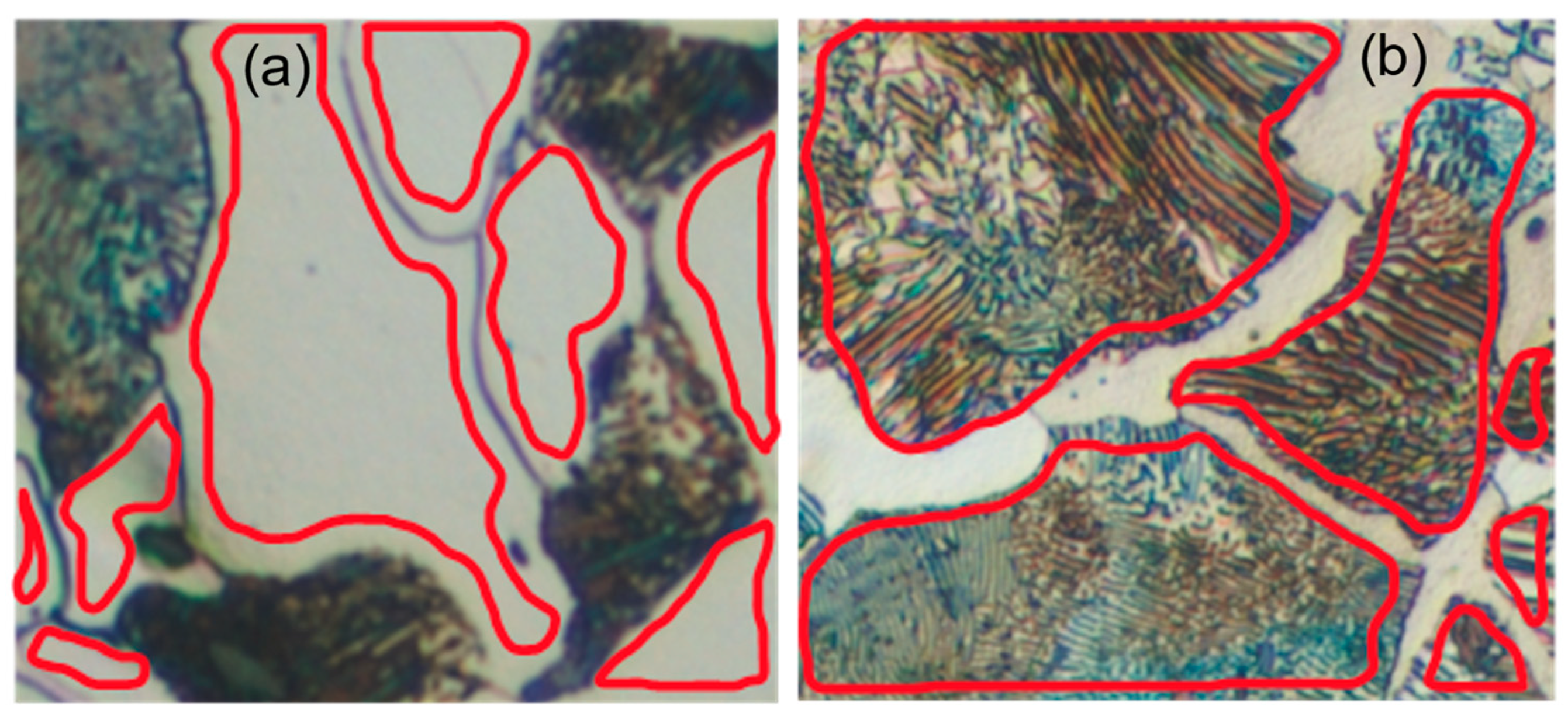Figure 2 provides a detailed depiction of these constituents. As observed in Figure 2b, the pearlite consists of alternating fine bands of ferrite and cementite, maintaining a dark aspect, as mentioned earlier.

2.2. Image Preprocessing

In the preprocessing stage of the segmentation deep learning experiment carried out in this work, a comprehensive approach was implemented to enhance the quality and diversity of the dataset. This involved the initial creation of masks using specialized software, followed by a thorough data augmentation process. ImageJ, with its trainable Weka segmentation plugin, was utilized for the creation of masks [22,23]. This allowed for the creation of masks, outlining specific regions of interest within the steel microstructure images. Manual annotations made by the authors guided the algorithm in learning the features necessary for accurate segmentation. The annotations of the pearlite areas have been manually performed on two of the original images for each sample. Subsequently, the trainable Weka segmentation option has been applied to the rest of the images to automate the generation of masks since manual mask generation is a time-consuming process and prone to errors. Thus, by using the ImageJ segmentation assistant, the quality of the masks was improved, and the processing time was reduced. Nevertheless, the authors reviewed each generated mask, making adjustments to images containing any errors.

The trainable classifier employed for mask creation was based on the Random Forest algorithm. Configured with 200 decision trees, this algorithm demonstrated robustness in handling the complexity of steel micrography images. The training process involved feeding the algorithm with the manually annotated masks, allowing it to learn and generalize patterns within the dataset. Following the initial mask creation and classifier training, a data augmentation step was introduced to enhance the dataset’s diversity. This involved applying various transformations such as rotation, scaling, and flipping to the original 34 steel micrography images. The augmented dataset served to increase the model’s ability to generalize across a broader range of microstructural variations.

Each original image captured by the optical microscope has a resolution of 2080 × 1542 pixels. For the execution of the experiments, we have chosen to use images of 224 × 224 pixels. This choice is based on various practical and efficiency considerations. Smaller images demand fewer computational resources for both training and inference. The utilization of 224 × 224 images enables the model to execute more rapidly. Furthermore, for the transfer learning from pretrained models utilized in the experiments, such as ResNet50, ResNet18, or MobileNetV2, these models are often trained on massive datasets with specific image sizes. Employing the same image size during both training and inference eases the transfer of knowledge from pretrained models, as the initial layers are tailored to that size. It is important to note that although 224 × 224 pixels is a commonly used size, it is not a strict constraint. The image size can be adjusted to conduct experiments with a different set of images, but it might be necessary to adjust other model parameters and, in some cases, retrain the model to accommodate the new input size.

For data augmentation, each original image and mask were cropped into 54 images of size 224 × 224 pixels. Subsequently, rotations of 90°, 180°, and 270° were applied to the cropped images, resulting in 216 images for each original image. This process yielded a final dataset of 7344 images. These images were distributed randomly, with 70% allocated for training data, 20% for validation data, and 10% for the test data.

Taking into consideration the information provided before, an example of the result of the cropping and rotating images can be appreciated in Figure 3. The masking process intended to isolate the ferrite areas contained in the images can also be observed.

After the preprocessing stage was completed, the model creation phase was initiated. This involved training various segmentation models to identify important features in the preprocessed dataset. Using the enriched dataset, different model setups and methods were experimented with. The aim was to determine which approach worked best for accurately outlining the steel microstructure images. In the following section, the training process details and metrics are described.

2.3. Segmentation Model Training

In executing the experiments, various segmentation networks were employed to establish a comparative analysis and identify the most suitable one for the context of microstructures in steels subjected to an annealing heat treatment. The segmentation networks utilized include U-Net [24], SegNet [25], and DeepLabV3+ [26]. Diverse pre-trained backbones, such as ResNet18, ResNet50, and MobileNetV2, were employed for the latter.

The same algorithm has been applied to all networks. Initially, each model undergoes training using the selected images for training and validation. Once the model is generated, it is applied to the test images, subsequently obtaining various metrics [27] that facilitate result analysis. In Appendix A, comprehensive details regarding each layer within the architectures of the segmentation networks utilized are presented in tabular form. The description of the networks employed in the experiments is provided next.

2.3.1. U-Net

U-Net is commonly used in the context of semantic image segmentation, and its effectiveness in capturing both global context and fine details makes it particularly well-suited for tasks such as medical image segmentation and satellite image analysis, and it is also employed for the segmentation of materials microstructures [28,29]. U-Net is characterized by a U-shaped architecture with an encoder–decoder structure and skip connections. The encoder, on the left side of the U, consists of down-sampling layers that capture hierarchical features from the input image. The decoder, on the right side, involves up-sampling layers and skip connections that preserve high-resolution details and aid in precise localization. Skip connections connect corresponding encoder and decoder stages, facilitating the retention of spatial information. The bottleneck at the base of the U combines abstract features from the encoder with detailed spatial information from the decoder.

In the conducted experiments with U-Net, the bias term of all convolutional layers is initialized to zero. Additionally, the convolution layer weights in the encoder and decoder subnetworks are initialized using the ‘He’ weight initialization method [30]. The encoder–decoder has a depth of 3, resulting in a U-Net comprising 46 layers with 48 connections. The most relevant hyperparameters configured for training include the Adam optimizer, a learning rate of 0.001, L2 regularization, and a maximum number of epochs set to 2. Experiments were conducted by increasing the number of epochs, yet substantial improvements were not achieved; instead, there was an increase in computational time. The loss layer utilizes cross-entropy loss to quantify the disparity between the predicted values and their corresponding actual data. The formula is expressed as follows in Equation (1).

$$\mathrm{l}\mathrm{o}\mathrm{s}\mathrm{s}=-\frac{1}{\mathrm{N}}\sum _{\mathrm{n}=1}^{\mathrm{N}}\sum _{\mathrm{i}=1}^{\mathrm{K}}{\mathrm{w}}_{\mathrm{i}}{\mathrm{t}}_{\mathrm{n}\mathrm{i}}\ln {\mathrm{y}}_{\mathrm{n}\mathrm{i}}$$

(1)

Here, N represents the number of samples, K is the number of classes, w_i denotes the weight for class i, t_ni is the indicator of whether the nth sample belongs to the ith class, and y_ni represents the output for sample n for class i.

2.3.2. SegNet

SegNet [31] is a convolutional neural network architecture tailored for semantic image segmentation. Its distinctive features include a conventional encoder–decoder structure, where the encoder captures hierarchical features, and the decoder reconstructs the segmented output through up-sampling layers. Notably, SegNet utilizes max-pooling indices from the encoder during decoding to recover spatial information lost during down-sampling, contributing to accurate segmentation. The network leverages feature maps from the encoder for precise localization. Employing a class-specific softmax activation in the final layer enables pixel-wise classification. Although SegNet lacks skip connections between the encoder and decoder, its design, particularly the incorporation of pooling indices, makes it well-suited for tasks demanding detailed pixel-wise segmentation.

In this study, the segmentation experiments have utilized the SegNet architecture in conjunction with VGG16 [32,33]. In this context, VGG16 plays a role as a feature extractor, capturing high-level semantic information from the input images. It complements the segmentation capabilities of SegNet, contributing to an enhanced overall performance of the segmentation model.

2.3.3. DeepLabV3+

The segmentation models were built by integrating the DeepLabV3+ architecture with various pre-trained backbones, including ResNet50, ResNet18 [34], and MobileNetV2 [35]. This diverse combination harnesses the strengths of DeepLabV3+ for pixel-wise segmentation and different backbone architectures for feature extraction. The models were trained using an augmented dataset, integrating insights obtained from the Random Forest classifier.

In Figure 4, a schematic representation of the DeepLabV3+ architecture is shown. The model employs a pretrained backbone (ResNet50, ResNet18 and MobileNetv2) for feature extraction. The Atrous Spatial Pyramid Pooling (ASPP) module is employed to capture multi-scale contextual information. The subsequent decoder, featuring skip connections, refines and up-samples the features to produce a high-resolution semantic segmentation map. This architecture provides detailed pixel-wise predictions for accurate object recognition in images.

2.4. Training Parameters, Metrics and Other Details

The training process involved optimizing various parameters, including learning rates, batch sizes, and epochs. A validation set was used to monitor the model’s performance and prevent overfitting.

When conducting experiments, identical training parameters were chosen to ensure a more faithful comparison of results. Adam optimizer with a learning rate of 0.001 and a maximum number of epochs set to 3 were selected. Additionally, the ‘Validation Patience’ parameter was set to 4 to avoid unnecessary computation. All the aforementioned information is summarized in

Table 2. Training parameters and network information.

Network	Optimizer	Learning Rate	Max Epochs	Batch Size	Trainable Parameters	Layers
U-Net	Adam	0.001	3	32	7,697,410	46
SegNet				16	29,444,166	91
DeepLabv3+ (Resnet50)				32	43,980,180	206
DeepLabv3+ (Resnet18)					20,607,636	100
DeepLabv3+ (MobileNet)					6,784,276	186

, which compiles essential data regarding the networks for computational time considerations.

To evaluate the performance of the segmentation models, various metrics were employed. Accuracy measures the proportion of correctly classified pixels to the total number of pixels in each class, as defined by the ground truth, and its score is calculated using Equation (2), where TP represents true positives, and FN represents false negatives. Mean Accuracy, computed as the average Accuracy of all classes across all images, provides an aggregate assessment of model performance. Global Accuracy, on the other hand, considers the ratio of correctly classified pixels, irrespective of class, to the total number of pixels.

$$\mathrm{A}\mathrm{c}\mathrm{c}\mathrm{u}\mathrm{r}\mathrm{a}\mathrm{c}\mathrm{y}\mathrm{ }\mathrm{s}\mathrm{c}\mathrm{o}\mathrm{r}\mathrm{e}=\frac{\mathrm{T}\mathrm{P}}{\mathrm{T}\mathrm{P}+\mathrm{F}\mathrm{N}}$$

(2)

Additionally, the Boundary F1 (BF) score, known as the BF Score, evaluates the alignment between predicted boundaries and true boundaries. Calculated using Equation (3), precision assesses the accuracy of the predicted boundaries, while recall gauges the model’s ability to capture true boundaries. A higher BF score indicates better agreement between predicted and true boundaries. The Mean BF Score offers an aggregate measure of boundary prediction performance across all classes and images.

$$\mathrm{B}\mathrm{F}\mathrm{ }\mathrm{s}\mathrm{c}\mathrm{o}\mathrm{r}\mathrm{e}\mathrm{ }=\mathrm{ }\frac{2\mathrm{ }\times \mathrm{ }\mathrm{p}\mathrm{r}\mathrm{e}\mathrm{c}\mathrm{i}\mathrm{s}\mathrm{i}\mathrm{o}\mathrm{n}\mathrm{ }\times \mathrm{r}\mathrm{e}\mathrm{c}\mathrm{a}\mathrm{l}\mathrm{l}}{\mathrm{p}\mathrm{r}\mathrm{e}\mathrm{c}\mathrm{i}\mathrm{s}\mathrm{i}\mathrm{o}\mathrm{n}\mathrm{ }+\mathrm{ }\mathrm{r}\mathrm{e}\mathrm{c}\mathrm{a}\mathrm{l}\mathrm{l}}$$

(3)

Furthermore, the Intersection over Union (IoU) score assesses the ratio of correctly classified pixels to the total number of ground truth and predicted pixels in each class. The IoU score is computed using Equation (4), where TP represents true positives, FP represents false positives, and FN represents false negatives. The Mean IoU provides an average IoU score across all classes and images, offering insights into the overall segmentation accuracy of the model.

$$\mathrm{I}\mathrm{o}\mathrm{U}\mathrm{ }\mathrm{s}\mathrm{c}\mathrm{o}\mathrm{r}\mathrm{e}\mathrm{ }=\mathrm{ }\frac{\mathrm{T}\mathrm{P}}{\mathrm{T}\mathrm{P}+\mathrm{F}\mathrm{P}+\mathrm{F}\mathrm{N}}$$

(4)

The trained segmentation models were evaluated on a separate test set of steel micrograph images not seen during training. The metrics used for the evaluation of the models have been previously specified.

All experiments were conducted on a robust computing system equipped with an Intel(R) Core(TM) i7-5930K CPU @ 3.50 GHz, DIMM 64 GB RAM, and an NVIDIA^® GEFORCE RTX 3080 (10 GB). MATLAB^® (R2023b, The MathWorks, Inc., Natick, MA, USA) was utilized for coding and generating segmentation models, and ImageJ was employed for mask creation, guaranteeing a stable and reproducible computational environment. All codes performed for this research are available upon request.

3. Results

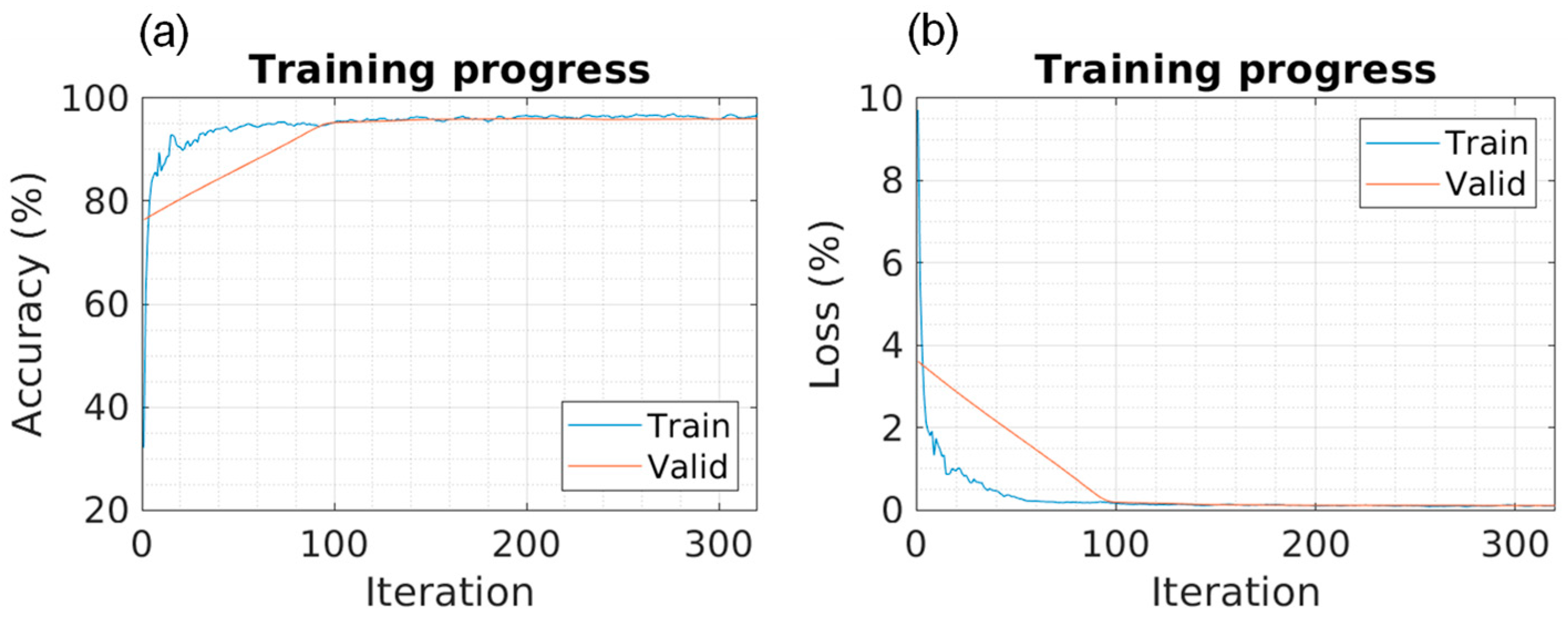
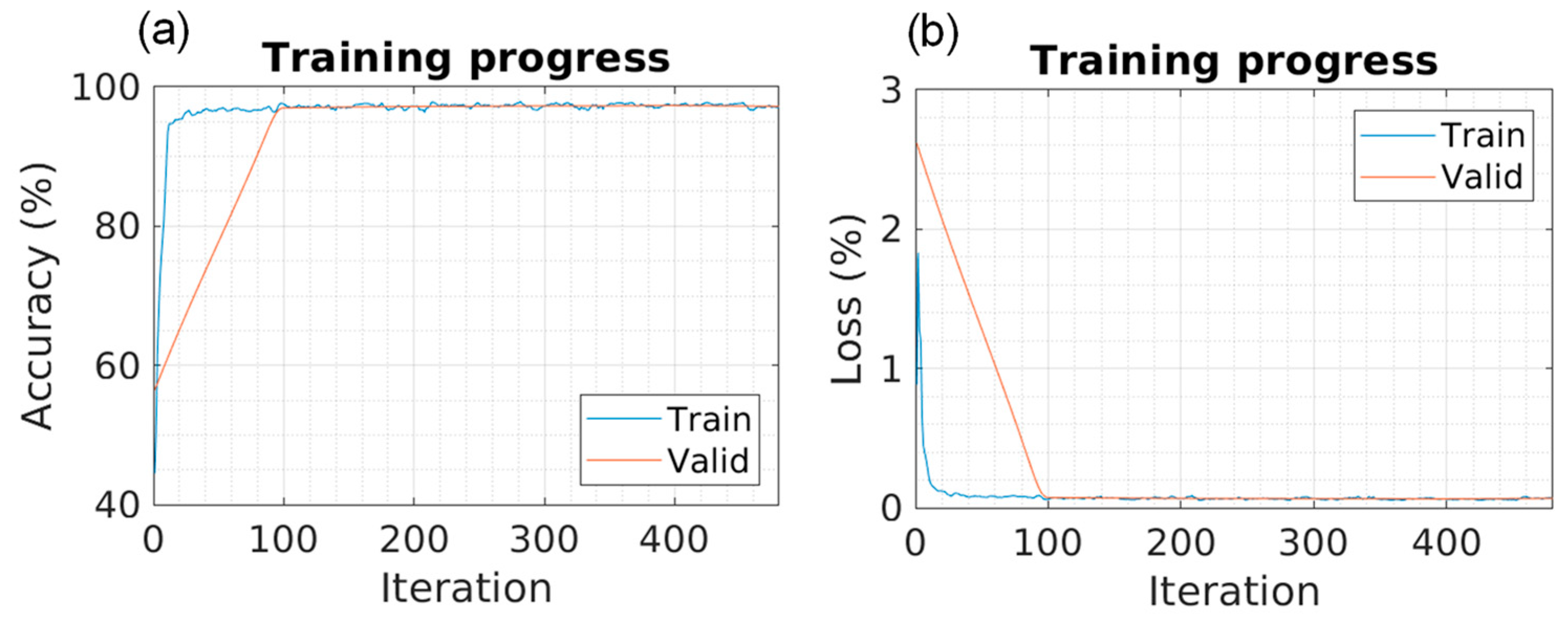
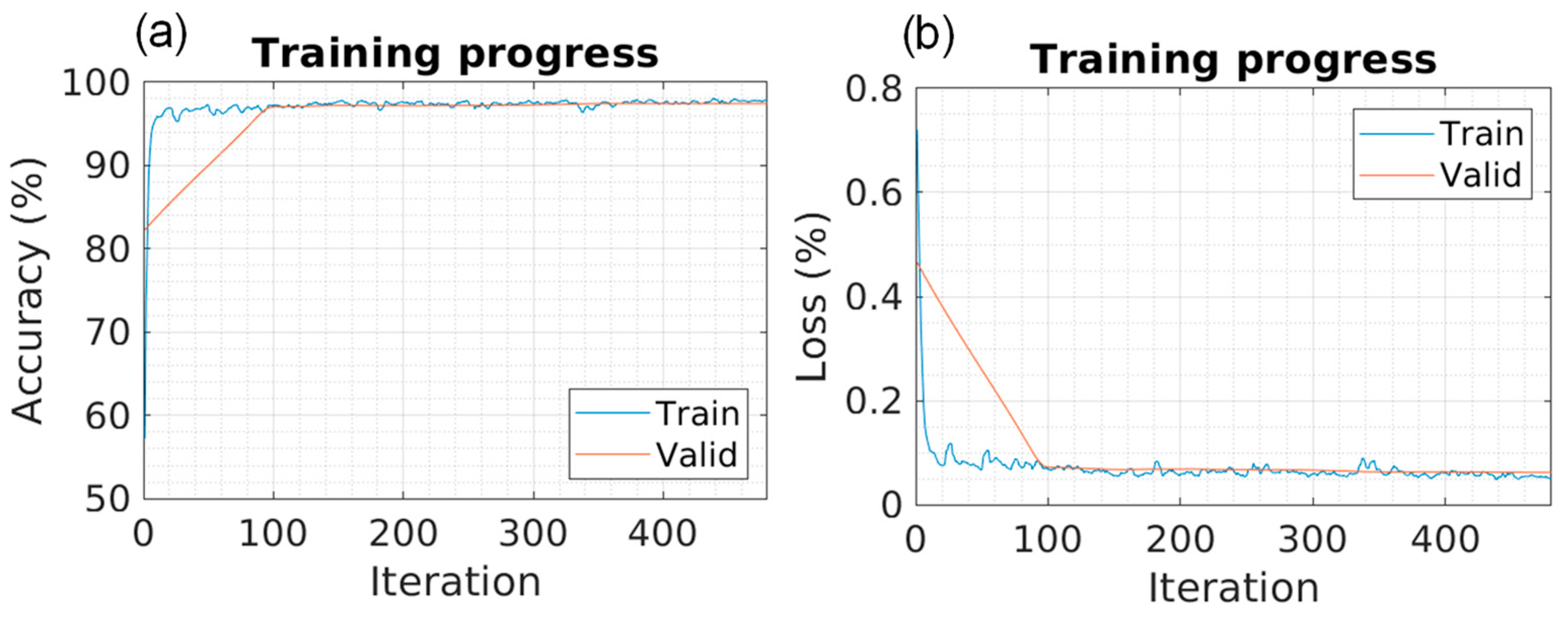
Five different models were trained using 5141 training images and 1469 validation images. The training results are presented in

Table 3. Training results (LR = 0.001) (bold numbers represent the maximum values).

Model	Training Accuracy (%)	Training Loss	Final Validation Accuracy (%)	Final Validation Loss	Output Network Iteration	Time Elapsed (hh:mm:ss)
U-Net	95.874	0.128	96.553	0.095	320	00:06:50
DeepLabv3+resn50	97.185	0.068	97.485	0.060	480	00:08:14
DeepLabv3+resn18	97.229	0.068	97.177	0.071	480	00:04:49
DeepLabv3+mobn	97.379	0.063	97.969	0.050	480	00:07:41
SegNet	95.359	0.236	96.773	0.169	963	00:20:23

, and the training progress can be observed in Figure 5, Figure 6, Figure 7, Figure 8 and Figure 9 for each of the models. The progression of both accuracy and the loss function is depicted.

The model was then applied to 734 test images that it had not seen previously. The results of the test experiments are included in

Table 4. Test image metrics (bold numbers represent the maximum values).

Model	Global Accuracy	Mean Accuracy	Mean IOU	Weighted IOU	Mean BF Score
U-Net	0.9667	0.9551	0.9202	0.9359	0.8578
DeepLabv3+ResNet50	0.9757	0.9722	0.9418	0.9529	0.8798
DeepLabv3+ResNet18	0.9725	0.9717	0.9349	0.9472	0.8471
DeepLabv3+MobNetv2	0.9802	0.9743	0.9521	0.9614	0.9149
SegNet	0.9675	0.9596	0.9229	0.9377	0.8127

, which displays the usual metrics for segmentation problems. Additionally, the confusion matrices are shown in Figure 10. It can be inferred that the DeepLabv3+ model with MobileNetv2 achieves a performance improvement, though only slightly surpassing the other networks that also accurately solve the segmentation problem.

To visually explore the results, two test images were utilized, and each was processed by every trained model. These images are depicted in Figure 11. The segmentation performed by each model can be observed for comparison with the original sample, as well as with the mask or ground truth generated during data preprocessing before training. The objective is to distinguish between the two microconstituents: ferrite as the matrix element represented by the lighter zone in the micrograph and pearlite composed of alternating layers of cementite and ferrite. It is crucial to emphasize that the ferrite constituting the pearlite should not be segmented together with the ferrite, forming the matrix of the microstructure.

In the training phase, it can be observed that the SegNet model requires more iterations and, consequently, more computational time to achieve maximum accuracy, as depicted in Figure 6, exceeding more than twice the others. However, its final training accuracy does not differ significantly from the rest, trailing only by a couple of percentage points compared to DeepLabv3+, which yields the best results. This increased number of iterations is due to the reduction in MiniBatchSize to 16 samples for SegNet, compared to the MiniBatchSize of 32 samples used for the other networks. Notably, when employing a MiniBatchSize of 32 samples, the performance of SegNet decreases to approximately 91% to 93%, emphasizing the need to reduce the MiniBatchSize to 16 for optimal performance. Despite the longer training time associated with the reduced MiniBatchSize, SegNet’s final accuracy remains competitive, showcasing its ability to achieve high performance even with a smaller batch size. 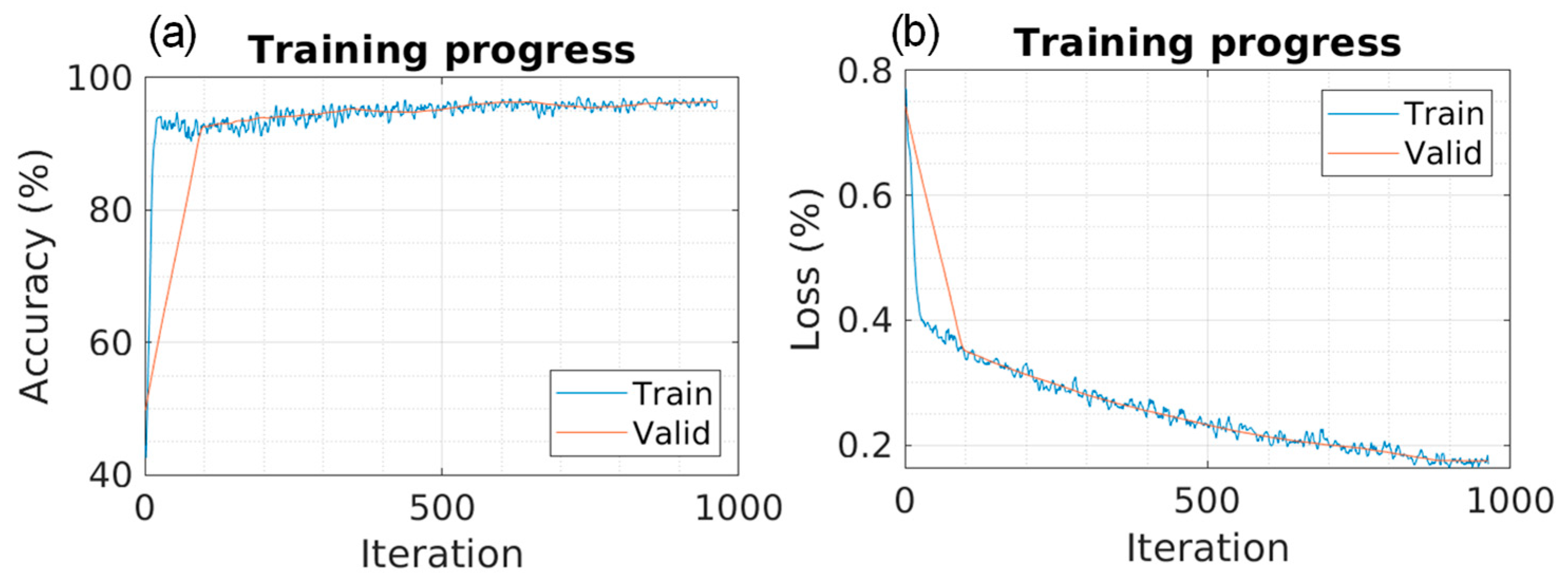As shown in Figure 7, Figure 8 and Figure 9 achieving maximum accuracy during training requires only a few iterations for DeepLabv3+ segmentation networks. The encoder that leads to the shortest training time is ResNet18, which has the fewest layers among the three. However, MobileNetV2 exhibits slightly superior results to the other networks, achieving excellent scores in all metrics as indicated in Table 4.

During the training process of the segmentation model, anomalies or irregularities that might occur in individual images are likely to diminish or be addressed as the model learns from a diverse set of images. The learning process, driven by probabilities, helps the model to generalize and effectively segment objects or regions of interest in images, even in cases where there might be variations or anomalies in the data. In this case, the model might not learn extensively about these imperfections due to their limited occurrence in the training data.

4. Discussion

Different random test samples were selected for segmentation using the obtained models. The accuracy and loss values in Figure 5, Figure 6, Figure 7, Figure 8 and Figure 9 are obtained during training. The overall values, as shown in Table 4, are calculated based on test images that the model had not previously seen. These test values closely resemble those observed during training, indicating that no “overfitting” has occurred in any of the models.

Algorithms with lower loss rates and higher accuracy during training may demonstrate superior generalization performance on unseen data, resulting in higher final accuracy.

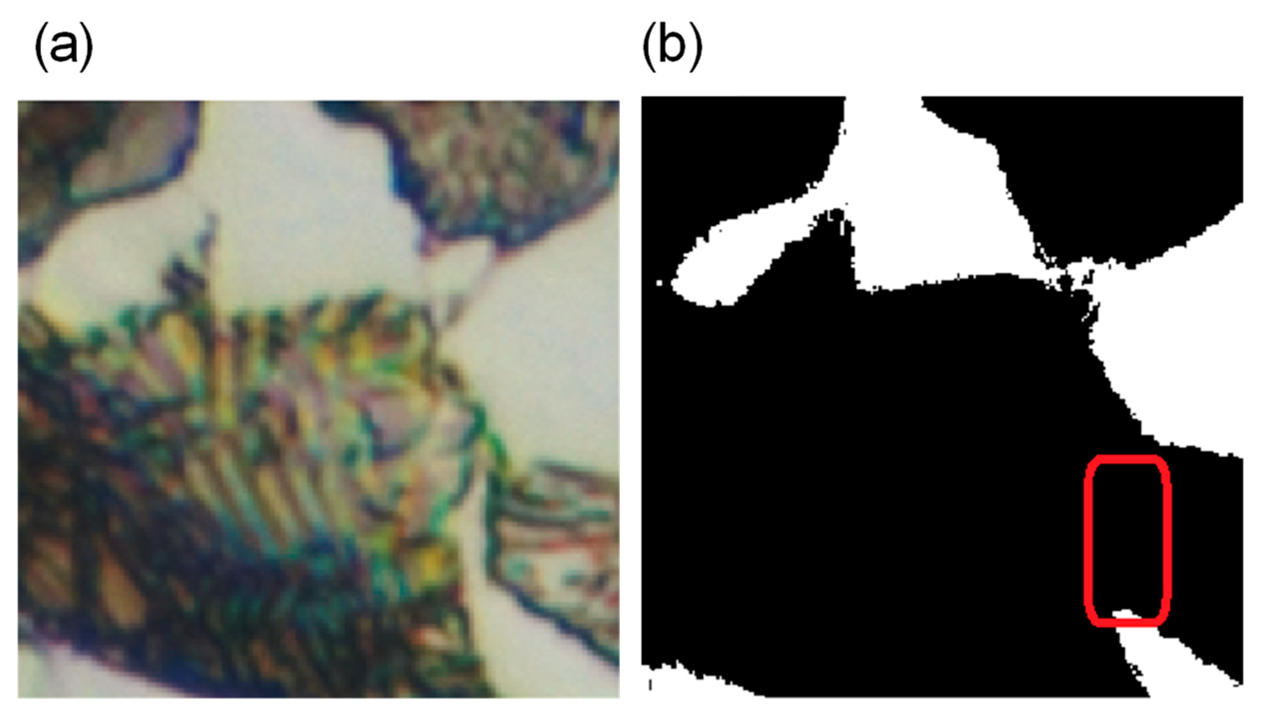
In Figure 11 (segmented samples), a comparison of 224 × 224 images of annealed steel is presented, highlighting the region considered as perlite in green hues and the matrix or ferrite, which appears light in the original image and violet in the segmented image. The grayscale image corresponds to the mask generated during data preprocessing. Although the results are very similar, subtle differences can be perceived. It is important to note that some masks were created manually, while the rest underwent preprocessing using a Random Forest algorithm with WEKA software (ImageJ2-Figi GPLv3+, Waikato University, New Zeland). This process may have introduced errors in pixel annotation in some masks, causing the model to learn from imperfect images. As shown in microstructure A, there is an error in the bottom right part of the mask (slightly pointed area), Figure 12a, where the ferrite zone connecting with the one in the top right has not been completely obtained. This flaw is highlighted in red in Figure 12b. This error has also been transferred to the training models, which consequently failed to detect the ferrite in that zone. However, a slight improvement in the segmented area compared to the mask is noticeable. Similarly, in image B, impurities can be observed on the ferrite area (two dots on the left side), which were also transferred to the training dataset. In this case, models like DeepLabv3 with ResNet50-18 have effectively eliminated these impurities during the segmentation process.

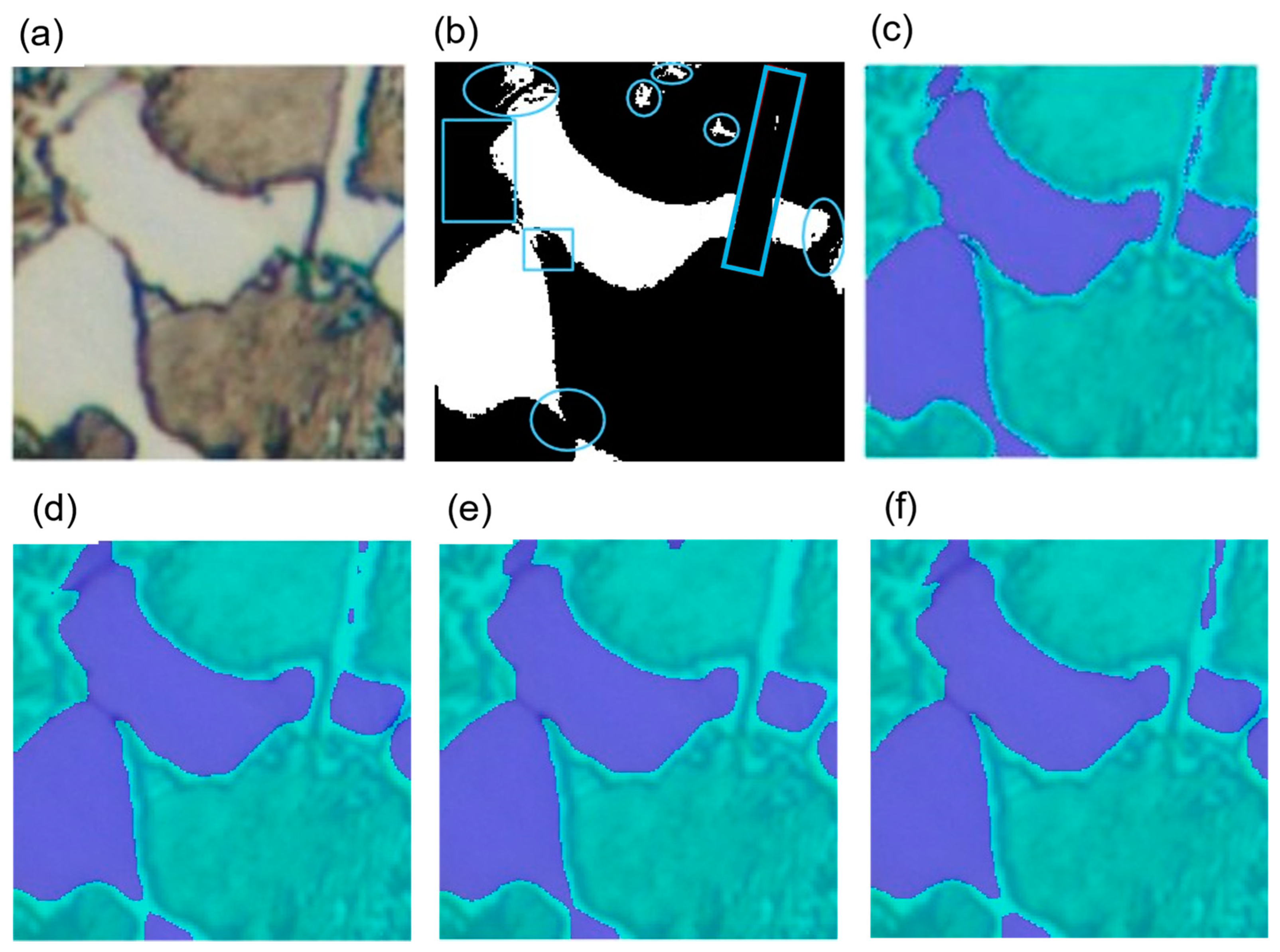
As shown in Figure 13, another test sample was selected, and errors in the identification of ferrite and perlite were marked on the corresponding mask image. The segmented images by the models demonstrate improvement over the mask created for training. We can observe that in the original image, it is difficult to appreciate the laminar structure of perlite. Although ferrite, as the matrix element of the microstructure, should be easily detected due to its more uniform and clear texture, the models encounter issues in some areas, such as the band in Figure 13b, which is indicated in the red rectangular area. Considering perlite as alternating layers of ferrite and cementite, the thickness of this bright band between two darker zones causes the models to interpret that area as perlite. The models with DeepLabv3+/MobileNetv2, shown in Figure 13f and, to some extent, U-Net, manage to enhance segmentation in that specific area.

5. Conclusions

This study investigates the identification of microconstituents, specifically ferrite and perlite, in optical metallographic images of steels using deep learning networks specialized in image segmentation problems. The work encompasses challenging tasks, particularly in obtaining and preparing the images. While other studies often concentrate on detecting various microconstituents using electron microscopy, where differences are typically more pronounced, our focus is on optical images. As the core of this study is grounded in optical images, a preliminary investigation has been undertaken on microconstituents derived from annealing heat treatments.

Segmenting distinct and clearly identifiable textures, such as perlite and ferrite, could be approached using classical algorithms with the application of conventional computer vision filters or classical machine learning techniques. However, in other studies conducted by the authors, it has been confirmed that the application of deep learning techniques to steel metallographic images enhances the metrics compared to classical machine learning algorithms. The advantage of approaching the study through deep learning is the creation of models that can be integrated into more general models in the future through transfer learning or model ensemble, thereby forming a superior structure.

References

1. Larmuseau, M.; Sluydts, M.; Theuwissen, K.; Duprez, L.; Dhaene, T.; Cottenier, S. Race against the Machine: Can Deep Learning Recognize Microstructures as Well as the Trained Human Eye? Scr. Mater. 2021, 193, 33–37. [Google Scholar] [CrossRef]
2. DeCost, B.L.; Francis, T.; Holm, E.A. Exploring the Microstructure Manifold: Image Texture Representations Applied to Ultrahigh Carbon Steel Microstructures. Acta Mater. 2017, 133, 30–40. [Google Scholar] [CrossRef]
3. Gupta, S.; Banerjee, A.; Sarkar, J.; Kundu, M.; Sinha, S.K.; Bandyopadhyay, N.R.; Ganguly, S. Modelling the Steel Microstructure Knowledge for In-Silico Recognition of Phases Using Machine Learning. Mater. Chem. Phys. 2020, 252, 123286. [Google Scholar] [CrossRef]
4. Wang, J.; Fa, Y.; Tian, Y.; Yu, X. A Machine-Learning Approach to Predict Creep Properties of Cr–Mo Steel with Time-Temperature Parameters. J. Mater. Res. Technol. 2021, 13, 635–650. [Google Scholar] [CrossRef]
5. Yucel, B.; Yucel, S.; Ray, A.; Duprez, L.; Kalidindi, S.R. Mining the Correlations between Optical Micrographs and Mechanical Properties of Cold-Rolled HSLA Steels Using Machine Learning Approaches. Integr. Mater. Manuf. Innov. 2020, 9, 240–256. [Google Scholar] [CrossRef]
6. Wang, Z.-L.; Adachi, Y. Property Prediction and Properties-to-Microstructure Inverse Analysis of Steels by a Machine-Learning Approach. Mater. Sci. Eng. A Struct. Mater. 2019, 744, 661–670. [Google Scholar] [CrossRef]
7. Larmuseau, M.; Theuwissen, K.; Lejaeghere, K.; Duprez, L.; Dhaene, T.; Cottenier, S. Towards Accurate Processing-Structure-Property Links Using Deep Learning. Scr. Mater. 2022, 211, 114478. [Google Scholar] [CrossRef]
8. Muñoz-Rodenas, J.; García-Sevilla, F.; Coello-Sobrino, J.; Martínez-Martínez, A.; Miguel-Eguía, V. Effectiveness of Machine-Learning and Deep-Learning Strategies for the Classification of Heat Treatments Applied to Low-Carbon Steels Based on Microstructural Analysis. Appl. Sci. 2023, 13, 3479. [Google Scholar] [CrossRef]
9. Luengo, J.; Moreno, R.; Sevillano, I.; Charte, D.; Peláez, A.; Fernández, M.; Herrera, F. A tutorial on the segmentation of metallographic images: Taxonomy, new MetalDAM dataset, deep learning-based ensemble model, experimental analysis and challenges. Inf. Fusion 2022, 78, 232–253. [Google Scholar] [CrossRef]
10. Bulgarevich, D.; Tsukamoto, S.; Kasuya, T.; Demura, M.; Watanabe, M. Pattern recognition with machine learning on optical microscopy images of typical metallurgical microstructures. Sci. Rep. 2018, 8, 2078. [Google Scholar] [CrossRef]
11. Bachmann, B.; Müller, M.; Britz, D.; Durmaz, A.; Ackermann, M.; Shchyglo, O.; Staudt, T.; Mücklich, F. Efficient reconstruction of prior austenite grains in steel from etched light optical micrographs using deep learning and annotations from correlative microscopy. Front. Mater. 2022, 9, 1033505. [Google Scholar] [CrossRef]
12. Han, Y.; Li, R.; Yang, S.; Chen, Q.; Wang, B.; Liu, Y. Center-environment feature models for materials image segmentation based on machine learning. Sci. Rep. 2022, 12, 12960. [Google Scholar] [CrossRef]
13. Kim, H.; Inoue, J.; Kasuya, T. Unsupervised microstructure segmentation by mimicking metallurgists’ approach to pattern recognition. Sci. Rep. 2020, 10, 17835. [Google Scholar] [CrossRef]
14. Breumier, S.; Martinez, T.; Frincu, B.; Gey, N.; Couturier, A.; Loukachenko, N.; Aba-perea, P.E.; Germain, L. Leveraging EBSD data by deep learning for bainite, ferrite and martensite segmentation. Mater. Charact. 2022, 186, 111805. [Google Scholar] [CrossRef]
15. Chaurasia, N.; Jha, S.K.; Sangal, S. A Novel Training Methodology for Phase Segmentation of Steel Microstructures Using a Deep Learning Algorithm. Materialia 2023, 30, 101803. [Google Scholar] [CrossRef]
16. Liu, J.; Cao, G.; Wang, H.; Cui, C.; Liu, Z. Development of Intelligent Methodologies Perceiving Microstructure and Mechanical Properties of Hot Rolled Steels. Measurement 2023, 221, 113526. [Google Scholar] [CrossRef]
17. Azimi, S.M.; Britz, D.; Engstler, M.; Fritz, M.; Mücklich, F. Advanced Steel Microstructural Classification by Deep Learning Methods. Sci. Rep. 2018, 8, 2128. [Google Scholar] [CrossRef]
18. Martinez Ostormujof, T.; Purushottam Raj Purohit, R.R.P.; Breumier, S.; Gey, N.; Salib, M.; Germain, L. Deep Learning for Automated Phase Segmentation in EBSD Maps. A Case Study in Dual Phase Steel Microstructures. Mater. Charact. 2022, 184, 111638. [Google Scholar] [CrossRef]
19. Xie, L.; Li, W.; Fan, L.; Zhou, M. Automatic Identification of the Multiphase Microstructures of Steels Based on ASPP-FCN. Steel Res. Int. 2023, 94, 202200204. [Google Scholar] [CrossRef]
20. Ma, X.; Yu, Y. Training Tricks for Steel Microstructure Segmentation with Deep Learning. Processes 2023, 11, 3298. [Google Scholar] [CrossRef]
21. Bihani, A.; Daigle, H.; Santos, J.E.; Landry, C.; Prodanović, M.; Milliken, K. MudrockNet: Semantic Segmentation of Mudrock SEM Images through Deep Learning. Comput. Geosci. 2022, 158, 104952. [Google Scholar] [CrossRef]
22. Arganda-Carreras, I.; Kaynig, V.; Rueden, C.; Eliceiri, K.W.; Schindelin, J.; Cardona, A.; Seung, H.S. Trainable Weka Segmentation: A machine learning tool for microscopy pixel classification. Bioinformatics 2017, 33, 2424–2426. [Google Scholar] [CrossRef] [PubMed]
23. Somasundaram, E.; Kaufman, R.; Brady, S. Advancements in Automated Tissue Segmentation Pipeline for Contrast-Enhanced CT Scans of Adult and Pediatric Patients. In Proceedings of the SPIE Medical Imaging, Orlando, FL, USA, 13–16 February 2017; Armato, S.G., Petrick, N.A., Eds.; SPIE: Bellingham, WA, USA, 2017. [Google Scholar]
24. Ronneberger, O.; Fischer, P.; Brox, T. U-Net: Convolutional Networks for Biomedical Image Segmentation. In Proceedings of the Medical Image Computing and Computer-Assisted Intervention (MICCAI) 2015, Munich, Germany, 5–9 October 2015; Volume 9351, pp. 234–241. [Google Scholar]
25. Badrinarayanan, V.; Kendall, A.; Cipolla, R. SegNet: A Deep Convolutional Encoder-Decoder Architecture for Image Segmentation. IEEE Trans. Pattern Anal. Mach. Intell. 2015, 39, 2481–2495. [Google Scholar] [CrossRef] [PubMed]
26. Chen, L.-C.; Zhu, Y.; Papandreou, G.; Schroff, F.; Adam, H. Encoder-Decoder with Atrous Separable Convolution for Semantic Image Segmentation. In Proceedings of the Computer Vision—ECCV 2018, Munich, Germany, 8–14 September 2018; Springer International Publishing: Cham, Switzerland, 2018; pp. 833–851, ISBN 9783030012335. [Google Scholar]
27. Csurka, G.; Larlus, D.; Perronnin, F. What is a good evaluation measure for semantic segmentation? In Proceedings of the British Machine Vision Conference, Bristol, UK, 9–13 September 2013; pp. 32.1–32.11. [Google Scholar]
28. Swain, B.R.; Cho, D.; Park, J.; Roh, J.-S.; Ko, J. Complex-Phase Steel Microstructure Segmentation Using UNet: Analysis across Different Magnifications and Steel Types. Materials 2023, 16, 7254. [Google Scholar] [CrossRef] [PubMed]
29. Han, Y.; Li, R.; Wang, B.; Ruan, L.; Chen, Q. A Pseudo-Labeling Based Weakly Supervised Segmentation Method for Few-Shot Texture Images. Expert Syst. Appl. 2024, 238, 122110. [Google Scholar] [CrossRef]
30. He, K.; Zhang, X.; Ren, S.; Sun, J. Delving Deep Into Rectifiers: Surpassing Human-Level Performance on ImageNet Classification. In Proceedings of the IEEE International Conference on Computer Vision, Santiago, Chile, 7–13 December 2015; pp. 1026–1034. [Google Scholar]
31. Ajioka, F.; Wang, Z.-L.; Ogawa, T.; Adachi, Y. Development of High Accuracy Segmentation Model for Microstructure of Steel by Deep Learning. ISIJ Int. 2020, 60, 954–959. [Google Scholar] [CrossRef]
32. Simonyan, K.; Zisserman, A. Very Deep Convolutional Networks for Large-Scale Image Recognition. arXiv 2014, arXiv:1409.1556v6. [Google Scholar]
33. Russakovsky, O.; Deng, J.; Su, H.; Krause, J.; Satheesh, S.; Ma, S.; Huang, Z.; Karpathy, A.; Khosla, A.; Bernstein, M.; et al. ImageNet Large Scale Visual Recognition Challenge. Int. J. Comput. Vis. IJCV 2015, 115, 211–252. [Google Scholar] [CrossRef]
34. He, K.; Zhang, X.; Ren, S.; Sun, J. Deep Residual Learning for Image Recognition. In Proceedings of the 2016 IEEE Conference on Computer Vision and Pattern Recognition (CVPR), Las Vegas, NV, USA, 27–30 June 2016; IEEE: Piscataway, NJ, USA, 2016; pp. 770–778. [Google Scholar]
35. Sandler, M.; Howard, A.; Zhu, M.; Zhmoginov, A.; Chen, L.-C. MobileNetV2: Inverted Residuals and Linear Bottlenecks. In Proceedings of the 2018 IEEE/CVF Conference on Computer Vision and Pattern Recognition, Salt Lake City, UT, USA, 18–23 June 2018; IEEE: Piscataway, NJ, USA, 2018; pp. 4510–4520. [Google Scholar]
Figure 1. Samples of C45E steel in an annealing state, (a,b) and normalizing; (c) reagent, Nital-1.
Applsci 14 02297 g001
Figure 2. Microconstituents corresponding to the C45E Steel (reagent Nital-1). The red contours correspond to ferrite (a) and pearlite (b) areas.
Applsci 14 02297 g002
Figure 3. Cropped and rotated sample images and masks with a resolution of 224 × 224 pixels.
Applsci 14 02297 g003
Figure 4. DeepLabV3+ and Resnet50 segmentation network architecture (adapted from [26]).
Applsci 14 02297 g004
Figure 5. Training progress of U-Net: (a) training and validation accuracy; (b) training and validation loss.
Applsci 14 02297 g005
Figure 6. Training progress of SegNet: (a) training and validation accuracy; (b) training and validation loss.
Applsci 14 02297 g006
Figure 7. Training progress of DeepLabv3+/ResNet50: (a) training and validation accuracy; (b) training and validation loss.
Applsci 14 02297 g007
Figure 8. Training progress of DeepLabv3+/ResNet18: (a) training and validation accuracy; (b) training and validation loss.
Applsci 14 02297 g008
Figure 9. Training progress of DeepLabv3+/MobileNetv2: (a) training and validation accuracy; (b) training and validation loss.
Applsci 14 02297 g009
Figure 10. Confusion Matrix: (a) U-Net, (b) SegNet, (c) DeepLabv3+/ResNet50, (d) DeepLabv3+/ResNet18, and (e) Mobilenetv2.
Applsci 14 02297 g010
Figure 11. Segmented samples. A and B correspond to two randomly selected samples.
Applsci 14 02297 g011
Figure 12. Detail of the error in mask production during preprocessing. (a) Image from test dataset; (b) mask. The red box indicates the lack of ferrite in the mask.
Applsci 14 02297 g012
Figure 13. U-Net, (a) test image sample, (b) mask of the sample, (c) semantic segmentation U-NET, (d) DeepLabv3+/ResNet50, (e) DeepLabv3+/ResNet18, and (f) Deeplabv3/MobileNetv2.
Applsci 14 02297 g013