
The Nonlinear and Threshold Effect of Built Environment on Ride-Hailing Travel Demand


College of Automobile and Traffic Engineering, Nanjing Forestry University, Nanjing 210037, China
*
Authors to whom correspondence should be addressed.
Appl. Sci. 2024, 14(10), 4072; https://doi.org/10.3390/app14104072
Submission received: 9 April 2024
/
Revised: 27 April 2024
/
Accepted: 4 May 2024
/
Published: 10 May 2024
Abstract
:While numerous studies have explored the correlation between the built environment and ride-hailing demand, few have assessed their nonlinear interplay. Utilizing ride-hailing order data and multi-source built environment data from Nanjing, China, this paper uses the machine learning method, eXtreme Gradient Boosting (XGBoost), combined with Shapley Additive exPlanations (SHAP) and Partial Dependence Plots (PDPs) to investigate the impact of built environment factors on ride-hailing travel demand, including their nonlinear and threshold effects. The findings reveal that dining facilities have the most significant impact, with a contribution rate of 30.75%, on predicting ride-hailing travel demand. Additionally, financial, corporate, and medical facilities also exert considerable influence. The built environment factors need to reach a certain threshold or within a certain range to maximize the impact of ride-hailing travel demand. Population density, land use mix, and distance to the subway station collectively influence ride-hailing demand. The results are helpful for TNCs to allocate network ride-hailing resources reasonably and effectively.
1. Introduction
Transportation Network Companies (TNCs) such as Uber, Lyft, and DiDi build service platforms based on Internet technology to match vehicles online and provide travel services for travelers in real time, also known as ride-hailing services. Amid the swift progress of information technology and the popularity of smartphones, ride-hailing as a shared travel mode has reduced passenger waiting time and improved travel efficiency, and is gradually becoming one significant mode of daily urban transportation [1]. The scale of ride-hailing users in China continues to expand, where the ride-hailing user base has surged to 453 million at the end of 2021. Although ride-hailing provides passengers with high accessibility services, research has shown that there is an alternative or complementary relationship between ride-hailing and transit [2,3]. Some researchers have found that ride-hailing has replaced traditional modes of transportation, leading to various issues including traffic congestion, increased energy consumption, and higher vehicle mileage, which in turn contribute to additional traffic pressure [4].
As a microscopic manifestation of urban spatial form, the built environment significantly influences travel patterns [5,6,7]. A multitude of scholars have scrutinized the nexus between the built environment and traffic travel, and have studied different models, including the metro [8,9], taxis [10,11,12], dockless bike-sharing [13,14] and private cars [15,16,17]. As a rising mode of travel, ride-hailing is gradually affecting the change in residents’ travel demand. The built environment factors also wield a significant influence on this phenomenon. In the pursuit of promoting green, low-carbon, and sustainable urban development, delving into the impact mechanism between the built environment and ride-hailing becomes imperative.
Researchers have discussed the relationship between the built environment and the demand for ride-hailing travel. Most of them start from the characteristics of spatial attributes, including spatial autocorrelation and spatial heterogeneity. Spatial autocorrelation effects are usually explained by spatial econometric models [18]. Geographically Weighted Regression (GWR) enhances regression accuracy by creating a local spatial weight matrix to estimate spatial variations [19]. The GWR and its variations are frequently utilized to investigate the spatial diversity in how the built environment influences ride-hailing travel demand [20,21,22]. On the one hand, these models assume that there is a linear or generalized linear relationship between the two, and the conclusions may have some deviations. On the other hand, the machine learning method possesses the advantage of not adhering to the assumption of linear relationships between variables in multivariate fitting, allowing for more flexible modeling of complex relationships, which helps find complex nonlinear relationships [23]. Based on this, contemporary research has started to explore the nonlinear impact of the built environment on travel behavior, and the threshold effect of the built environment can also be observed [9,24,25]. However, there are few studies on the nonlinear correlation and threshold effect amid the built environment and ride-hailing travel demand.
To address this gap, this study utilizes weekday ride-hailing travel data from Nanjing, China, and applies a machine learning method, XGBoost, to explore the complex relationship between the built environment and the ride-hailing travel demand, using the XGBoost model to identify the important built environment characteristics influencing ride-hailing travel demand. The SHAP summary plot and traditional PDPs are used to explain the threshold effect between the built environment and the ride-hailing service. It furnishes a foundation for TNCs to enhance their current ride-hailing service and has policy implications for how future urban land use and transportation strategies can effectively affect the ride-hailing service.
The remainder of this paper is structured as follows. Section 2 provides a review of research concerning the built environment’s influence on ride-hailing, with a particular focus on exploring the nonlinear relationship between influencing factors and travel behavior. Section 3 delineates the study area and outlines the pertinent variables involved. Section 4 introduces the modeling approach adopted in this study. Section 5 introduces the model estimation findings and analyzes them. Section 6 provides an overview of the primary research outcomes and suggests future avenues for investigation.
2. Literature Review
2.1. Impact of the Built Environment on Ride-Hailing
In recent years, ride-hailing services have become increasingly pivotal in the overall transportation system. Research on the key factors influencing ride-hailing trips has received widespread attention, including social demographics [26,27], user attitudes and preferences [28,29], built environment characteristics [20,21,22], and other factors such as weather conditions [26]. Among these, the urban built environment, as a crucial factor affecting residents’ travel behavior, is closely associated with ride-hailing trips. Built environment characteristics are commonly described using the “5Ds”: density, diversity, design, destination accessibility, and distance to transit [30,31]. This framework has now been expanded to “7Ds”, encompassing demand management and demographic factors.
Various aspects of the built environment, such as population density, land use patterns, and transportation infrastructure, are frequently studied to assess their correlation with ride-hailing trips. For instance, in exploring the linear relationship between the built environment and ride-hailing travel demand, Alemi et al. [32] utilized binary logit models to explore the joint and separate impacts of multiple factors on Uber/Lyft usage in California. The findings suggest that a diverse mix of land use and improved regional auto accessibility positively influence the utilization of ride-hailing services. Similarly, Zhang et al. [3] investigated the correlation between the intensity of ride-hailing trips and the density of Points of Interest (POI) using ride-hailing data from Chengdu, China, using ordered logistic regression models. They found that different types of POI had varying ramifications for ride-hailing trip intensity, with transportation facility density having the greatest impact, followed by scenic spot density, while company density had no significant influence.
To examine the spatial correlation between the built environment and ride-hailing travel demand, Sabouri et al. [33] explored the impact of the built environment on ride-hailing travel demand through multilevel modeling, utilizing Uber travel data from 24 distinct regions across the United States. The results indicated a positive correlation between Uber demand and land use mix and bus station density, suggesting that ride-hailing services complement the first/last-mile connectivity of public transit, a conclusion also reached by Ghaffar et al. [26]. Because of the differences in built environments and transportation preferences across cities, a higher land use mix leads to variations in demand for ride-hailing travel services. For example, in Chengdu, China, residents tend to walk to their destinations in areas with high land use mix, while in some cities in the United States, residents prefer using ride-hailing services to reach their destinations in areas with high land use mix. Dean and Kockelman [18] utilized Spatial Autoregressive (SAR) models and Structural Equation Models (SEM) to reflect spatial autocorrelation effects in census tracts. They compared the results with Ordinary Least Squares (OLS) models to explore how population and land use variables affect ride-hailing travel demand. The findings showed that an increase in job opportunities in retail and entertainment sectors promotes ride-hailing travel demand, while areas with pedestrian infrastructure and greater distance from public transit stations reduce ride-hailing travel demand.
To capture the spatial heterogeneity of the built environment’s influence on ride-hailing trips, Wang and Noland [21] utilized DiDi travel data from Chengdu, China, estimating both global models and Geographically Weighted Regression (GWR) models. They examined the spatial variation of factors influencing ride-hailing trips during morning peak, evening peak, and late-night periods. The results indicated that high land use mix can create environments conducive to walking and encourage non-motorized travel [30], which differs from the conclusions of Sabouri et al. [33] and Ghaffar et al. [26]. Liu et al. [20] utilized ride-hailing order data from Shenzhen, China, to develop a Geographically Weighted Quantile Regression (GWQR) model, exploring the temporal, spatial, and trip count variations of built environment factors. They discovered that ride-hailing services diminish the appeal of buses, subways, bicycles, and taxis, a trend particularly noticeable during weekdays. High land use mix and dense commercial areas attract ride-hailing trips, although the correlation between land use mix and ride-hailing trip counts exhibited no consistent pattern of growth. Yu and Peng [22] utilized ride-hailing trip data from Texas and applied the Geographically Weighted Panel Regression (GWPR) model to examine the spatial relationship between the built environment and ride-hailing travel demand. They discovered substantial geographical variations in the influence of built environment factors, which were comprehensive in nature. Land use mix positively impacted ride-hailing travel demand throughout the study area.
Previous research has employed diverse models to investigate the interplay between the built environment and ride-hailing travel demand, encompassing linear relationships and spatial effects. However, they have neglected the nonlinear and threshold effects between these factors.
2.2. Nonlinear Effects between Traffic Travel and Influencing Factors
Analyzing the connection between influencing factors and travel behavior can be approached using various methods. In recent years, machine learning-based techniques such as Random Forests, Gradient Boosting Decision Trees (GBDT), and XGBoost have been extensively utilized to investigate such matters. For example, in investigating key factors influencing mode choice, Wang et al. [34] utilized GBDT models and considered the built environment factors of residential and workplace areas to investigate the impact of built environment and commuting plans on the choice for mode of commuting. The results suggest that built environment variables of residential areas are more significant than those of workplace areas, and most built environment variables exhibit nonlinear relationships with the car mode choice. He et al. [35], through a survey of car users, defined 4 km as the threshold for short-distance travel and employed Random Forests to examine the essential factors influencing transportation mode selection for short-distance travelers. They analyzed the complex relationships and found significant threshold effects for key influencing factors on mode choice. Specifically, they pinpointed 1.2 km as the tipping point for car and active mode selection, with a notable surge in the likelihood of car usage beyond this threshold.
Regarding the study of the nonlinear relationship between travel distance and influencing factors, Ji et al. [23] utilized bicycle travel survey data from Xi’an, China, utilizing the XGBoost model to investigate the nonlinear and interplay effects between the built environment and cycling distance. They utilized SHAP for interpretation. The results indicated that the road network structure pattern contributed the most, and bicycle lane infrastructure also played an important role. They also analyzed the interaction effects of key variables in the road network structure, such as average geodesic distance, and other variables on cycling distance. Tao and Cao [24] constructed their analysis using regional travel data from the Twin Cities, US, and utilized GBDT to examine the non-linear correlation between the built environment and travel distance across driving, public transit, and active modes. The results revealed nonlinear and threshold effects between the built environment and travel distance, with different transportation modes exhibiting different impact effects.
Numerous scholars have also focused on the nonlinear impacts of influencing factors on travel demand. For instance, Tu et al. [25] segmented the ride-hailing trip data into single/shared trips based on a carpooling identification algorithm, and utilized the GBDT model to investigate the relationship between the built environment and carpooling origin–destination points. The findings revealed that proximity to the city center, land use diversity, and road density are pivotal factors influencing travel behavior, and threshold effects were analyzed using partial dependence plots. Du et al. [8] aimed to identify determinants of subway ridership and applied the GBRT model to explore the nonlinear impact that accessibility has on subway ridership from a spatiotemporal perspective. They found that accessibility indicators collectively contributed over 60% to predicting subway ridership at different times. Peng et al. [9] utilized LightGBM to study the nonlinear, threshold, and synergistic effects of last-mile facilities on subway ridership. The results showed that last-mile facilities made the largest contribution to predicting subway ridership and needed to reach a threshold to maximize subway ridership. Through 2D-PDP analysis of their synergistic effects, they found that the influence of last-mile facilities on subway ridership may vary depending on the provision of public transit and built environment factors.
Furthermore, scholars have delved into the intricate interplay between ride-hailing and alternative transportation modes. For instance, Jin et al. [36] employed the GBDT model to distinguish between weekdays and weekends, studying the nonlinear correlation between the built environment and the integrated utilization of subway and ride-hailing services. They found different patterns of built environment influence between subway-originated and subway-destinated trips. Zhang et al. [3], based on the National Household Travel Survey data from San Diego, utilized the Hierarchical Negative Binomial Generalized Additive Model (HNBGAM) to explore the nonlinear association between ride-hailing trips and public transit utilization. They discovered that the frequency of ride-hailing trips plays a complementary and substitutive role in public transit use. Ride-hailing has gradually become an integral part of urban transportation. Unraveling the intricate dynamics between the built environment and ride-hailing travel demand can enable Transportation Network Companies (TNCs) to strategically allocate ride-hailing resources, enhance service levels, and mitigate overutilization of ride-hailing services. However, the current body of research on the nonlinear relationship between travel behavior and influencing factors has scarcely delved into its implications for ride-hailing travel demand.
3. Data
3.1. Study Area
Nanjing, serving as the capital of Jiangsu Province, holds significant importance as a central city in eastern China. The permanent population of Nanjing is 9.49 million. By the end of 2022, Nanjing’s urban population had reached 8.26 million, with an urbanization rate of 87.01% [37]. Nanjing provided online ride-hailing services as early as 2013 [36]. At present, about 13,000 ride-hailing vehicles are legally operated in Nanjing. This paper focuses on the main urban area of Nanjing, including Qinhuai District, Xuanwu District, Jianye District, Gulou District, Yuhuatai District, and Qixia District, with a total area of 787.45 km2.
Many studies have refined the analysis of data distribution and the influence of the built environment on travel behavior by dividing into rectangular grids. Therefore, the study area is divided into 500 m × 500 m rectangular grids. It is generally believed that the grid with a travel demand of zero or less does not have strong urban functions [38]. Therefore, the grid with several ride-hailing points greater than or equal to 10 is retained. After screening, a total of 1555 grids are obtained as research units, as shown in Figure 1.
3.2. Variables
The study utilized ride-hailing order data from Nanjing City for five working days, from 11 April to 15 April 2022 (Monday to Friday). The dataset includes essential fields as shown in Table 1, comprising order ID, vehicle ID, pick-up/drop-off time, and vehicle pick-up/drop-off latitude and longitude information. The data underwent screening and cleaning procedures, such as removing irrelevant fields, excluding orders with missing pick-up/drop-off latitude and longitude or time information, and eliminating orders with trip durations less than 2 min or exceeding 2 h. This type of orders deviates from the typical characteristics of regular ride-hailing trips, and these extreme values can disrupt the training and prediction of the model. Removing them can improve the accuracy and reliability of the model [39,40]. After these processes, a total of 835,370 valid records were obtained. The dependent variable is the count of ride-hailing pick-up points within each grid.
The explanatory variables use “5Ds” to describe the built environment. “Density” includes population density and POI density. Using the population grid data of WorldPop with 100 m accuracy (https://www.worldpop.org/ for detail, accessed on 12 June 2023), the population density is calculated by dividing the total population in the grid by the grid area. We utilized the Chinese Amap API interface (https://lbs.amap.com/api/ for detail, accessed on 12 June 2023) to extract POI data within the main urban area of Nanjing City, including bus stations, subway stations, dining facilities, companies, shopping facilities, financial facilities, accommodation services, science, education, culture facilities, scenic spots, commercial residences, leisure services, and medical facilities. It provides important data support in the research of the urban built environment [23]. By calculating the ratio of each category of POI facilities to the grid area, we obtained their density values. For “Design”, we extracted road network data of Nanjing City based on OpenStreetMap (https://www.openstreetmap.org/ for detail, accessed on 12 June 2023), including the length of urban roads, pedestrian paths, and descriptions of intersections. We calculated the total length of expressways, main roads, secondary roads, and branch roads to obtain the length of urban roads. Additionally, we calculated the length of pedestrian paths and the non-motorized road length and extracted data on road nodes to determine the number of intersections within each grid. The “Diversity” of land use mix was quantified using the entropy index of the 10 categories of POI extracted in the study:
where denotes the share of land utilization category within the grid , while represents the count of distinct land types integrated within the grid . “Destination accessibility” is articulated through the Euclidean distance from a given location to the CBD. Buses and subways are important components of urban public transportation. The Euclidean distance measured from the centroid point to the closest bus or subway station in each grid represents the “Distance to transit”. The descriptive explanation of variables is shown in Table 2.
4. Methodology
4.1. XGBoost
XGBoost, proposed by Chen and Guestrin [41], and based on GBDT, shows good advantages in prediction performance and prevention of overfitting. Therefore, this study uses XGBoost to investigate the nonlinear relationship between built environment variables and ride-hailing travel demand.
This method belongs to a forward iterative model. The iterative process will train multiple trees. Finally, the aggregated prediction from each tree within the sample serves as the predicted value for the entire sample in the model:
where is the predicted value of ride-hailing travel demand in the grid after the iteration , is the predicted value of the tree , is the predicted demand for ride-hailing in the grid after the (t − 1) iteration, and is the built environment in the grid .
Overfitting is one of the defects that hinders the accuracy and performance of the model in machine learning [23], and XGBoost prevents model overfitting by adding regularization terms:
where represents the total number of grids within the study area, represents the loss function calculated between the predicted value and the true value, is the regularization term, is the number of leaf nodes of the tree , is the weight assigned to the tree node, and and are penalty factors, respectively.
When training an XGBoost model, it is necessary to define a loss function, which measures the difference between the model’s predictions and the true labels, indicating the magnitude of the model’s error. By minimizing the loss function, the model’s parameters are optimized to improve the fit to the data:
where is the predicted value of ride-hailing demand in the grid , and is the total number of grids.
We utilize five-fold cross-validation to obtain the optimal parameter settings. This involves dividing the original dataset into five equal-sized subsets, where four subsets are used as training sets and the remaining one subset serves as the validation set. The model is then trained on each of these five different training sets and evaluated on the corresponding validation set. Finally, the average of the five validation results is used as the model’s final performance evaluation metric. When XGBoost achieves the best fitting effect, the hyperparameters are set as follows: “n_estimators: 100, learning_rate: 0.05, max_depth: 5, alpha = 1, gamma = 0.01”.
4.2. Model Explanation
SHAP is a method for interpreting machine learning models, originally extended from the Shapley value concept in game theory [42]. Lundberg and Lee [43] proposed a unified predictive interpretation framework, which enables the quantification of each feature’s contribution within the model and utilizes the Shapley value to illustrate the influence distribution of each feature on the model output [9,44]:
where denotes the contribution of feature , is the number of features, represents the number of non-zero entries in , and represents all vectors where the non-zero entries form a subset of those in .
Partial dependence plots (PDPs) can effectively reveal the nonlinear relationship between input features and the target variable, enabling a deeper understanding of how the model utilizes these features to make decisions, defined as the following:
where is the built environment variable to be analyzed, is the other built environment variable except , and represents the forecasted value of the ride-hailing travel demand when taking the mean value and taking different values. The partial dependence function defined in Equations (6) and (7) is derived from the average level of other built environment variables to analyze the influence of the built environment variable on the ride-hailing travel demand.
5. Results and Discussion
5.1. Relative Importance Analysis
Table 3 illustrates the relative significance of built environment variables in influencing ride-hailing travel demand. A higher importance value indicates a greater impact of the built environment variable on ride-hailing travel demand. The sum of importance values for all variables totals 100%. Due to significant differences in the quantity of built environment features across different dimensions, average relative importance is employed to assess the significance of the five dimensions of the built environment. Among these dimensions, density has the highest average relative importance (7.89%), with destination accessibility (3.05%) following closely behind. Meanwhile, the average relative importance of design, diversity, and distance to transit are 1.86%, 1.48%, and 1.53%, respectively. In the ranking of built environment variables, the top five in relative importance are all POI facilities, namely dining facilities, financial facilities, medical facilities, companies, and shopping facilities. This indicates that POI facilities significantly impact ride-hailing travel demand, consistent with previous research [3], where restaurants contribute the most to ride-hailing travel demand, at 30.75%.
5.2. SHAP Summary Plot of Independent Variables
The SHAP summary plot reveals the order of various built environment features and how they positively or negatively influence the target variable. In the plot, each colored point corresponds to a sample, with the color indicating the magnitude of the built environment feature values. Higher feature values are depicted in red, while lower feature values are depicted in blue. The x-axis illustrates the SHAP values corresponding to each built environment feature.
As shown in Figure 2, based on the SHAP feature ranking, it is found that the top four ranked built environment features are similar to the relative importance ranking, all of which are POI facilities, namely dining facilities, financial facilities, companies, and medical facilities. Among them, dining facilities are considered the most important, with the highest contribution to relative importance ranking as well. However, the road length is ranked fifth in the SHAP feature ranking, which differs from the relative importance ranking.
Samples with fewer dining facilities tend to have negative SHAP values, while samples with larger dining facilities tend to have positive values, indicating a positive correlation between dining facilities and SHAP values. This is because areas with higher-density dining facilities often coincide with shopping malls or densely populated areas, resulting in higher travel demand. Similarly, POI facilities such as finance facilities, company facilities, medical facilities, shopping facilities, accommodation facilities, and leisure facilities also exhibit similar feature effects, while tourist attraction POI show negative effects. The distance to the CBD and subway accessibility are negatively correlated with SHAP values, indicating that closer proximity to the CBD results in higher travel demand. Similarly, other built environment variables that exhibit significant negative correlations with SHAP values include the distance to subway station. Road length and the number of road nodes show positive correlations with SHAP values. Conversely, the non-motorized road length shows a negative correlation. This is because road nodes enhance the connectivity of urban roads, and a more complete and smooth road network structure attracts more ride-hailing travel demand [22]. Conversely, a focus on non-motorized transportation development will reduce motorized travel and suppress the demand for ride-hailing travel demand.
5.3. Marginal Effects Analysis
The above results help determine the importance and positive/negative feedback of each built environment variable in influencing ride-hailing travel demand. To further clarify the nonlinear relationship between individual built environment variables and the demand for ride-hailing travel, partial dependence plots can be utilized to visualize the marginal impacts of built environment features on model predictions [45]. This allows capturing the effective scope of influence and threshold impacts on ride-hailing travel demand.
Figure 3 illustrates the non-linear relationship between density variables and ride-hailing travel demand. Dining, finance, company, medical, shopping, accommodation, and leisure POI facilities positively influence ride-hailing travel demand. As the density of POI facilities rises, so does the demand for ride-hailing. However, the range of influence and thresholds vary among different types of POI facilities. For example, the influence of dining facility density on ride-hailing travel demand gradually increases between 0 and 700, and stabilizes after exceeding 700. Similarly, for financial facilities, the impact stabilizes after surpassing 100.
Scenic spots have a negative impact on ride-hailing travel demand, as illustrated in Figure 3i. A noticeable decrease in demand occurs within the range of 0 to 20. This could be attributed to the fact that scenic spots are typically located near public transportation hubs, making it convenient for tourists to travel without relying on ride-hailing services. Additionally, these scenic spots may often be situated in suburban areas, where the cost of utilizing ride-hailing services is relatively higher. The influence of commercial residence areas and science, education, culture areas on ride-hailing travel demand exhibits a trend of rising and then declining, as shown in Figure 3f,h. This indicates that there are certain advantageous intervals for influencing ride-hailing travel demand. Commercial residence areas are most attractive to ride-hailing travel demand within the range of 20 to 90, while science, education, and culture areas exhibit peak influence between 50 and 150.
As shown in Figure 3k, population density generally impacts ride-hailing travel demand positively. Within the range of 0 to 20,000 person/km2, there is significant fluctuation in ride-hailing travel demand. The lowest demand for ride-hailing occurs when the population density is 5000 person/km2. This suggests that areas with either sparse or excessively dense populations exhibit higher ride-hailing travel demand. This could be attributed to several factors: in regions with low population density, public transportation accessibility may be poor while road connectivity is high, making ride-hailing a preferred mode of transportation due to the lack of viable alternatives. Additionally, in densely populated areas, where the separation between residential and commercial areas is pronounced, ride-hailing becomes more favorable.
Figure 4a illustrates a noticeable positive impact of road length on ride-hailing travel demand within the grid, particularly within the range of 0 to 4. As road length increases, there is a clear rise in ride-hailing travel demand, which stabilizes once the road length surpasses this range. In Figure 4b, when the length of slow roads within the grid reaches 1 km, there is a sharp decrease of approximately 500 ride-hailing travel trips. Figure 4c illustrates that the influence of the number of road nodes on ride-hailing travel demand is most significant within the range of 0 to 3. As the number of road nodes increases from 3 to around 40, there is a gradual increase in demand. However, this impact stabilizes once the number of road nodes exceeds approximately 40 per grid.
As illustrated in Figure 5, the demand for ride-hailing remains constant when the land use mix is between 0 and 0.4. However, the demand for ride-hailing reaches its peak when the land use mix approaches around 0.6. This finding aligns with previous research [26,32,33], which suggests that higher land use mix attracts ride-hailing services to provide transportation options. Conversely, between 0.6 and 0.8 in the land use mix, there is a notable decrease in demand for ride-hailing. This indicates that when the land use mix attains a particular level of completeness in terms of POI facilities within the regional grid, it is more conducive to walking trips [21,30].
As shown in Figure 6, the demand for ride-hailing increases as the distance to the CBD decreases, which corresponds with the pattern of higher demand closer to the CBD. Ride-hailing drivers often prefer to operate in the city center to meet the higher demand. When the distance from the CBD is between 0 and 20 km, there is a noticeable decrease in ride-hailing travel demand, particularly within the range of 0 to 1 km, where the negative impact on ride-hailing travel demand is most significant. Ride-hailing travel demand sharply decreases from nearly 900 to 600. Beyond a distance of 20 km from the CBD, the impact tends to stabilize.
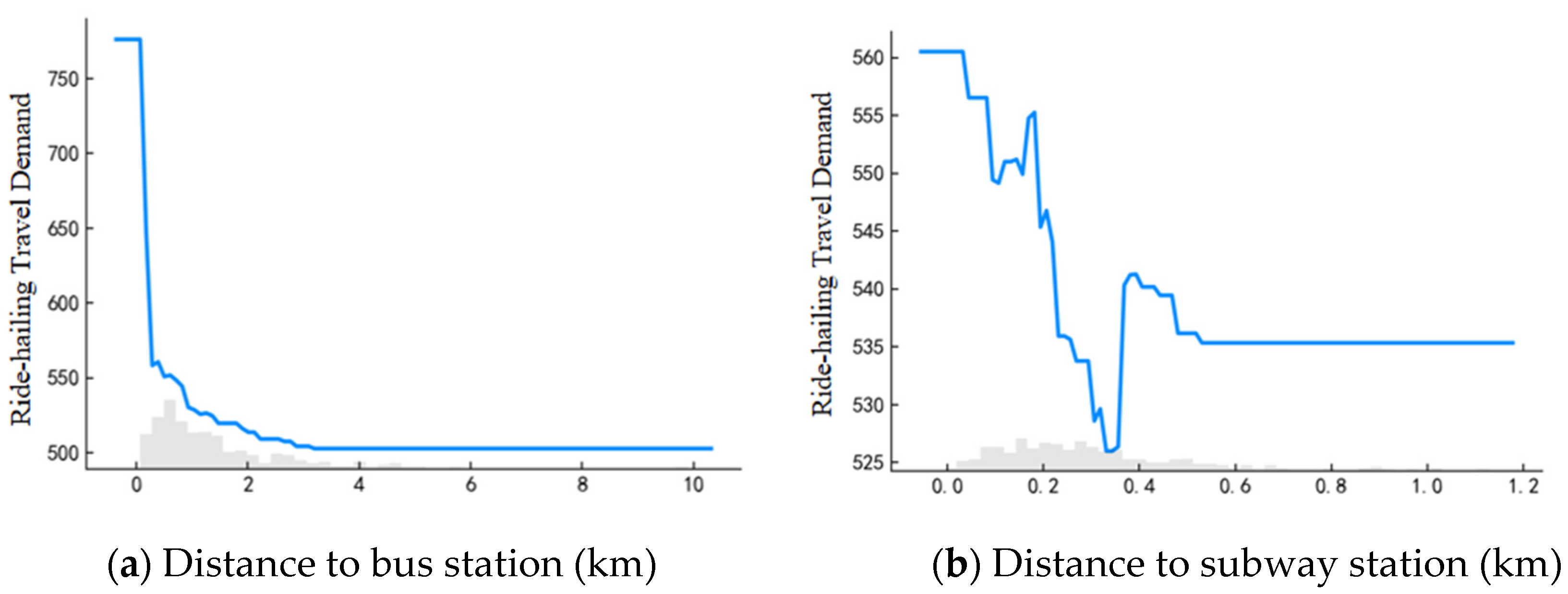
As shown in Figure 7a, When the distance to the bus station falls within the range of approximately 0 to 0.5 km, there is a significant decline in ride-hailing travel demand. Beyond a distance of 3 km, the impact of ride-hailing tends to stabilize. Similarly, as illustrated in Figure 7b, the distance to the metro station shows a continuous reduction in ride-hailing travel demand within the range of 0 to 0.35 km, reaching its lowest point at 0.35 km. This phenomenon may be attributed to the integration of ride-hailing with public transportation, aiming to address the “last-mile” problem of commuting [32,33]. We also observed that bus stations have a larger radius of influence. Conversely, the ride-hailing travel demand increases slightly after reaching a distance of 0.4 km from metro stations, and then stabilizes. This may be because ride-hailing services complement the “first-mile” commute to connect with metro stations, contributing to this phenomenon.
6. Conclusions
This study utilizes ride-hailing data from Nanjing and integrates multi-source data including population, urban road network, POI, and public transportation stations to characterize built environment indicators from the perspective of the “5Ds”. By applying the XGBoost model, the study explores the impact of built environment factors on ride-hailing travel demand. Through the combined analysis of SHAP and PDPs, the study elucidates the contribution, nonlinearity, and threshold impacts of built environment features on predicting ride-hailing travel demand. The research findings provide valuable insights for urban development, transportation planning, and ride-hailing resource allocation.
Firstly, the article estimated the average relative importance of the “5Ds” and assessed the relative importance and ranking of various built environment features on ride-hailing travel demand. The results indicate that the density dimension has the highest average relative importance at 7.89%, and the contribution rate of dining facilities to predicting ride-hailing travel demand is highest at 30.75%. Secondly, through the SHAP summary plot analysis, the article examined how built environment features positively or negatively affect the target variable. Based on the SHAP feature ranking, it was found that the top four built environment features are dining, finance, company, and medical facilities, all of which are POI facilities. TNCs should prioritize the supply and allocation of ride-hailing vehicles around these built environment features. Finally, through the PDPs plot visualization, the article illustrated the nonlinearity and threshold effects between built environment features and ride-hailing travel demand. The results indicate that built environment features need to reach a certain threshold or be within a certain range to exert the maximum impact on ride-hailing travel demand, with different thresholds and ranges for different built environment features. Analyzing the marginal impacts of population density, land use mix, and distance to subway stations revealed their comprehensive impact on ride-hailing travel demand. Understanding the nonlinearity and threshold effects between built environment variables and ride-hailing travel demand can help TNCs allocate ride-hailing resources reasonably and prevent overuse.
The article has certain limitations, and future research could explore the following aspects: (1) The study focused on ride-hailing travel demand over a typical workweek without analyzing specific periods. However, ride-hailing travel demand typically exhibits peak and off-peak periods during the day, and demand characteristics may vary from weekdays to weekends [38]. Clarifying the nonlinear impacts of factors influencing ride-hailing travel demand during different periods is important. Future research could investigate how factors such as built environment features influence ride-hailing travel demand during peak and off-peak hours, both on weekdays and weekends. (2) Due to the similarity of temporal and spatial features in the demand for ride-hailing services within a certain period, this study only utilizes weekly trip volumes for analysis [38,46]. In future research, we plan to employ more data to compare and analyze differences between weeks, thereby providing a more accurate reflection of the nonlinear threshold effects of the built environment on ride-hailing travel services. (3) Both built environment features and ride-hailing travel demand possess spatial attributes. Future research could analyze spatial effects in machine learning models. It could investigate whether interpretable machine learning models incorporating spatial effects outperform traditional geographically weighted models or exhibit similar or improved performance. This comparative examination would shed light on the effectiveness of different modeling approaches in capturing the spatial dynamics of ride-hailing travel demand affected by built environment features.
Author Contributions
Conceptualization, J.M., F.Z., W.T. and J.Y.; methodology, J.M. and W.T.; software, F.Z.; validation, J.Y. and F.Z.; writing—original draft preparation, J.Y. and F.Z.; writing—review and editing, J.M., F.Z., W.T. and J.Y.; visualization, F.Z. and J.Y.; supervision, J.M., W.T. and F.Z.; funding acquisition, F.Z. and J.Y. All authors have read and agreed to the published version of the manuscript.
Funding
This research was funded by the Postgraduate Research & Practice Innovation Program of Jiangsu Province, grant number SJCX23_0341.
Institutional Review Board Statement
Not applicable.
Informed Consent Statement
Not applicable.
Data Availability Statement
The data belongs to the Nanjing regulatory platform. The data are not publicly available due to privacy.
Acknowledgments
We would like to thank the data support provided by the Nanjing regulatory platform.
Conflicts of Interest
The authors declare no conflicts of interest.
References
- Rayle, L.; Dai, D.; Chan, N.; Cervero, R.; Shaheen, S. Just a better taxi? A survey-based comparison of taxis, transit, and ridesourcing services in San Francisco. Transp. Policy 2016, 45, 168–178. [Google Scholar] [CrossRef]
- Young, M.; Allen, J.; Farber, S. Measuring when Uber behaves as a substitute or supplement to transit: An examination of travel-time differences in Toronto. J. Transp. Geogr. 2020, 82, 102629. [Google Scholar] [CrossRef]
- Zhang, B.; Chen, S.; Ma, Y.; Li, T.; Tang, K. Analysis on spatiotemporal urban mobility based on online car-hailing data. J. Transp. Geogr. 2020, 82, 102568. [Google Scholar] [CrossRef]
- Shi, K.; Shao, R.; De Vos, J.; Cheng, L.; Witlox, F. The influence of ride-hailing on travel frequency and mode choice. Transp. Res. Part D Transp. Environ. 2021, 101, 103125. [Google Scholar] [CrossRef]
- Yin, C.; Lu, Y.; Shao, C.; Ma, J.; Xu, D. Impacts of built environment on commuting mode choice considering spatial autocorrelation. J. Jilin Univ. (Eng. Technol. Ed.) 2023, 53, 1994–2000. [Google Scholar] [CrossRef]
- Wang, X.; Shao, C.; Yin, C.; Guan, L. Exploring the relationships of the residential and workplace built environment with commuting mode choice: A hierarchical cross-classified structural equation model. Transp. Lett. 2022, 14, 274–281. [Google Scholar] [CrossRef]
- Yin, C.; Wang, X.; Shao, C.; Ma, J. Exploring the Relationship between Built Environment and Commuting Mode Choice: Longitudinal Evidence from China. Int. J. Environ. Res. Public Health 2022, 19, 14149. [Google Scholar] [CrossRef] [PubMed]
- Du, Q.; Zhou, Y.; Huang, Y.; Wang, Y.; Bai, L. Spatiotemporal exploration of the non-linear impacts of accessibility on metro ridership. J. Transp. Geogr. 2022, 102, 103380. [Google Scholar] [CrossRef]
- Peng, B.; Zhang, Y.; Li, C.; Wang, T.; Yuan, S. Nonlinear, threshold and synergistic effects of first/last-mile facilities on metro ridership. Transp. Res. Part D Transp. Environ. 2023, 121, 103856. [Google Scholar] [CrossRef]
- Chen, C.; Feng, T.; Ding, C.; Yu, B.; Yao, B. Examining the spatial-temporal relationship between urban built environment and taxi ridership: Results of a semi-parametric GWPR model. J. Transp. Geogr. 2021, 96, 103172. [Google Scholar] [CrossRef]
- Qian, X.; Ukkusuri, S.V. Spatial variation of the urban taxi ridership using GPS data. Appl. Geogr. 2015, 59, 31–42. [Google Scholar] [CrossRef]
- Zhu, P.; Li, J.; Wang, K.; Huang, J. Exploring spatial heterogeneity in the impact of built environment on taxi ridership using multiscale geographically weighted regression. Transportation 2023. [Google Scholar] [CrossRef]
- Ma, X.; Ji, Y.; Yuan, Y.; Van Oort, N.; Jin, Y.; Hoogendoorn, S. A comparison in travel patterns and determinants of user demand between docked and dockless bike-sharing systems using multi-sourced data. Transp. Res. Part A Policy Pract. 2020, 139, 148–173. [Google Scholar] [CrossRef]
- Wang, Y.; Li, J.; Su, D.; Zhou, H. Spatial-temporal heterogeneity and built environment nonlinearity in inconsiderate parking of dockless bike-sharing. Transp. Res. Part A: Policy Pract. 2023, 175, 103789. [Google Scholar] [CrossRef]
- Wang, X.; Shao, C.; Yin, C.; Dong, C. Exploring the effects of the built environment on commuting mode choice in neighborhoods near public transit stations: Evidence from China. Transp. Plan. Technol. 2021, 44, 111–127. [Google Scholar] [CrossRef]
- Wang, X.; Shao, C.; Yin, C.; Zhuge, C. Exploring the Influence of Built Environment on Car Ownership and Use with a Spatial Multilevel Model: A Case Study of Changchun, China. Int. J. Environ. Res. Public Health 2018, 15, 1868. [Google Scholar] [CrossRef] [PubMed]
- Yin, C.; Shao, C.; Wang, X. Exploring the impact of built environment on car use: Does living near urban rail transit matter? Transp. Lett. 2020, 12, 391–398. [Google Scholar] [CrossRef]
- Dean, M.D.; Kockelman, K.M. Spatial variation in shared ride-hail trip demand and factors contributing to sharing: Lessons from Chicago. J. Transp. Geogr. 2021, 91, 102944. [Google Scholar] [CrossRef]
- Fotheringham, A.S.; Charlton, M.E.; Brunsdon, C. Geographically Weighted Regression: A Natural Evolution of the Expansion Method for Spatial Data Analysis. Environ. Plan. A 1998, 30, 1905–1927. [Google Scholar] [CrossRef]
- Liu, F.; Gao, F.; Yang, L.; Han, C.; Hao, W.; Tang, J. Exploring the spatially heterogeneous effect of the built environment on ride-hailing travel demand: A geographically weighted quantile regression model. Travel Behav. Soc. 2022, 29, 22–33. [Google Scholar] [CrossRef]
- Wang, S.; Noland, R.B. Variation in ride-hailing trips in Chengdu, China. Transp. Res. Part D Transp. Environ. 2021, 90, 102596. [Google Scholar] [CrossRef]
- Yu, H.; Peng, Z.-R. Exploring the spatial variation of ridesourcing demand and its relationship to built environment and socioeconomic factors with the geographically weighted Poisson regression. J. Transp. Geogr. 2019, 75, 147–163. [Google Scholar] [CrossRef]
- Ji, S.; Wang, X.; Lyu, T.; Liu, X.; Wang, Y.; Heinen, E.; Sun, Z. Understanding cycling distance according to the prediction of the XGBoost and the interpretation of SHAP: A non-linear and interaction effect analysis. J. Transp. Geogr. 2022, 103, 103414. [Google Scholar] [CrossRef]
- Tao, T.; Cao, J. Exploring nonlinear and collective influences of regional and local built environment characteristics on travel distances by mode. J. Transp. Geogr. 2023, 109, 103599. [Google Scholar] [CrossRef]
- Tu, M.; Li, W.; Orfila, O.; Li, Y.; Gruyer, D. Exploring nonlinear effects of the built environment on ridesplitting: Evidence from Chengdu. Transp. Res. Part D Transp. Environ. 2021, 93, 102776. [Google Scholar] [CrossRef]
- Ghaffar, A.; Mitra, S.; Hyland, M. Modeling determinants of ridesourcing usage: A census tract-level analysis of Chicago. Transp. Res. Part C Emerg. Technol. 2020, 119, 102769. [Google Scholar] [CrossRef]
- Gomez, J.; Aguilera-García, Á.; Dias, F.F.; Bhat, C.R.; Vassallo, J.M. Adoption and frequency of use of ride-hailing services in a European city: The case of Madrid. Transp. Res. Part C Emerg. Technol. 2021, 131, 103359. [Google Scholar] [CrossRef]
- Dong, X. Trade Uber for the Bus? An Investigation of Individual Willingness to Use Ride-Hail Versus Transit. J. Am. Plan. Assoc. 2020, 86, 222–235. [Google Scholar] [CrossRef]
- Loa, P.; Habib, K.N. Examining the influence of attitudinal factors on the use of ride-hailing services in Toronto. Transp. Res. Part A Policy Pract. 2021, 146, 13–28. [Google Scholar] [CrossRef]
- Ewing, R.; Cervero, R. Travel and the Built Environment: A meta-analysis. J. Am. Plan. Assoc. 2010, 76, 265–294. [Google Scholar] [CrossRef]
- Ewing, R.; Cervero, R. Travel and the Built Environment: A Synthesis. Transp. Res. Rec. J. Transp. Res. Board 2001, 1780, 87–114. [Google Scholar] [CrossRef]
- Alemi, F.; Circella, G.; Handy, S.; Mokhtarian, P. What influences travelers to use Uber? Exploring the factors affecting the adoption of on-demand ride services in California. Travel Behav. Soc. 2018, 13, 88–104. [Google Scholar] [CrossRef]
- Sabouri, S.; Park, K.; Smith, A.; Tian, G.; Ewing, R. Exploring the influence of built environment on Uber demand. Transp. Res. Part D Transp. Environ. 2020, 81, 102296. [Google Scholar] [CrossRef]
- Wang, X.; Yin, C.; Zhang, J.; Shao, C.; Wang, S. Nonlinear effects of residential and workplace built environment on car dependence. J. Transp. Geogr. 2021, 96, 103207. [Google Scholar] [CrossRef]
- He, M.; Pu, L.; Liu, Y.; Shi, Z.; He, C.; Lei, J. Research on Nonlinear Associations and Interactions for Short-Distance Travel Mode Choice of Car Users. J. Adv. Transp. 2022, 2022, 8598320. [Google Scholar] [CrossRef]
- Jin, T.; Cheng, L.; Zhang, X.; Cao, J.; Qian, X.; Witlox, F. Nonlinear effects of the built environment on metro-integrated ridesourcing usage. Transp. Res. Part D Transp. Environ. 2022, 110, 103426. [Google Scholar] [CrossRef]
- Statistical Communiqué on National Economic and Social Development of Nanjing in 2022. Available online: https://tjj.nanjing.gov.cn/bmfw/njsj/202303/t20230324_3871176.html (accessed on 12 October 2023).
- He, Z. Portraying ride-hailing mobility using multi-day trip order data: A case study of Beijing, China. Transp. Res. Part A Policy Pract. 2021, 146, 152–169. [Google Scholar] [CrossRef]
- Li, X.; Xu, J.; Du, M.; Liu, D.; Kwan, M.-P. Understanding the spatiotemporal variation of ride-hailing orders under different travel distances. Travel Behav. Soc. 2023, 32, 100581. [Google Scholar] [CrossRef]
- Zhao, F.; Ma, J.; Yin, C.; Tang, W.; Wang, X.; Yin, J. Spatiotemporal Heterogeneous Effects of Built Environment and Taxi Demand on Ride-Hailing Ridership. Appl. Sci. 2024, 14, 142. [Google Scholar] [CrossRef]
- Chen, T.; Guestrin, C.; Assoc Comp, M. XGBoost: A Scalable Tree Boosting System. In Proceedings of the 22nd ACM SIGKDD International Conference on Knowledge Discovery and Data Mining (KDD), San Francisco, CA, USA, 13–17 August 2016; pp. 785–794. [Google Scholar] [CrossRef]
- Shapley, L.S. A Value for N-Person Games; RAND Corporation: Santa Monica, CA, USA, 1952. [Google Scholar] [CrossRef]
- Lundberg, S.; Lee, S.-I. A Unified Approach to Interpreting Model Predictions. In Proceedings of the 31st International Conference on Neural Information Processing Systems (NIPS’17), Long Beach, CA, USA, 4–9 December 2017; Volume 30, p. 07874. [Google Scholar]
- Štrumbelj, E.; Kononenko, I. Explaining prediction models and individual predictions with feature contributions. Knowl. Inf. Systs. 2014, 41, 647–665. [Google Scholar] [CrossRef]
- Li, Z. Extracting spatial effects from machine learning model using local interpretation method: An example of SHAP and XGBoost. Comput. Environ. Urban Syst. 2022, 96, 101845. [Google Scholar] [CrossRef]
- Lyu, T.; Wang, Y.; Ji, S.; Feng, T.; Wu, Z. A multiscale spatial analysis of taxi ridership. J. Transp. Geogr. 2023, 113, 103718. [Google Scholar] [CrossRef]
Figure 1.
Study area.
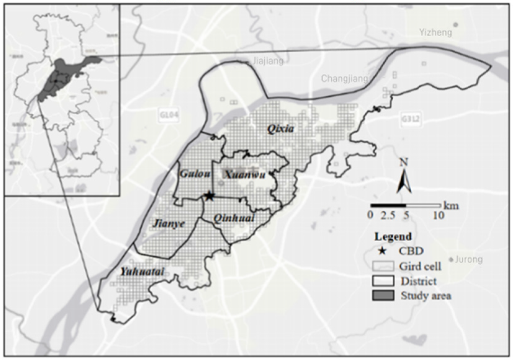
Figure 2.
SHAP summary plot of independent variables.

Figure 3.
Nonlinear effect of density variables on ride-hailing travel demand.
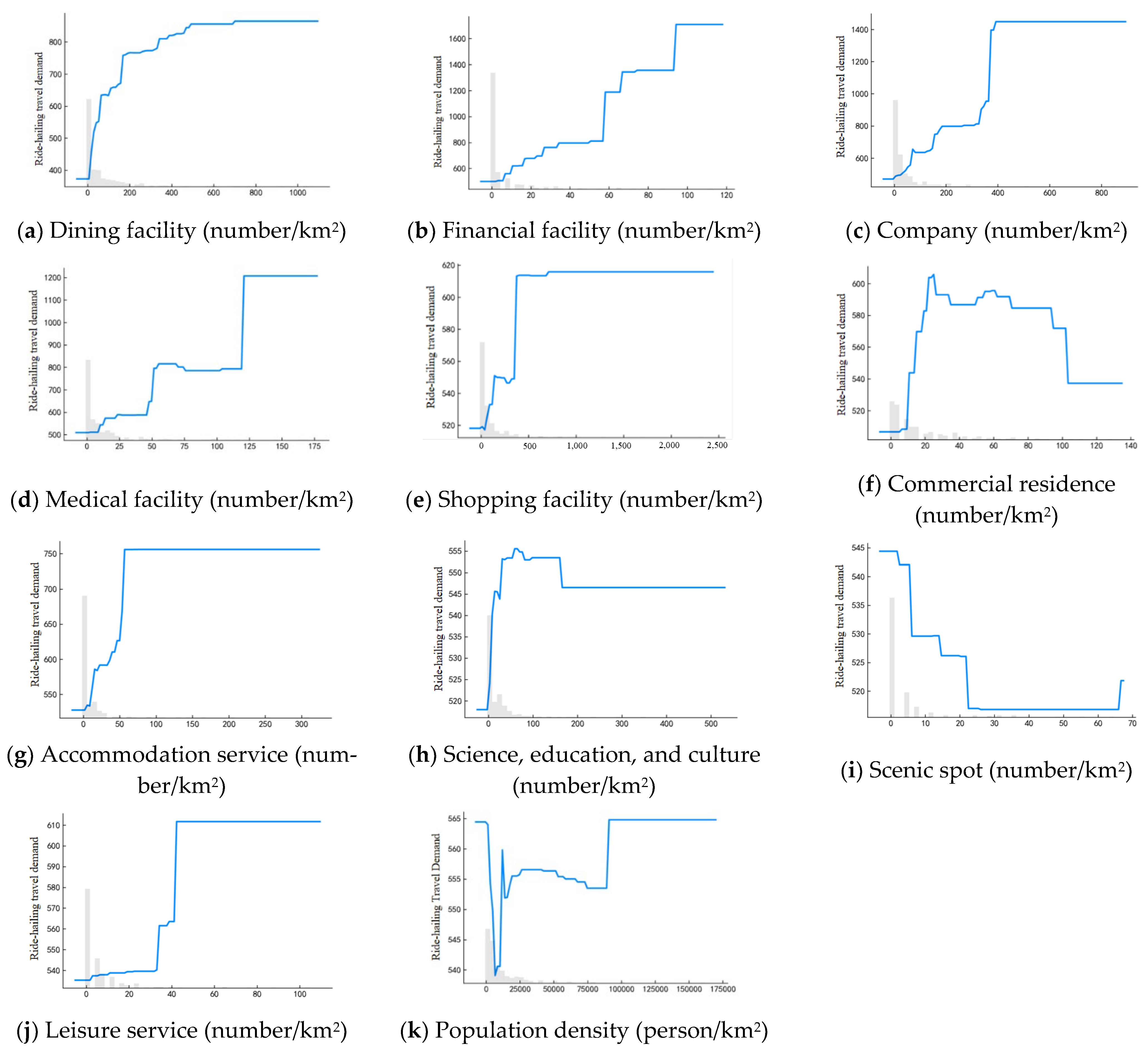
Figure 4.
Nonlinear effect of design variables on ride-hailing travel demand.
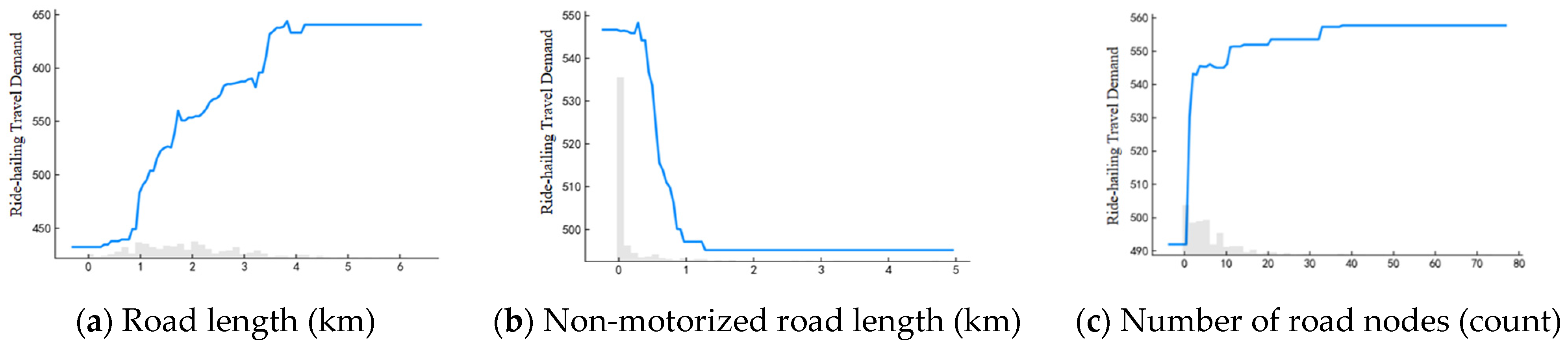
Figure 5.
Nonlinear effect of diversity variables on ride-hailing travel demand.
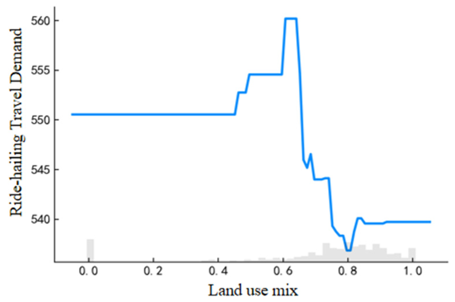
Figure 6.
Nonlinear effect of destination accessibility on ride-hailing travel demand.
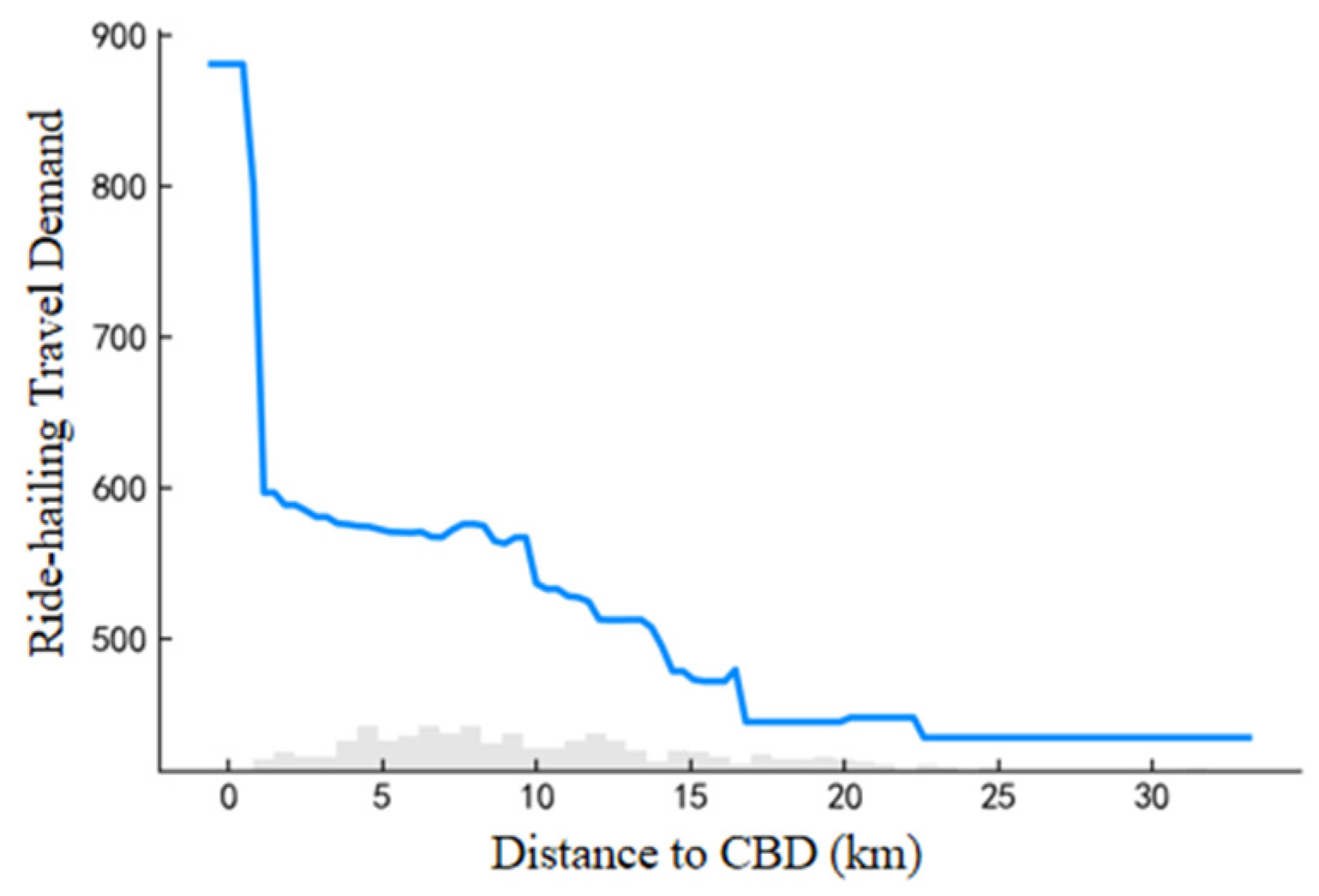
Figure 7.
Nonlinear effect of distance to transit on ride-hailing travel demand.

Table 1.
Examples of the ride-hailing orders in the dataset.
| Order ID | Vehicle ID | Pick-Up Time | Drop-Off Time | Pick-Up Location (LON, LAT) | Drop-Off Location (LON, LAT) |
|---|---|---|---|---|---|
| TS120220411012600XXX | SADXXX87 | 2022/4/11 01:33:59 | 2022/4/11 01:50:56 | (118.746650, 32.021847) | (118.787378, 32.048361) |
| 15fb8a0ea4422477fXXX | SA1XXXY | 2022/4/12 09:59:20 | 2022/4/12 10:21:39 | (118.823082, 31.964883) | (118.637144, 31.930987) |
| TS120220413155000XXX | SADXXX19 | 2022/4/13 15:54:21 | 2022/4/13 16:20:28 | (118.787103, 32.069792) | (118.734399, 32.127606) |
| TS120220414151003XXX | SADXXX53 | 2022/4/14 15:14:28 | 2022/4/14 15:33:21 | (118.816308, 32.066452) | (118.763203, 32.009617) |
| 17753565138XXX | SA8XXXC | 2022/4/15 12:34:17 | 2022/4/15 12:44:36 | (118.779821, 32.029380) | (118.787625, 32.043140) |
Table 2.
Descriptive statistics of variables.
| Variable | Description | Mean | S.D. | Source |
|---|---|---|---|---|
| Dependent variables | ||||
| Ride-hailing travel demand | Number of ride-hailing trips divided by the grid area (count/km2) | 536.22 | 712.48 | Nanjing Transport |
| Independent variables | ||||
| Density | ||||
| Population density | Population size divided by the grid area (person/km2) | 12,641.95 | 19,460.06 | WorldPop |
| Dining facility | Number of dining facilities divided by the grid area (count/km2) | 69.09 | 130.90 | Chinese Amap |
| Company | Number of companies divided by the grid area (count/km2) | 37.79 | 67.99 | Chinese Amap |
| Shopping facility | Number of shopping facilities divided by the grid area (count/km2) | 99.77 | 228.37 | Chinese Amap |
| Financial facility | Number of financial facilities divided by the grid area (count/km2) | 6.41 | 16.57 | Chinese Amap |
| Accommodation service | Number of accommodation services divided by the grid area (count/km2) | 11.26 | 32.99 | Chinese Amap |
| Science, education, and culture | Number of science, education, and culture facilities divided by the grid area (count/km2) | 22.99 | 44.82 | Chinese Amap |
| Scenic spot | Number of scenic spots divided by the grid area (count/km2) | 5.23 | 18.76 | Chinese Amap |
| Commercial residence | Number of commercial residences divided by the grid area (count/km2) | 17.79 | 24.02 | Chinese Amap |
| Leisure service | Number of leisure services divided by the grid area (count/km2) | 5.32 | 12.40 | Chinese Amap |
| Medical facility | Number of medical facilities divided by the grid area (count/km2) | 12.87 | 23.21 | Chinese Amap |
| Design | ||||
| Road length | The length of roads divided by the grid area (km/km2) | 1.97 | 1.15 | OpenStreetMap |
| Non-motorized road length | The length of non-motorized roads divided by the grid area (km/km2) | 0.21 | 0.51 | OpenStreetMap |
| Number of road nodes | Number of road nodes divided by the grid area (count/km2) | 7.07 | 9.31 | OpenStreetMap |
| Diversity | ||||
| Land use mix | The entropy value of thirteen categories of POI | 0.71 | 0.28 | Chinese Amap |
| Destination accessibility | ||||
| Distance to CBD | Distance from the grid centroid to CBD (km) | 10.16 | 5.73 | Chinese Amap |
| Distance to transit | ||||
| Distance to bus stop | Distance from the grid centroid to the nearest bus stop (km) | 0.31 | 0.21 | Chinese Amap |
Table 3.
The relative importance of independent variables.
| Variables | Relative Importance | Ranking |
|---|---|---|
| Density (average of relative importance: 7.89%) | ||
| Population density | 1.36% | 15 |
| Dining facility | 30.75% | 1 |
| Company | 5.94% | 4 |
| Shopping facility | 4.86% | 5 |
| Financial facility | 26.42% | 2 |
| Accommodation service | 3.19% | 7 |
| Science, education, and culture | 1.34% | 16 |
| Scenic spot | 0.59% | 18 |
| Commercial residence | 3.56% | 6 |
| Leisure service | 2.55% | 9 |
| Medical facility | 6.28% | 3 |
| Design (average of relative importance: 1.86%) | ||
| Road length | 2.07% | 10 |
| Non-motorized road length | 1.88% | 11 |
| Number of road nodes | 1.63% | 13 |
| Diversity (average of relative importance: 1.48%) | ||
| Land use mix | 1.48% | 14 |
| Destination accessibility (sum of relative importance: 3.05%) | ||
| Distance to CBD | 3.05% | 8 |
| Distance to transit (average of relative importance: 1.53%) | ||
| Distance to bus stop | 1.23% | 17 |
| Distance to subway station | 1.82% | 12 |
Disclaimer/Publisher’s Note: The statements, opinions and data contained in all publications are solely those of the individual author(s) and contributor(s) and not of MDPI and/or the editor(s). MDPI and/or the editor(s) disclaim responsibility for any injury to people or property resulting from any ideas, methods, instructions or products referred to in the content. |
© 2024 by the authors. Licensee MDPI, Basel, Switzerland. This article is an open access article distributed under the terms and conditions of the Creative Commons Attribution (CC BY) license (https://creativecommons.org/licenses/by/4.0/).
Share and Cite
MDPI and ACS Style
Yin, J.; Zhao, F.; Tang, W.; Ma, J. The Nonlinear and Threshold Effect of Built Environment on Ride-Hailing Travel Demand. Appl. Sci. 2024, 14, 4072. https://doi.org/10.3390/app14104072
AMA Style
Yin J, Zhao F, Tang W, Ma J. The Nonlinear and Threshold Effect of Built Environment on Ride-Hailing Travel Demand. Applied Sciences. 2024; 14(10):4072. https://doi.org/10.3390/app14104072
Chicago/Turabian StyleYin, Jiexiang, Feiyan Zhao, Wenyun Tang, and Jianxiao Ma. 2024. "The Nonlinear and Threshold Effect of Built Environment on Ride-Hailing Travel Demand" Applied Sciences 14, no. 10: 4072. https://doi.org/10.3390/app14104072
Note that from the first issue of 2016, this journal uses article numbers instead of page numbers. See further details here.