Abstract
Ensuring a consistently reliable power supply is paramount in power systems. Researchers are engaged in the pursuit of categorizing transmission line failures to design countermeasures for mitigating the associated financial losses. Our study employs a machine learning-based methodology, specifically the Conformer Convolution-Augmented Transformer model, to classify transmission line fault types. This model processes time series input data directly, eliminating the need for expert feature extraction. The training and validation datasets are generated through simulations conducted on a two-terminal transmission line, while testing is conducted on historical data consisting of 108 events that occurred in the Taiwan power system. Due to the limited availability of historical data, they are utilized solely for inference purposes. Our simulations are meticulously designed to encompass potential faults based on an analysis of historical data. A significant aspect of our investigation focuses on the impact of the sampling rate on input data, establishing that a rate of four samples per cycle is sufficient. This suggests that, for our specific classification tasks, relying on lower frequency data might be adequate, thereby challenging the conventional emphasis on high-frequency analysis. Eventually, our methodology achieves a validation accuracy of 100%, although the testing accuracy is lower at 88.88%. The discrepancy in testing accuracy can be attributed to the limited information and the small number of historical events, which pose challenges in bridging the gap between simulated data and real-world measurements. Furthermore, we benchmarked our method against the ELM model proposed in 2023, demonstrating significant improvements in testing accuracy.
1. Introduction
Transmission line protective relaying is crucial to maintaining reliable power system operation, involving three core functions: detection, classification, and fault localization []. These functions play a vital role in safeguarding the overall stability and integrity of the power grid, ensuring a continuous and uninterrupted supply of electricity. This study aims to enhance fault classification accuracy using machine learning (ML) techniques. Fault classification provides valuable information that significantly aids in quickly estimating fault locations, leading to faster fault-clearing times and the rapid restoration of power service []. In real-life scenarios, relays and circuit breakers are deployed to monitor the status of transmission lines. However, actuating the relay is time-consuming and this operation is more efficient using ML [].
ML-based techniques have garnered widespread acclaim in the domain of transmission line fault classification [,]. ML-based methods require substantial data to effectively train classifier models. While most studies rely on simulated data due to the scarcity of real-system fault data [,,,], our approach also incorporates historical event data from the Taiwan power system, comprising 108 events with varied fault scenarios. It is noteworthy that a laboratory physical system developed in [] generates a relevant dataset. These studies generate data through simulation considering different fault impedances, fault locations, fault inception angles (FIAs), circuit breaker time delays, transmission line configurations, source impedances, and the transposition of transmission lines [,,,,,,]. In this study, we train and validate our classifier model using simulated data but test it using historical event data collected from the Taiwan power system. The limited availability of historical data, particularly with some fault types represented by only a few cases, restricts our ability to use these data for training. Based on the analysis of the historical data, we generate various scenarios to emulate potential faults in the Taiwan power system more realistically.
The input data for the classifier model comprise measurements of three-phase voltage and currents obtained from either the single end or double end of a multi-terminal transmission line. However, most studies require preprocessing via feature extraction prior to training. Feature extraction is crucial in classification by isolating relevant and critical data from raw signals. For fault classification purposes, most feature extraction processes involve transforming the input time series data into the frequency domain. Previous research has introduced feature extraction methodologies such as wavelet packet transformation (WT) [,,,], multiwavelet packet transformation (MWT) [], Hilbert–Huang Transform (HHT) [], time series imaging [], and mathematical morphology (MM) []. The precise classification of faults in transmission lines through WTs necessitates dynamically adjusting their parameters according to the prevailing power system topology []. Additionally, selecting an appropriate mother wavelet for analysis is imperative to address specific fault scenarios. This strategic choice ensures optimal extraction of relevant features from the signal, facilitating the accurate identification and characterization of faults within the transmission line network. Although HHT in [] was used to eliminate the challenge of selecting a suitable mother wavelet for a WT, it is not applicable for wideband signals and requires high computational complexity. Though most studies focus on expert feature extraction, some studies apply time series raw data directly to their model [,]. Designing a model adept at directly processing raw time series data allows us to harness the power of machine learning to autonomously discern and delineate crucial patterns and characteristics, thereby enhancing the accuracy of fault classification. This approach not only streamlines the workflow but also elevates the model’s adaptability across diverse fault scenarios, ensuring its efficacy in real-world applications without the need of expert knowledge for feature extraction.
Applying the model to real-world data introduces numerous challenges, particularly concerning the diverse sampling rates of input data, where different types of relays each operate at specific sampling rates. In Taiwan, these rates range from 4 to 188.5 samples per cycle. In contrast, simulation-based studies typically utilize consistent sampling rates, such as 20 kHz (333.33 samples per cycle for 60 Hz or 400 samples per cycle for 50 Hz) [,,], 10 kHz (200 samples per cycle for 50 Hz) [,], 2.4 kHz (40 samples per cycle for 60 Hz) [], and 1000 Hz (20 samples per cycle for 50 Hz) []. It is crucial to recognize that a model trained at a specific sampling rate may not perform optimally when processing data at a different sampling rate. Our study highlights that the highest accuracy is achieved when the sampling rate during testing closely matches the training sampling rate, underscoring the importance of considering sampling variability in model training and validation. We explore two approaches to address the challenge of handling signals with varying sample rates. The first approach involves training the classifier model for several commonly used sample rates. However, this approach may not be suitable for scenarios where the model needs to handle sample rates significantly deviating from the range of the training sample rates. The second approach involves resampling the signal to align with the sample rate used during the training phase before feeding it into the neural network. Our research explores three models to handle different sampling rates: Model I adapts to various rates; Models II and III involve resampling the data to 16 and 4 samples per cycle, respectively. Notably, Model III, which simplifies input data to lower sampling rates, demonstrates that detailed high-frequency information may have minimal impact on fault classification. This finding suggests that for our specific classification tasks, focusing on lower frequency data could be sufficient, challenging the conventional emphasis on high-frequency analysis.
The existing literature has proposed a repertoire of machine learning models on transmission line fault classification, encompassing the Artificial Neural Network (ANN) [], Extreme Learning Model (ELM) [], Radial Basis Function (RBF) neural network [], Convolutional Neural Network (CNN) [,], Long Short-Term Memory (LSTM) [], self-attention CNN (SAT-CNN) [], Support Vector Machine (SVM) [,], and Decision Tree (DT) []. Furthermore, ensemble techniques have been extensively employed across various domains utilizing ML-based methodologies [,], and similarly, transmission line fault classification also utilizes these techniques []. In this study, our aim is to develop a model distinguished by its exceptional generalizability, thus significantly reducing the reliance on expert feature extraction. Therefore, our study utilizes the Conformer Convolution-Augmented Transformer model, known for integrating local and global information efficiently. The Conformer has the ability to outperform LSTM and other Recurrent Neural Networks (RNNs), which are two common models used for handling time-relevant input data, in terms of classification accuracy with the same set of parameters [], which is analogous to the three-phase voltage and current signals used in our study. In addition, the Conformer achieves higher accuracy in a similar training time compared to LSTM and other RNNs []. Notably, in Automatic Speech Recognition (ASR), the Conformer model has demonstrated its effectiveness by surpassing the performance of previous Transformer- and CNN-based models, achieving state-of-the-art accuracies [].
The main contributions of this study are listed below:
- Our ML-based model can classify time series inputs without the need for expert feature extraction.
- The window selection for fault classification must encompass pre-fault and fault states. Nonetheless, we have observed that some historical event data also include post-fault states. Consequently, our model is designed to successfully classify faults using data that either include or exclude post-fault states.
- Resampling the data using frequency domain information provides several advantages, including handling non-integer sampling rates, benefiting from batch normalization, and improving efficiency.
- Resampling the data to four samples per cycle is sufficient for fault classification, even if the resulting signal may not perfectly resemble a sine wave. This finding suggests that for our specific classification tasks, focusing on lower frequency data could be sufficient, challenging the conventional emphasis on high-frequency analysis.
- We conduct a comparative analysis between our method and the ELM described in [], which has been compared with 11 state-of-the-art approaches spanning from 2015 to 2022. Our method significantly outperformed the ELM, which achieved a testing accuracy of 62%, whereas our method recorded higher accuracies of 88.88%
The remaining sections of this paper are structured as follows: Section 2 introduces the proposed methodology, including the applied preprocessing techniques. Section 3 presents an overview of the historical event data and compares the performance of fault classification between our method and the ELM. Finally, Section 4 provides the conclusions drawn from the study.
2. Methodology
The presented work employs a machine learning-based approach to tackle the fault classification problem. The primary goal was to classify the fault type in transmission line faults, which involved 10 different labels: AG, BG, CG, AB, BC, CA, ABG, BCG, CAG, and ABC, where A, B, C, and G stand for phase A, phase B, phase C, and ground, respectively. These faults are classified as single line to ground faults (SLG), line to line faults (LL), double line to ground faults (2LG), and line to line to line faults (LLL). Only LLL faults are symmetrical, while the remaining faults are asymmetrical as shown in Figure 1. Classification is a fundamental task in machine learning aimed at assigning labels to data instances. For instance, given a dataset where each event is associated with a label, such as “AG” for event 1, the goal is to predict the correct label for each event. The accuracy of a classification model is typically assessed by comparing the predicted labels to the ground truth labels. For example, if a model accurately predicts the labels for 90 out of 100 events, the accuracy is computed as 90%. This evaluation metric reflects the proportion of correctly classified instances out of the total number of instances, providing a measure of the model’s performance in terms of label prediction accuracy.
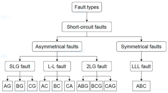
Figure 1.
Fault type classification.
The overview of the proposed method is illustrated in Figure 2. The input data for our classifier consist of three-phase voltage and current measurements from a single end of a two-terminal transmission line, resulting in six time series datasets. This approach differs from previous work that used data from both ends of the transmission line []. The data then undergo preprocessing, which includes window selection, resampling, and normalization. In this study, fault classification along the transmission line is performed using the Conformer model. The classifier outputs a predicted label, which in this case is the type of fault occurring on the transmission line.
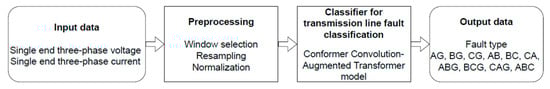
Figure 2.
Proposed fault classification scheme.
2.1. Data Generation for Training and Validation Datasets Using Simulation
ML-based approaches typically require substantial training data to achieve optimal performance. However, in scenarios where historical data may not provide sufficient diversity or uniformity in fault types, simulations can serve as a valuable tool to generate additional training and validation data []. In this study, we use Simulink simulations to create the training and validation datasets. The power system configuration used in the simulations is a two-terminal transmission line, as depicted in Figure 3. When the power flows from the ‘ABC’ to ‘abc,’ of a block, the power measurement is positive. Otherwise, the power measurement is negative. Consequently, the orientations of the blocks directly influence the resulting measurements. The system parameters of the simulations are listed in Table 1. The two-terminal transmission line configuration has been widely applied for the purpose of fault classification [,,,,,]. Based on the analysis of data from historical events, various fault scenarios were considered, encompassing different fault impedances, fault distances, circuit breaker time delays, FIAs, and fault types. We designed the fault impedance ranging from 0.1 to 10 Ohms, and the fault distance varied between 0.5 and 81 km, with a total transmission line length of 100 km. The circuit breaker time delay ranged from 2 cycles to infinity after the fault occurred, and the FIAs spanned from 0 to 315 degrees. By incorporating these factors into the simulations, we aim to create a comprehensive and diverse dataset that captures a wide range of potential fault scenarios in a transmission line. This comprehensive dataset allows us to evaluate and test the performance of our fault classification method across different fault conditions and parameters, providing a realistic and robust assessment of its effectiveness in handling various fault scenarios.
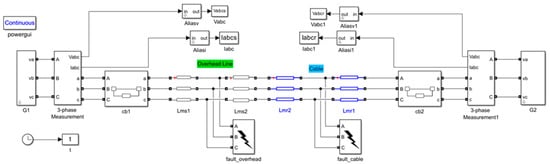
Figure 3.
Simulation model for a two-terminal transmission line using MATLAB Simulink.

Table 1.
Specification of the system parameters used for data generation.
To assess the model’s performance, a portion (15%) of the generated data was set aside as validation data, enabling the evaluation of the model’s classification accuracy on unseen instances. The validation results demonstrated that the model successfully classified both the training and testing data generated from simulations. This indicates that the model can effectively generalize and accurately classify fault types beyond the training set, providing confidence in its performance when applied to real-world scenarios using historical data for inference.
2.2. Preprocessing
In our approach, we avoid relying on expert experimentation in the preprocessing stage. Instead, we address three key topics related to the input data: window selection, normalization, and resampling. Each of these topics plays a crucial role in preparing the data for fault classification, and we will provide a brief overview of each.
Window selection: In fault events, there are typically three distinct states: pre-fault, fault, and post-fault, as illustrated in Figure 4. The post-fault state occurs after the fault has been cleared. In power systems, protective relays isolate the fault by opening circuit breakers once a fault is detected. As a result, the currents in Figure 4 decrease to zero after the fault is cleared. Our analysis shows that focusing exclusively on the pre-fault and fault states provides sufficient information to accurately categorize and identify faults in transmission lines. An adequately large window size that encompasses the relevant pre-fault and fault periods is crucial for capturing the necessary information for precise fault classification. Nonetheless, we have observed that some historical event data also include post-fault states. Consequently, our model is designed to successfully classify faults using data that either include or exclude post-fault states.
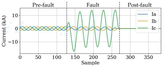
Figure 4.
Three-phase current waveform of a single line to ground fault (CG).
Normalization: Normalization is a vital technique to standardize the input data, ensuring a consistent range or distribution. By removing variations in signal magnitude or amplitude, this process enables the model to receive a uniform and comparable input across different samples. As a fundamental step in data preprocessing for machine learning applications, normalization is crucial for enhancing the model’s performance and accuracy. In this study, the normalization of phase voltage and current is carried out by dividing them by the root mean square value of the first cycle in the pre-fault state. The normalization process is illustrated in Figure 5.
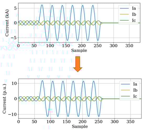
Figure 5.
Normalization of the three-phase current waveform.
Resampling: Resampling involves adjusting the sampling rate of input data to meet the specific requirements of the classifier model. This adjustment is crucial when the collected data have a different sampling rate than that required by the fault classification classifier model. Resampling ensures the input data’s consistency and compatibility with the model’s processing demands. However, most studies in the literature rely solely on simulation-generated data, which typically do not require resampling due to their consistent and pre-adjusted sampling rates. In this study, we apply the resampling method proposed in []. The process of resampling the signal using the Fast Fourier Transform (FFT) is illustrated as follows:
- Process the original signal using the Fast Fourier Transform (FFT) to obtain the signal spectrum in the frequency domain.
- Apply zero-padding or truncation to the spectrum to adjust it to the requested resampling rate. Zero-padding involves adding zeros to the spectrum to increase its length, while truncation involves removing unnecessary frequency components to reduce its length.
- After adjusting the spectrum, process the modified spectrum using the inverse Fast Fourier Transform (IFFT) to obtain the resampled signals in the time domain.
Following these steps, the signal is effectively resampled to the desired rate while preserving its essential information. This approach allows the model to handle signals with non-integer sampling rates, leading to more accurate fault classification and improved performance in transmission line fault classification applications. An example of data with a sampling rate of 188.5 samples per cycle, which have been resampled to 4 samples per cycle, is illustrated in Figure 6.
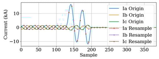
Figure 6.
Resampling from 188.5 to 4 samples per cycle of a single line to ground fault (AG).
Figure 7 provides examples of data that have been resampled to different sampling rates of 16 and 4 samples per cycle. The downsampling process from a higher to a lower sampling rate can introduce challenges in accurately representing the original signal, leading to potential distortions. With a lower sampling rate, the data may experience a loss of high-frequency information, resulting in a waveform that may not perfectly resemble a smooth sine wave. This distortion is evident in the resampled data with a sampling rate of 4 samples per cycle, as illustrated in Figure 7b. Such distortions can impact the accuracy of fault classification and introduce artifacts in the signal representation, potentially affecting the performance of the fault classification model. Furthermore, the phase issue becomes evident in the resampled data of 4 samples per cycle. Our approach addresses this problem by training the model with various inception angles, representing the phase angles at which the data are captured or sampled. By incorporating different inception angles during training, the model becomes more adept at handling diverse phase conditions, enhancing its robustness and generalization capabilities.
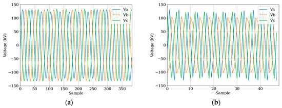
Figure 7.
Resampled voltage waveform. (a) Resample to 16 samples per cycle; (b) resample to 4 samples per cycle.
By addressing these preprocessing steps, including window selection, normalization, and resampling, the input data are appropriately prepared for subsequent analysis and fault classification tasks, leading to more accurate and reliable results.
2.3. Machine Learning-Based Model: Conformer: Convolution-Augmented Transformer Model
This study uses an ML-based method, employing the Conformer model []. The Conformer model is a state-of-the-art architecture commonly used in speech recognition tasks. It combines the Transformer model with the architecture of a CNN. The model architecture is illustrated in Figure 8.
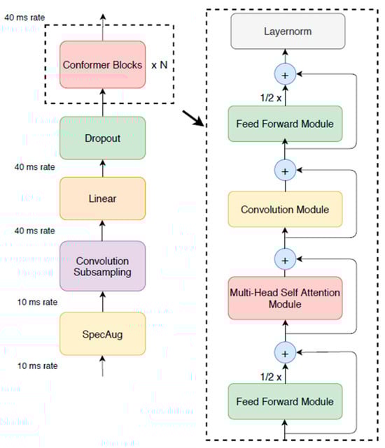
Figure 8.
Conformer encoder model architecture [].
A Conformer encoder model consists of four modules stacked together in sequence. These modules are as follows:
- Feed-forward module: This module processes the input data by applying a set of linear transformations and activation functions to capture relevant local features.
- Self-attention module []: The self-attention mechanism allows the Conformer to capture global dependencies and relationships within the input data.
- Convolution module: While the convolution module effectively captures local patterns, it requires many parameters and significant depth to capture global dependencies []. The parameters refer to the weights and bias in a neural network, while the depth refers to the number of layers in a neural network. To address this, batch normalization is applied immediately after the convolutional layers in deep neural networks. Batch normalization, a technique used in neural networks, normalizes each mini-batch of data during training. This normalization process transforms the data into a mean of 0 and a standard deviation of 1, following a standard normal distribution. This helps to alleviate the vanishing gradient problem and mitigate the effects of Internal Covariate Shift, which is the change in the distribution of the network’s internal activations during training. Additionally, batch normalization leverages the parallelism offered by modern computing platforms to significantly improve training efficiency []. To ensure the effective application of batch normalization, maintaining a uniform data length for each batch is essential. Resampling the data can help achieve this uniformity, ensuring that the input data have a consistent length, which is crucial for batch normalization to work optimally.
- Second feed-forward module: Similar to the first feed-forward module, this module further processes the output from the previous modules, refining and extracting additional features from the data.
By combining these four modules, the Conformer block effectively integrates local and global information, allowing it to model dependencies within the audio sequence in a parameter-efficient manner. The Conformer has the ability to outperform LSTM and other RNNs, which are common models used for handling time-relevant input data, in terms of classification accuracy with the same set of parameters []. This means that Conformer achieves higher accuracy in a similar training time compared to LSTM and other RNNs []. Furthermore, the Conformer model exhibits outstanding performance within a short training period by carefully designing the batch size in batch normalization.
Model hyper-parameters for Conformer are detailed in Table 2. The optimal Conformer model for fault classification purposes is determined by sweeping various combinations and selecting the best performing models within the parameter constraints. Our model, designed with 68,791 parameters and featuring three encoder layers with an encoder dimension of 128, requires significantly fewer parameters compared to the Conformer model for ASR purposes outlined in []. We observed that increasing the number of attention heads to three enhances accuracy, as each head focuses on different aspects of the input, thereby improving predictions beyond a simple weighted average. Furthermore, enlarging the convolution kernel size to five leads to better accuracy. Notably, we find that incorporating an LSTM decoder has little effect on the accuracy for fault classification, although it is commonly used in Conformer models for ASR purposes [].
Table 2.
Details of the model hyper-parameters for Conformer.
2.4. Methods Trained with Input Data at Various Sampling Rates
In this study, we implemented and compared three methods trained with input data at various sampling rates, as follows:
- Method I: The model is trained with data from various sampling rates [].
- Method II: The model is trained with data of 16 samples per cycle (960 Hz), and the input data are resampled to 16 samples per cycle.
- Method III: The model is trained with data of 4 samples per cycle (240 Hz), and the input data are resampled to 4 samples per cycle.
Table 3 summarizes the model parameter settings for the three methods employed in this study. The primary distinctions between the methods lie in the number of epochs and batch sizes utilized during training. Method I requires a higher number of epochs to achieve convergence, primarily due to its batch size of 1, which is necessary to maintain uniform data length for each batch. In contrast, Method II and Method III adopt a larger batch size of 128, as the input data are resampled to a consistent rate. This permits the utilization of larger batch sizes, which can improve training efficiency. This choice is further supported by evidence suggesting that using a small batch size may increase training time [], leading to longer training and inference times for Model I. Despite these variations in training setups, the classification results among the three methods are relatively similar, as will be demonstrated in the subsequent section.
Table 3.
Model parameter settings in each method.
Another technique to enhance the performance of the Transformer model is to use a warmup step and a learning rate scheduler []. The warmup step refers to the initial training phase where the learning rate is gradually increased from 0 until a predefined condition is met. Our project’s first 2 epochs of model training are dedicated to the warmup phase. Afterward, the learning rate follows a cosine function schedule for gradual reduction, as depicted in Figure 9.
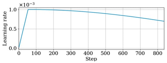
Figure 9.
Learning rate using warmup step and a learning rate scheduler.
2.5. Evaluation Metric
In our study, the model specifically targets single end data input. For a fault in a three-terminal transmission line, it produces three predicted fault types, one from each terminal. An event’s classification is considered accurate only if all terminals are accurately classified. If any terminal prediction is incorrect, the event prediction is marked as unsuccessful, denoted as pred = 0 in (1).
where is the number of terminals, is the predicted fault type for terminal i, and is the actual fault type of the event.
Subsequently, accuracy for the study is defined as the percentage of correctly predicted events among all events, calculated as (2):
where is the total number of events, and is the prediction for event j.
3. Simulation Results and Discussion
This study utilizes training and validation datasets generated from simulations, while the testing dataset is sourced from historical events. The classifier model is trained with the training dataset, which includes both features and labels. The validation and testing datasets are then used for inference. Classification accuracy is determined by comparing the predicted labels from the model with the actual labels in these datasets. Table 4 presents an overview of the training, validation, and testing datasets, with 85% of the data for training and 15% for validation.
Table 4.
Summary of training, validation, and testing datasets.
3.1. Summary of Historical Event Data
A total of 108 events are considered, encompassing various fault types such as single line to ground faults (SLG), line to line faults (LL), double line to ground faults (2LG), line to line to line faults (LLL), and line to line to line to ground faults (LLLG). These are detailed in Table 5. Historical events are utilized as testing data due to the limited occurrence of each fault type, suggesting that employing historical data for training purposes is feasible only with access to a more extensive dataset.
Table 5.
Fault types of historical events.
An analysis of these events led to the generation of datasets that encompass a broader range of scenarios, with characteristics summarized in Table 6. The historical events include various transmission line configurations: 25 events from two-terminal lines, 76 from three-terminal lines, and 7 from four-terminal lines. However, our findings indicate that training with data from three-terminal or four-terminal transmission lines does not significantly affect testing accuracy. Consequently, we chose to generate simulation data only for two-terminal transmission lines for efficiency. In the historical data collected, fault impedance values are unavailable, whereas fault distances, FIAs, and circuit breaker time delays are recorded. In Table 6, fault distances are presented in per unit (p.u.) terms with reference to the transmission line length: a fault at the left end is labeled as 0 p.u., and at the right end as 1 p.u. Our training and validation datasets are specifically designed to emulate the potential faults within the Taiwan power system, ensuring that they cover the range of fault distances, FIAs, and time delays observed in the historical events.
Table 6.
Summary of event characteristics in datasets.
In Taiwan, commonly used relay brands include SEL, Toshiba, GE, and Ingeteam. It is worth noting that the sampling rates for these relays can vary, ranging from 4 to 144 samples per cycle. As shown in Table 7, the largest number of events corresponds to a sampling rate of 16 samples per cycle.
Table 7.
Sampling rates of commonly used relay brands in Taiwan power system.
Data augmentation and transfer learning are powerful techniques for managing limited datasets in machine learning classification tasks. However, these methods must be carefully applied, as they can potentially amplify outliers or perpetuate biases present in the original data, especially when significant discrepancies exist between the simulated training data and real-world scenarios. Limited information on the events and the small number of available events have posed challenges in bridging the gap between simulated data and real-world measurements from the power system.
3.2. Issue of Multiple Input Sampling Rate
As indicated in Table 8, the accuracy of Model III decreases when it is tested with data sampled at different rates, particularly for data with sampling rates that differ significantly from the training sampling rate. The lowest validation accuracy, observed at a data sampling rate of 188.5 samples per cycle, is 47.37%. This indicates that the model’s performance is adversely affected when dealing with data at extreme sampling rates not encountered during its training phase. The impact of the sampling rate should be carefully considered when deploying the model in real-world scenarios. Matching or closely aligning the input data with the training sampling rate is crucial to preserve the accuracy and reliability of the model’s fault classification capabilities.
Table 8.
Results of data without resampling.
3.3. Comparison of Methods I, II, and III
Table 9 presents a comprehensive overview of the results obtained from Methods I, II, and III. Notably, the validation accuracies of these methods exhibit minimal variance. However, it is evident that Method III outperforms the other two approaches, with Method I yielding the lowest accuracy. As elucidated in Section 2, Method I requires a longer training time. Hence, for this study, Methods II and III emerge as more promising options. Both methods demonstrate competitive performance while offering potential time efficiency advantages compared to Method I. The testing accuracy exhibits a noticeable decrease compared to the training and validation accuracy across all methodologies. This disparity may be attributed to the omission of certain nonideal aspects present in the actual power system, which are not explicitly modeled in the simulations. Nonetheless, due to the constraints of limited historical data, relying on such data as the sole source for model training may not be advisable. To enhance the model’s performance, there arises a need for a more comprehensive dataset or the incorporation of supplementary measurements beyond voltage and current.
Table 9.
Results of Methods I, II, and III.
In this study, we investigate the performance of two models trained with different sampling rates: 16 samples per cycle (Model II) and 4 samples per cycle (Model III). The classification results of Methods II and III are presented in Table 10 and Table 11, respectively. Notably, Method II achieves the highest validation accuracy for 16 samples per cycle. In comparison, Method III performs best at a sampling rate of 4 samples per cycle. Interestingly, despite the differences in requested sampling rates, the results do not show significant discrepancies between these models. This suggests that training the models with a sampling rate of four samples per cycle is sufficient for the fault type classification task. Consequently, Method III, which utilizes the lower sampling rate, emerges as a more promising choice. Additionally, it shows that detailed high-frequency information may have minimal impact on fault classification. This approach offers the advantage of reduced computation in both the inference and training processes while still achieving comparable performance in fault type classification.
Table 10.
Validation and testing accuracy of Method II across various sampling rates.
Table 11.
Validation and testing accuracy of Method III across various sampling rates.
The testing accuracy of Methods II and III for various transmission line configurations is presented in Table 12. The testing accuracy for three- or four-terminal transmission lines remains notably low, regardless of whether the analysis includes all recorded events or only data from individual ends. Despite experimenting with various configurations, no improvement in validation or testing accuracy is observed. This suggests that our current consideration of different transmission impedances, fault distances, and fault inception angles may not adequately capture the complexities of potential faults in transmission lines. A thorough gap analysis is essential to identify factors or conditions present in real-world data that are absent in our simulations. Therefore, we need more comprehensive historical data to better simulate real-world fault conditions. Moreover, iteratively refining the model and simulation parameters based on real-world data feedback can progressively diminish the discrepancy between simulated and actual conditions. Overall, the low testing accuracy underscores the critical need for more comprehensive historical data to better mimic real-world fault conditions and to fully leverage the capabilities of big data for enhanced model performance.
Table 12.
Testing accuracy of Methods II and III across various transmission line configurations.
3.4. Comparison with the State-of-the-Art Method
We compare our methods (Methods II and III) with a previously developed approach using the ELM, described in [], which itself was compared with 11 state-of-the-art methods spanning from 2015 to 2022. In [], two different ELM models were developed for fault detection (binary labels) and fault classification (multi-labels) purposes, both featuring a hidden layer of 700 nodes. When a fault is detected using the ELM for fault detection, it is subsequently classified using the ELM for fault classification. The ELM is a type of artificial neural network (ANN) with one or more hidden layers. ELMs are known for their simple structure, no parameter adaptation, shorter processing times, and lower computational complexity.
Table 13 presents a performance comparison of Method II, Method III, and the ELM, all trained on the same training dataset. While training and validation accuracies are near 100% for all methods, testing accuracies vary significantly: the ELM achieves 62%, whereas Methods II and III record higher accuracies of 87.04% and 88.88%, respectively, demonstrating the superior performance of our models. In terms of prediction time on the validation dataset, the ELM requires the least time, followed by Method III, which is faster than Method II, likely due to the lower sampling rates utilized in Method III. Notably, the performance of the Conformer model is not significantly affected by changes in sampling rates. These inferences were conducted on a desktop PC equipped with Windows 11 Enterprise 22H2, and an NVIDIA GeForce RTX 3060 GPU sourced from Santa Clara, California, USA.
Table 13.
Comparison between our proposed method and state-of-the-art model.
Figure 10 illustrates the confusion matrixes on validation and testing datasets for the ELM, and Figure 11 for Method III. For the validation dataset, our methods accurately classify fault types across all terminals in all events, whereas the ELM has one instance of incorrect classification. Specifically, Figure 10a shows one CAG fault misclassified as CA. Figure 11b highlights the most significant misclassifications for Method III, with eleven AG faults misclassified as ABG, ten AG faults as CAG, and six BG faults as ABG. In contrast, Figure 10b shows four ABC faults misclassified as CAG, and two AG faults as CAG.
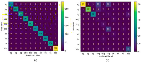
Figure 10.
Confusion matrix for ELM. (a) Validation dataset. (b) Testing dataset.
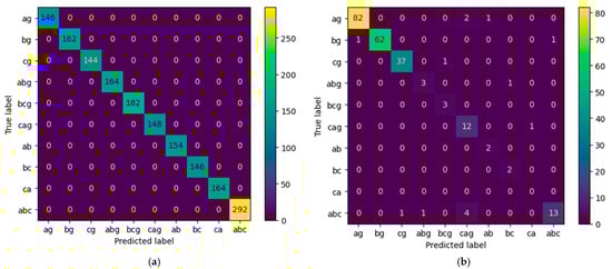
Figure 11.
Confusion matrix for Method III. (a) Validation dataset. (b) Testing dataset.
Table 14 details the testing accuracy of each fault type. For Method III, “ABG” and “ABC” fault types have notably low accuracies of 75.00% and 68.42%, respectively. For the ELM, fault types “AG”, “ABG”, “BC”, and “ABC” all have testing accuracies below 80%. Both models experience difficulties particularly with “ABG” and “ABC” fault types. To enhance performance, more comprehensive historical data are required to better simulate real-world fault conditions within the training dataset.
Table 14.
Performance of each fault type for Method III and ELM.
4. Conclusions
This study employs a machine learning-based method to classify transmission line faults using three-phase voltage and current measurements, utilizing a Conformer model. The goal of this research is to develop a model that generalizes effectively without relying on extensive expert-driven feature extraction. Traditionally, feature extraction plays a crucial role in fault classification by isolating relevant and critical data from raw signals. However, the Conformer Convolution-Augmented Transformer model used in this study demonstrates a remarkable ability to autonomously identify key features. This capability significantly reduces the need for predefined feature extraction. Our classifier is trained on simulation data from a two-terminal transmission line and tested on historical data from the Taiwan power system. It is important to note that, typically, studies in the literature rely solely on simulation data.
We collected 108 historical events across 10 fault types, which is generally insufficient for machine learning training purposes. Based on the analysis of these events, our training dataset is designed to cover various scenarios, including different fault types, fault impedances, fault distances, fault inception angle, and circuit breaker time delay.
Key preprocessing techniques explored include window selection, normalization, and resampling rate. Our findings indicate that including pre-fault and fault states in the window selection is crucial, whereas the inclusion of the post-fault state has a minimal impact on the model’s performance. Normalization involves dividing the measurements by the root mean square value of the first cycle in the pre-fault state. Although resampling is often overlooked in the literature, it is vital for data from the Taiwan power system where relay sampling rates vary from 4 to 188.5 samples per cycle. Resampling in the frequency domain effectively handles non-integer sampling rates, benefits from batch normalization, and enhances training efficiency. Our results show that resampling to 4 samples per cycle is adequate for fault classification, maintaining accuracy and reducing computational demands. This finding suggests that for our specific classification tasks, focusing on lower frequency data could be sufficient, challenging the conventional emphasis on high-frequency analysis.
Despite achieving a validation accuracy of 100%, the testing accuracy is lower at 88.88%, likely due to factors unaccounted for in the training dataset. This discrepancy underscores the need for more comprehensive historical data to better simulate real-world fault conditions and leverage the power of big data to enhance model performance. Moreover, we compared our method with the ELM proposed in 2023, and our method significantly outperformed the ELM in terms of testing accuracy.
Author Contributions
M.-Y.L., Y.-S.H., C.-W.L., T.-C.L. and Y.-B.L. designed the study. Y.-S.H., C.-J.C. and J.-Y.Y. performed transmission line fault simulations. M.-Y.L., Y.-S.H. and C.-J.C. analyzed the data. M.-Y.L. and Y.-S.H. wrote the paper with input from all authors. All authors have read and agreed to the published version of the manuscript.
Funding
This research was funded by National Atomic Research Institute grant number 112A019.
Institutional Review Board Statement
Not applicable.
Informed Consent Statement
Not applicable.
Data Availability Statement
The data are not publicly available due to the power company’s ownership. The testing datasets presented in this article are not readily available because they are the property of the Taipower company. Requests to access the datasets should be directed to the Taipower company.
Conflicts of Interest
The authors declare no conflicts of interest.
References
- Rahmati, A.; Adhami, R. A fault detection and classification technique based on sequential components. IEEE Trans. Ind. Appl. 2014, 50, 4202–4209. [Google Scholar] [CrossRef]
- Chen, K.; Huang, C.; He, J. Fault detection, classification and location for transmission lines and distribution systems: A review on the methods. High Volt. 2016, 1, 25–33. [Google Scholar] [CrossRef]
- Goni, M.O.F.; Nahiduzzaman, M.; Anower, M.S.; Rahman, M.M.; Islam, M.R.; Ahsan, M.; Haider, J.; Shahjalal, M. Fast and accurate fault detection and classification in transmission lines using extreme learning machine. e-Prime-Adv. Electr. Eng. Electron. Energy 2023, 3, 100107. [Google Scholar] [CrossRef]
- Nandhini, K.; Prajith, C. Review on Fault Detection and Classification in Transmission Line using Machine Learning Methods. In Proceedings of the 2023 International Conference on Control, Communication and Computing (ICCC), Thiruvananthapuram, India, 19–21 May 2023; pp. 1–6. [Google Scholar]
- Fang, J.; Chen, K.; Liu, C.; He, J. An Explainable and Robust Method for Fault Classification and Location on Transmission Lines. IEEE Trans. Ind. Inform. 2023, 19, 10182–10191. [Google Scholar] [CrossRef]
- Kanwal, S.; Jiriwibhakorn, S. Advanced Fault Detection, Classification, and Localization in Transmission Lines: A Comparative Study of ANFIS, Neural Networks, and Hybrid Methods. IEEE Access 2024, 12, 49017–49033. [Google Scholar] [CrossRef]
- Xi, Y.; Li, M.; Zhou, F.; Tang, X.; Li, Z.; Tian, J. SE-Inception-ResNet Model with Focal Loss for Transmission Line Fault Classification Under Class Imbalance. IEEE Trans. Instrum. Meas. 2023, 73, 3500917. [Google Scholar] [CrossRef]
- Guo, M.-F.; Yang, N.-C.; Chen, W.-F. Deep-learning-based fault classification using Hilbert–Huang transform and convolutional neural network in power distribution systems. IEEE Sens. J. 2019, 19, 6905–6913. [Google Scholar] [CrossRef]
- Godse, R.; Bhat, S. Mathematical morphology-based feature-extraction technique for detection and classification of faults on power transmission line. IEEE Access 2020, 8, 38459–38471. [Google Scholar] [CrossRef]
- Fahim, S.R.; Sarker, Y.; Sarker, S.K.; Sheikh, M.R.I.; Das, S.K. Self attention convolutional neural network with time series imaging based feature extraction for transmission line fault detection and classification. Electr. Power Syst. Res. 2020, 187, 106437. [Google Scholar] [CrossRef]
- Belagoune, S.; Bali, N.; Bakdi, A.; Baadji, B.; Atif, K. Deep learning through LSTM classification and regression for transmission line fault detection, diagnosis and location in large-scale multi-machine power systems. Measurement 2021, 177, 109330. [Google Scholar] [CrossRef]
- Jamil, M.; Sharma, S.K.; Singh, R. Fault detection and classification in electrical power transmission system using artificial neural network. SpringerPlus 2015, 4, 334. [Google Scholar] [CrossRef] [PubMed]
- Liu, Z.; Han, Z.; Zhang, Y.; Zhang, Q. Multiwavelet packet entropy and its application in transmission line fault recognition and classification. IEEE Trans. Neural Netw. Learn. Syst. 2014, 25, 2043–2052. [Google Scholar] [CrossRef]
- Moloi, K.; Ntombela, M.; Mosetlhe, T.C.; Ayodele, T.R.; Yusuff, A.A. Feature extraction based technique for fault classification in power distribution system. In Proceedings of the 2021 IEEE PES/IAS PowerAfrica, Virtual, 23–27 August 2021; pp. 1–5. [Google Scholar]
- Bon, N.N. Fault Identification, Classification, and Location on Transmission Lines Using Combined Machine Learning Methods. Int. J. Eng. Technol. Innov. 2022, 12, 91–109. [Google Scholar] [CrossRef]
- Kumar, P.; Bag, B.; Londhe, N.D.; Tikariha, A. Classification and Analysis of Power System Faults in IEEE-14 Bus System using Machine learning Algorithm. In Proceedings of the 2021 4th International Conference on Recent Developments in Control, Automation & Power Engineering (RDCAPE), Noida, India, 7–8 October 2021; pp. 122–126. [Google Scholar]
- Nusrat Jahan, P.; Anik, T.; Md, K.; Md Shanon, M.; Khadiza Tul, K. Short-Term Rainfall Prediction Using Supervised Machine Learning. Adv. Technol. Innov. 2023, 8, 111–120. [Google Scholar] [CrossRef]
- Tsehay Admassu, A.; Yenework Belayneh, C. The Performance of Machine Learning for Chronic Kidney Disease Diagnosis. Emerg. Sci. Innov. 2023, 1, 33–40. [Google Scholar] [CrossRef]
- Mishra, P.K.; Yadav, A.; Pazoki, M. A novel fault classification scheme for series capacitor compensated transmission line based on bagged tree ensemble classifier. IEEE Access 2018, 6, 27373–27382. [Google Scholar] [CrossRef]
- Shim, K.; Sung, W. A Comparison of Transformer, Convolutional, and Recurrent Neural Networks on Phoneme Recognition. arXiv 2022, arXiv:2210.00367. [Google Scholar]
- Gulati, A.; Qin, J.; Chiu, C.-C.; Parmar, N.; Zhang, Y.; Yu, J.; Han, W.; Wang, S.; Zhang, Z.; Wu, Y. Conformer: Convolution-augmented transformer for speech recognition. arXiv 2020, arXiv:2005.08100. [Google Scholar]
- Ferreira, V.; Zanghi, R.; Fortes, M.; Sotelo, G.; Silva, R.d.B.M.; Souza, J.; Guimarães, C.; Gomes Jr, S. A survey on intelligent system application to fault diagnosis in electric power system transmission lines. Electr. Power Syst. Res. 2016, 136, 135–153. [Google Scholar] [CrossRef]
- Virtanen, P.; Gommers, R.; Oliphant, T.E.; Haberland, M.; Reddy, T.; Cournapeau, D.; Burovski, E.; Peterson, P.; Weckesser, W.; Bright, J. SciPy 1.0: Fundamental algorithms for scientific computing in Python. Nat. Methods 2020, 17, 261–272. [Google Scholar] [CrossRef]
- Vaswani, A.; Shazeer, N.; Parmar, N.; Uszkoreit, J.; Jones, L.; Gomez, A.N.; Kaiser, Ł.; Polosukhin, I. Attention is all you need. Adv. Neural Inf. Process. Syst. arXiv 2017, arXiv:1706.03762. [Google Scholar]
- Bello, I.; Zoph, B.; Vaswani, A.; Shlens, J.; Le, Q.V. Attention augmented convolutional networks. In Proceedings of the IEEE/CVF International Conference on Computer Vision, Seoul, Republic of Korea, 27 October–2 November 2019; pp. 3286–3295. [Google Scholar]
- Ioffe, S.; Szegedy, C. Batch normalization: Accelerating deep network training by reducing internal covariate shift. In Proceedings of the International Conference on Machine Learning, Lille, France, 7–9 July 2015; pp. 448–456. [Google Scholar]
- Chowdhury, J. Sample-Rate Agnostic Recurrent Neural Network. Available online: https://jatinchowdhury18.medium.com/sample-rate-agnostic-recurrent-neural-networks-238731446b2 (accessed on 11 January 2024).
- Goyal, P.; Dollár, P.; Girshick, R.; Noordhuis, P.; Wesolowski, L.; Kyrola, A.; Tulloch, A.; Jia, Y.; He, K. Accurate, large minibatch sgd: Training imagenet in 1 hour. arXiv 2017, arXiv:1706.02677. [Google Scholar]
- Popel, M.; Bojar, O. Training tips for the transformer model. arXiv 2018, arXiv:1804.00247. [Google Scholar] [CrossRef]
Disclaimer/Publisher’s Note: The statements, opinions and data contained in all publications are solely those of the individual author(s) and contributor(s) and not of MDPI and/or the editor(s). MDPI and/or the editor(s) disclaim responsibility for any injury to people or property resulting from any ideas, methods, instructions or products referred to in the content. |
© 2024 by the authors. Licensee MDPI, Basel, Switzerland. This article is an open access article distributed under the terms and conditions of the Creative Commons Attribution (CC BY) license (https://creativecommons.org/licenses/by/4.0/).