
A Triple Deep Image Prior Model for Image Denoising Based on Mixed Priors and Noise Learning

School of Mathematics and Computer Sciences, Nanchang University, Nanchang 330031, China
*
Author to whom correspondence should be addressed.
Appl. Sci. 2023, 13(9), 5265; https://doi.org/10.3390/app13095265
Submission received: 1 April 2023
/
Revised: 16 April 2023
/
Accepted: 18 April 2023
/
Published: 23 April 2023
(This article belongs to the Section Computing and Artificial Intelligence)
Abstract
:Image denoising poses a significant challenge in computer vision due to the high-level visual task’s dependency on image quality. Several advanced denoising models have been proposed in recent decades. Recently, deep image prior (DIP), using a particular network structure and a noisy image to achieve denoising, has provided a novel image denoising method. However, the denoising performance of the DIP model still lags behind that of mainstream denoising models. To improve the performance of the DIP denoising model, we propose a TripleDIP model with internal and external mixed images priors for image denoising. The TripleDIP comprises of three branches: one for content learning and two for independent noise learning. We firstly use a Transformer-based supervised model (i.e., Restormer) to obtain a pre-denoised image (used as external prior) from a given noisy image, and then take the noisy image and the pre-denoised image as the first and second target image, respectively, to perform the denoising process under the designed loss function. We add constraints between two-branch noise learning and content learning, allowing the TripleDIP to employ external prior while enhancing independent noise learning stability. Moreover, the automatic stop criterion we proposed prevents the model from overfitting the noisy image and improves the execution efficiency. The experimental results demonstrate that TripleDIP outperforms the original DIP by an average of 2.79 dB and outperforms classical unsupervised methods such as N2V by an average of 2.68 dB and the latest supervised models such as SwinIR and Restormer by an average of 0.63 dB and 0.59 dB on the Set12 dataset. This can mainly be attributed to the fact that two-branch noise learning can obtain more stable noise while constraining the content learning branch’s optimization process. Our proposed TripleDIP significantly enhances DIP denoising performance and has broad application potential in scenarios with insufficient training datasets.
1. Introduction
The number of digital images has increased significantly with the popularization of imaging devices. Because image quality is often degraded by noise in the process of acquisition or transmission, image-denoising technology, which aims to extract noise while preserving image detail [1], has been used in various high-level visual tasks such as object detection [2], image generation [3], and semantic segmentation [4]. In most studies [5,6,7,8,9], degradation by noise is modeled by additive Gaussian white noise (AGWN) [10]. Its expression is:
where y represents the corrupted image, x denotes the undistorted image, and n denotes an additive noise that obeys a Gaussian distribution. Previously, various denoising algorithms [11,12,13,14,15,16] with different performance have been proposed, and they can be divided into three categories: filtering-based, model-based, and learning-based.
The non-local means (NLM) [17], block-matching3D (BM3D) [18] and weighted nuclear norm minimization (WNNM) [19] represent the standard filter-based denoising algorithms, which utilize the intrinsic statistics of the image patch for denoising. Typically, model-based methods define the task of denoising as an optimization problem using the maximum a posteriori (MAP) approach including nonlocally centralized sparse representation (NCSR) [20] and multivariate sparse regularization (MUSR) [21]. Although these methods can significantly decrease the image’s noise, they have to encounter the problem of computational efficiency, over-smoothness, and parameter selection. Compared with conventional methods, the learn-based approaches can achieve more satisfactory noise fitting ability and denoising performance by extracting the shallow pixel-level features and deep semantic features in training. Based on whether clean images are needed to train models, the learn-based method can be categorized into two groups: supervised and unsupervised.
In 2017, Zhang et al. [22] proposed a denoising convolutional neural network called DnCNN, which can be regarded as milestone work in the supervised denoising model. Distinct from considerable discriminative denoising models, DnCNN utilized residual learning [23] and batch normalization techniques [24] to expedite the training process, and achieve superior performance with simpler architectures. Nevertheless, the model is unable to achieve the desired results when the level of noise is unknown. To improve the adaptability of the model to diverse noise level, a fast and flexible denoising network (FFDNet) was proposed by Zhang et al. [25]. It can manage a significant range of noise levels effectively and efficiently by incorporating an adjustable noise level map as an input. However, the generalization ability of FFDNet can improve under complex noise. Guo et al. incorporated synthetic images with real noise and actual images with that are practically noiseless to train their convolutional blind denoising network (CBDNet) [26] with a noise level estimation subnetwork. This improved the generalization ability of the model significantly. However, interactive denoising and separate subnets degrade the model’s efficiency and flexibility, and are not conducive to perceiving the model’s optimal solution. Recently, numerous innovative network architectures have been introduced and have achieved the desired effect. For example, the RIDNet [8] proposed by Anwar et al. applied feature attention in denoising and utilized the modular architecture to alleviate vanishing gradients while improving performance. Inevitably, the CNN-based denoisers mentioned above frequently suffer from a limited receptive field and lack long-range pixel perception ability. The Transformer [27], which was originally applied in natural language processing, has been broadened to the realm of visual tasks. In 2021, Liang et al. [28] proposed a Transformer-based model called SwinIR for image restoration, which achieved local attention and cross-window interaction by introducing the residual Swin Transformer blocks (RSTB) [29]. Moreover, SwinIR achieved satisfying results with fewer parameters through the attention mechanism and network design. Although the Transformer model has a global receptive field, its computational efficiency increases quadratically with the image resolution. To decrease the computational overhead, Zamir et al. [30] proposed the Restormer model for multi-scale local-global representation learning. The MDTA (multi-Dconv head transposed attention) applies self-attention layers across channels to create an attention map, significantly reducing the computation cost while maintaining the global learning ability. Meanwhile, the design of the GDFN (gated-Dconv feed-forward network) suppress less informative features and increases the model’s denoising efficiency. The combination of MDTA and GDFN allows attention-based denoisers to function sufficiently with high-resolution images. Although the existing supervised learning models exhibit excellent performance in denoising, their performance often deteriorates when processing images distinct from training datasets, and the model’s generalization ability still requires improvement. Meanwhile, data dependence problems generally exist in supervised models, which require significant noisy-clean image pairs to enhance their general denoising ability. However, the acquisition of clear images is challenging. In the image acquisition process, noise is usually introduced due to the material characteristics of the sensor; in the transmission process, quality degradation will occur because of transmission media and recording equipment. Furthermore, in medical image denoising, acquiring substantial training images involves exposing the human body to high doses of radiation, which is unethical. In conclusion, data dependence results in training data significantly affecting the denoising performance of supervised models, which causes them to lack robust generalization ability and be unable to repair fine details according to specific images, thus limiting the practicability of supervised models.
Considering the dependence of supervised models on massive training data, the unsupervised methods, which use single noisy images for training, are more prevalent in some fields. For instance, Lehtinen et al. [31] introduced a point estimation procedure from a statistical perspective and proposed the Noise2Noise (N2N) denoising model, which suggested that models can be trained with only the corrupted image pairs for different noise distributions. The N2N significantly reduces the practical training process by mitigating requirements on the availability of clean images. However, the model still requires significant pairs of noisy images to improve its denoising effect, and the collection of noisy image pairs with a constant signal is only feasible for static scenes, which limits the practical application of N2N. Inspired by the N2N, Krull et al. [32] proposed a self-supervised training strategy called Noise2Void (N2V) that further overcomes the dependence on noisy image pairs. Based on two statistical assumptions: every pixel in the image is conditionally related to adjacent pixels, and the noise is independent of the pixels. Krull et al. innovatively proposed the blind-point network to understand the mapping relationship between the adjacent and center pixels in a pixel block. Considering the center pixel as the model’s learning target, the N2V prevents the model from becoming the identical map of a single pixel and reduces the restriction that training images only derive from the same scene in N2N. However, limited by the previous assumptions, the model has unsatisfactory performance on the noisy image where the adjacent pixels and noise are correlated. Subsequently, Huang et al. [33] proposed the Neighbor2Neighbor denoising model, which introduced the strategy of a random neighbor sub-sampler to produce noisy image pairs for training. Thus, Neighbor2Neighbor further decreases the acquisition difficulty of training images in the unsupervised model. However, the sampling operation will reduce the image resolution, and result in the degradation of the denoising effect. Meanwhile, Neighbor2Neighbor is also unsuitable for dealing with spatially-correlated noise and extremely dark images. Although the unsupervised methods no longer depend on numerous distortion-free images compared with the supervised approach, they still require several noisy images pairs for training to achieve desired denoising performance. Therefore, these methods still have significant limitations in practical application.
Compared to most learning-based methods that learn realistic image priors from numerous data, the deep image prior (DIP) presented by Ulyanov et al. [34] has shown that plenty of image statistics can be implicitly captured by a suitable network architecture like U-Net [35]. Therefore, the DIP can be trained using a single degraded image with random initialization of the parameters through gradient descent, significantly decreasing the requirements on massive training data. However, there is still a gap regarding the DIP’s denoising performance. This can be attributed to the substantial reliance on internal priors, insufficient constraints, and a fixed number of stopped iterations. First, reliance only on the internal priors results in the model’s denoising performance depend on the target image’s quality. When confronted with poor self-similarity or high-noise images, DIP cannot fully exploit its advantages. Second, DIP only uses a mean square error (MSE) between network output and noisy image to optimize the network parameters, which cannot adequately guide the model’s denoising process. Finally, most of the DIP’s iterations are based on empirical values obtained from extensive experiments, which cannot accurately determine when the model’s iterative process stops. To address the above issues, we propose a Triple Deep Image Prior model for image denoising based on internal and external mixed priors and two-branch independent noise learning, called TripleDIP. Specifically, we first utilize the effective and efficient Restormer model to obtain the preprocessed image with rich external priors. Subsequently, we introduce a DIP branch to learn the image content and two DIP branches to learn the image noise independently. To evaluate the proposed TripleDIP, we experimented with two common datasets. The experimental results demonstrate that the denoising effect of our TripleDIP significantly outperforms the original DIP model, and the unsupervised models and exceeds that of some efficient supervised models.
The main contributions of this study are as follows:
(1) We construct a novel triple branch network architecture to improve the denoising performance of DIP. Regarding single branch image content learning, random initialization and single constraint usually result in low quality in the DIP’s output. Therefore, we introduce noise learning to maintain the structural information of the images and provide more noise detail. We caused the learned noise to be more stable by utilizing two branches to generate noise independently. Thus, TripleDIP can generate rich noise components more stably and produce satisfying output with content learning.
(2) Based on the supervised denoising model, we introduce high-quality preprocessed images as external prior. The introduction of external priors limits the range of network output solutions and effectively prevents DIP from overfitting noisy images. In addition, the internal and external mixed priors compensates for the lack of perception of general image information in traditional DIP while preventing model performance from being constrained by the low-quality target image. This significantly enhances the denoising effect of DIP.
(3) We propose an automatic stop criterion based on SSIM. We record the SSIM value between the network output and the preprocessed image for each iteration of training process. When the SSIM of a particular iteration number is no longer increased within the search range, we terminate the model’s training process and select it to generate denoised image, effectively preventing the model from overfitting.
The remaining text is organized as follows: Section 2 describes the Restormer and DIP denoising model that are relevant to our study. Section 3 describes the designed TripleDIP in detail, introducing the architecture and the compound loss function. In Section 4, we explain the experiment datasets, the setup of experiments, and experimental results compared to other state-of-the-art (SOTA) denoising algorithms. Finally, we provide a comprehensive summary of our work in Section 5.
2. Related Work
2.1. Restormer
To capture long-range pixel correlation while retaining computational efficiency, Zamir et al. [30] proposed a Transformer model for image denoising named Restormer. Restormer is an encoding-decoding network based on U-net. There are multiple Transformer blocks in each level of encoder-decoder, and the key components of Transformer blocks are the MDTA and the GDFN. The MDTA block is designed to optimize the computational cost of traditional SA, and the GDFN block aims to improve denoising efficiency based on global information. Figure 1 illustrates the network structure of Restormer.
The generation of an attention map with linear complexity in MDTA is through calculating cross-covariance across channels rather than spatial dimensions, thus reducing the computation overhead in the traditional self-attention layer. In addition, the MDTA utilize depth-wise convolutions to enhance the local context before producing global attention map. The MDTA process is as follows:
where X and represent the feature maps of the input and output; , , and are the query, key, and value matrices; is a learnable parameter used to control the size of the dot product of and . Compared with the MDTA, the primary purpose of GDFN is to enrich feature detail with contextual information. Through introducing the gating mechanism and depth-wise convolution, the GDFN can learn complementary feature details from different levels, suppress redundant feature and retain beneficial information. The GDFN is defined as:
where ⨀ is the element-wise multiplication, denotes the GELU non-linearity, and represents the layer normalization. In the symmetric encoder-decoder of Restormer, a skip connection is introduced to aggregate the encoder’s low-level characteristics and the decoder’s high-level characteristics so that it preserves more image details.
Benefiting from the design of the Transformer block, Restormer has robust global information capture capabilities while maintaining significant denoising efficiency when processing high-resolution images. The encoder-decoder architecture based on a U-shaped network also enhances Restormer with multi-scale representation learning capability. In summary, Restormer fully exploits the advantage of the Transformer-based and CNN-based denoising models, thus achieving the desired denoising performance compared to most supervised models.
2.2. Deep Image Prior
In general, inverse tasks such as image denoising can be expressed as energy minimization problems using the following formula:
where the corrupted image, x the undistorted image, the denoised image and a regularizer. The purpose of the is to limit the search scope of the solution space. The regularizer encourages solutions to contain less noise and be more natural by using a generic prior. Unlike supervised models that learn priors from large amounts of data, Ulyanov et al. [34] suggested the prior can be sufficiently captured by a particular generator structure and interpreted the network as the following parametrization:
where z is a tensor obeying a random distribution and the denotes the network parameters. The implicit prior can supersede the regularizer in the following method:
The specific implementation process is that the deep network model continuously optimizes the network parameters to minimize the objective function E of the generated image and the noisy image . Under a particular number of iterations, the generated image will fit most of the natural parts of the noisy image before fitting the noisy parts. The best estimation of undistorted images is the output image produced from random noise z by ConvNets f with optimized parameters . Besides, DIP uses a U-net type encoder-decoder as network architecture, where the skip connection from the encoder layer to the corresponding decoder layer inhibits the loss of feature information in the network. Figure 2 depicts the network architecture of DIP.
Regarding the original DIP denoising model, there are still some deficiencies such as single internal priors, insufficient constraints and a fixed number of stopped iterations, which make its overall denoising performance inferior to some classical denoising models.
(1) Single internal priors: Although implicit priors are crucial in the detailed recovery of particular images, using only a single internal prior cannot learn the general information of most areas. Therefore, the overall denoising effect of DIP is inferior compared with the supervised model that learns from numerous image pairs. The single internal prior also contributes to the problem of image quality dependence. Because only internal priors are involved in the denoising process of the model, the denoising performance heavily depends on the quality of the target image.
(2) Insufficient constraints: DIP uses only the MSE between the noisy image and the output image to guide the denoising process of the network, which may cause the network parameters to deviate from the correct solution space due to lack of constraints. Meanwhile, DIP ignores the constraints on noise learning. Constraints on the content learning alone are not enough to stably generate images with rich detail.
(3) Fixed number of stopped iterations: The DIP demonstrates that an appropriate network architecture will converge faster for natural-looking images, while presenting significant inertia for noise. Therefore, the model’s training requires a manual restriction of the number of iterations to prevent the model from overfitting noise. However, an exact and effective selection criterion was not provided in the original DIP.
To highlight the strengths and novelty of the proposed method, we list the performance comparison of different DIP variants in Table 1.
3. Methodology
3.1. Basic Idea
To address the deficiencies of the original DIP mentioned above, we improve DIP’s overall denoising performance in the following three aspects.
(1) Utilizing internal and external mixed priors;
To introduce complementary external priors, we select the supervised denoising model based on Transformer (i.e., Restormer) for the initial denoising of noisy image. Subsequently, we used noisy and pre-denoised images as the first and second targets to guide the denoising process. The network parameter values for the supervised denoising model are usually static after training on significant image pairs, which cannot flexibly adapt to changes in image content but have a high perception of the image’s general information. In contrast, the DIP performs the denoising task in a plug-and-play manner, and the update of the network parameters is the final image generation process. Therefore, the DIP is an unsupervised model, the network parameters are closely related to the image, and the local detail restoration ability is excellent. The combination of unsupervised and supervised denoising models can exploit their respective advantages for denoising. Considering the unique capture capability for long-distance features and the efficient global computing efficiency, we select a Transformer-based supervised denoising model called Restormer as the generator of the preprocessed image. Compared with the DIP, which only used the internal image prior, our TripleDIP introduced the preprocessed image as the external prior to constrain the noise reduction process. The internal and external mixed priors are conducive for the model to repair the image complementarily and achieve satisfactory denoising performance.
(2) Two-branch independent noise learning;
To constrain the model’s denoising process, we add a noise learning module composed of two branches and the corresponding compound loss function. As shown in Equation (1), a noisy image can be represented as the sum of its content and noise [41,42]. One denoising strategy based on deep learning directly learns the mapping from noisy images to content image:
where is the output content image and denotes the content generator (i.e., DIP1), represents the inputted noisy image. The other strategy first predicts the noise and then obtains the final clean image by removing the predicted noise from the noisy image:
where denotes the learned noise, and indicates the noise generator such as DIP2 or DIP3. Both learning strategies have their own strengths, content learning demonstrate more robust noise suppression effectiveness [43], and noise learning is beneficial to prevent model degradation and preserve the structure [41]. Considering these theories, we propose a TripleDIP denoising strategy to learn content and noise separately. Note that the final output image is generated only by the DIP branch which learns the image content. Meanwhile, the other two DIP branches for learning noise independently are used to constrain the model’s denoising direction and provide more exquisite image restoration details. Specifically, assuming that and denote the learned noise from DIP2 and DIP3, respectively, the theoretical representation of two-branch independent noise learning is as follows:
Equation (12) demonstrates the sum of the generated content image and the learned noise should approximate the inputted noisy image .
where the indicates the difference between the learned noise from two branches of DIP, and the represents the external prior image generated by Restormer. There is a constraint such that the two independently-generated noises should be similar and, additionally, the sum of and the content image should approach the preprocessed image . Thus, TripleDIP can exploit noise learning and external prior images to perform the denoising task. The added constraints also enrich the noise details that the model can learn. Besides, two-branch independent noise learning makes the generation process of the clear image more stable and efficient. Therefore, the TripleDIP’s denoising performance can be significantly improved over the original DIP model.
(3) Automatic stop criterion based on SSIM;
In a standard DIP, the fixed number of stopped iterations makes the generated solution likely to deviate from the natural image and approach the target image, thus resulting in overfitting problem. To obtain the output results with higher image quality in model training, we propose an automatic stop criterion based on SSIM. Specifically, we select the SSIM value between the network output and the preprocessed image to evaluate the model’s training quality. The method can reflect the model training effect more accurately because the preprocessed image contains more natural parts. We then set a search range (i.e., 50 steps) for each iteration. If the SSIM value of an iteration is the maximum value within the search range, it can be considered that the model’s SSIM value will not increase in the subsequent training process. Therefore, the number of iterations with the maximum SSIM is selected to terminate the model’s iterative process and generate the denoised image. To validate the automatic stop criterion, we perform experiments on Lena images with noise level of 25 on the Set12 dataset and record the value of loss function and PSNR for each iteration. For a more intuitive representation, we enlarge the loss function value by a factor of 1000 and plot them in Figure 3. As seen from Figure 3, by using automatic stopping criterion, the model stops training at 6819 iteration steps, at which point the PSNR value was 33.31 dB. During training, the maximum PSNR value is 33.46 dB, and the corresponding number of iterations is 8463 steps. The experimental results show that TripleDIP accurately approximate the optimal result and greatly improve the execution efficiency. Figure 3 also indicates that the automatic stopping criterion will terminate the iteration before the model performance degrades, thus effectively preventing the overfitting problem.
3.2. Backbone Network
In this study, we implement image denoising based on the DIP network architecture. Figure 4 depicts the overall TripleDIP framework. There are three encoder–decoder subnetworks named DIP1, DIP2 and DIP3 in model, where DIP1 is used to generate denoised images , DIP2 and DIP3 are assigned to generate two noises independently: and . In addition, the represents the inputted noisy image, and the represents the external prior image generated by the Restormer model. The loss function in the figure represents the MSE loss between the parts indicated by the arrows.
The prototype of the encoding-decoding structure in Figure 4 is a U-net type architecture, where DIP1 is the standard DIP denoising network. It adopts Gaussian noise as input and complies with the relationship: , where indicates the variance of the Gaussian distribution and the Gaussian noise obtained by random sampling has the same size as denoised images . In contrast to the network architecture of DIP1, both DIP2 and DIP3 change the final activation function in the decoding phase, replacing the rectified linear unit function (RELU) with the hyperbolic tangent activation function (tanh). This can be attributed to the object of noise learning being the Gaussian noise distribution of the image, which can have negative values. The employment of tanh can prevent the truncation of negative values compared with the RELU. Moreover, DIP2 and DIP3 use the noise image as an input to reduce the learning difficulty from random to image noise. The encoder contains multiple convolution modules, each consisting of two 3 × 3 convolutions with a nonlinear ReLU; additionally, a downsampling operation connects the modules. The decoder consists of the same convolution modules; however, it is connected by an upsampled operation implemented by a 2 × 2 convolution (i.e., up-conv) between the modules. In DIP2 and DIP3, we supersede the convolution operation employed to produce the feature vector of the expansion path with a 3 × 3 convolution and a hyperbolic tangent activation function (tanh). In addition, there are skip connections between the encoder and decoder of the same level, which integrates deep semantic features with shallow statistical information to minimize the loss caused by upsampling and downsampling. Finally, the feature vector is mapped to the output image using a 1 × 1 convolution. As a prevalent encoder–decoder structure, the U-net network can collect multi-scale features and obtain rich details effectively, which causes our models to produce more stable, high-quality results.
3.3. Loss Function
In model training, the loss function constrains the direction of model optimization. To prompt internal and external mixed priors and two-branch noise learning to operate on the denoising process, we designed five MSE losses as compound loss function. The MSE computes the square value of the pixel-wise distances between input images, which can enhance the smoothness and contrast of the output image. The definition is as follows:
where , denote the input images, and M, N represent the size of input images. As shown in Figure 4, the five loss functions are: , , , and .
DIP Loss: The DIP loss which is similar to the loss function in the original DIP, evaluates the difference between the generated content from the DIP1 branch and the noisy image . This is crucial as it enables the model to perform denoising utilizing internal image priors. The expression is as follows:
where denotes the DIP1 generator, represents random noise.
External prior Loss: The external prior loss measures the distance between the generated content and the pre-processed image . The introduction of the external prior constrains the range of generated solutions and causes DIP1 to converge to a position closer to the clear image in the image space, thus effectively preventing the model from overfitting. It can be defined as:
Internal prior Loss: To ensure the effectiveness of noise learning and content learning, we proposed internal prior loss to control the difference between the sum of the learned noise generated by DIP2 and the image content generated by DIP1 and internal prior image, which requires observation of the constraint of Equation (12) and can be defined as:
where denotes the DIP2 generator and the noisy image as its input.
Mixed prior Loss: To make the noise learning results of DIP3 sufficiently constrain the content learning branch, we proposed the mixed prior loss. This requires the image content learned by DIP1 to be close to the external prior image, and the noise learning results of the two branches to be consistent. The mixed prior loss makes the internal and external mixed priors and two-branch noise learning constrain the optimization of the network in a coupling manner, which further enhances the model’s stability and makes the model optimize in the preset direction. This requires that Equation (14) is obeyed, and is defined as:
where represents the learned noise generated by the DIP3 and the as input.
Stability Loss: The output of the DIP model is often inconsistent even under the same input conditions due to the random initialization of the network parameters. Two-branch independent noise learning makes full use of this property to enrich the noise learning process but it needs to ensure the consistency of the learned noise results (i.e., the noise distribution of the first target image). Therefore, we propose stability loss to control the distance between the two output noises, which needs to comply with Equation (13). It is expressed as:
The final loss function is obtained by combining all the loss functions mentioned above, which can be defined as follows:
where the parameters of , , , and are set to 0.4, 1, 1, 1, and 1, respectively in the experiments. The weight of is set to 0.4 because not all the information in the noisy image is valuable. Some heavily polluted parts will mislead the optimization of the network. Therefore, cannot be designated an excessively high weight (refer to the ablation experiment in Section 4.2 for more details).
3.4. Execution Details
The execution process of TripleDIP consists of two serial stages. Firstly, considering a noisy image , we utilize the Restormer model for preliminarily denoising to obtain a preprocessed image . Subsequently, with a noisy image as the model’s first target image, preprocessed image as the second target image, random noise as the input of DIP1, and the noisy image as the input of DIP2 and DIP3, three subnetworks are simultaneously executed with the guidance of minimizing the loss function. When the model reaches the iteration number determined by automatic stop criterion based on SSIM, the iterative process will be terminated, and then we select the network parameter in DIP1 branch to generate the final denoising image. Note that TripleDIP does not require samples for training. As for the efficient supervised denoising model (i.e., Restormer) used in the pre-denoising phase, we directly utilized the pre-trained model provided by the authors.
4. Experiments
4.1. Datasets and Experiment Setup
We conducted extensive experiments and compared our model with 14 competitive denoising methods to demonstrate the significant denoising performance of TripleDIP, yellowwhich are BM3D [18], DnCNN [22], FFDNet [25], DIP [34], N2V [32], VDNet [44], WINNet [45], BCDNet [46], DAGL [47], DeamNet [48], DRUNet [49], IRCNN [50], Restormer [30], and SwinIR [28] (noted that we obtain the data of WINNet and BCDNet directly from the original paper due to the lack of source code). The benchmark datasets used in experiments are Set12 [22] and BSD68 [51]. As the basic image dataset, Set12 is widely used in various studies. It consists of 12 grayscale images, including seven images in size 256 × 256 (Cameraman, House, Pepper, Fishstar, Monarch, Airplane, Parrot) and five images of the size 512 × 512 (Lena, Barbara, Boat, Man, Couple). The BSD68 is also a common dataset in visual tasks composed of 68 images randomly selected from the BSD500 dataset [51]. The images in BSD68 contain rich texture details and make them ideal for testing the model’s robustness. Furthermore, to quantify the performance of different methods, we adopt PSNR and SSIM (structural similarity index measure) as the evaluation metrics. The PSNR evaluates the intensity similarity between undistorted and generated images, and a higher PSNR value demonstrates a more satisfactory denoising ability. The SSIM is an image quality evaluation metric more closely related to how humans perceive image quality. Higher SSIM implies more satisfactory synthesis performance visually. All experiments were performed on the same hardware platform (i.e., 11th Gen Intel(R) Core(TM) i7-11700 @ 2.50 GHz 2.50 HGz RAM 32.0 GB) and software environment (i.e., Windows 10 operating system). To maximize the performance of the internal and external mixed priors.
4.2. Ablation Experiment
The DIP model has excellent ability to restore specific local regions, but its overall performance on the whole image still lags behind that of supervised state-of-the-art counterparts. This is because supervised models can handle the generic image content of most regions well from massive training data, which indicates that supervised and unsupervised models can be complementary for denoising. We expect to select a model complementary to DIP as the generator of the external prior image (i.e., the second target image) to maximize the performance of the internal and external mixed priors. Therefore, we conducted ablation experiments on the Set12 benchmark dataset with a noise level of 25 to analyze the effect of different preprocessed images. Table 2 shows the PSNR values of denoising results under distinct preprocessing image generators (i.e., N2V, IRCNN, DnCNN, DeamNet, DAGL, SwinIR, Restormer). As Table 2 shows, the denoising performance of N2V is unimpressive compared with other methods, and its PSNR is 30.62 dB. Regardless of the strict assumptions of the model, the reason may be that using only a single image for denoising in N2V cannot effectively provide high-quality external priors for TripleDIP. The PSNR value increases significantly regarding IRCNN and DnCNN are used as generators (i.e., 0.62 dB, 0.72 dB, respectively). It can be attributed that supervised methods can learn richer details from massive data. Compared to DnCNN, the PSNR values of DeamNet, DAGL, SwinIR, and Restormer are further improved after the introduction of the attention mechanism (i.e., 0.16 dB, 0.24 dB, 0.34 dB, 0.36 dB, respectively), where DeamNet and DAGL use the DEAM module and graph attention respectively to capture cross-scale features and dynamic non-local property. Therefore, they can supplement the TripleDIP with external priors distinct from internal priors. The Transformer-based model SwinIR and Restormer disregard the limitations of the local receptive field and can perceive more structural similarities from large areas. Therefore, compared with the CNN method, they are more suitable for generating complementary prior information with DIP. Considering Restormer can exploit distant image context without disintegrating them into local windows like SwinIR, we finally selected Restormer as the model’s second target image generator.
The loss function drives independent noise learning and mixed prior perception; furthermore, the different weight parameters of the loss function are among the determinants of model performance. In this study, the , , , and as a constraint of the model, are considered to perform an equally important role; therefore, their weight is set to one (i.e., ). We conducted ablation experiments primarily on the weight of the initial , which measures the MSE between the output of DIP1 and the noisy image. is unconducive to learning image content when encountering heavily polluted noisy images. In addition, higher values may weaken the constraining effect of other loss functions. As indicated in Table 3, we track the value of with an interval of 0.1 from 0.1 to 0.6, and calculate the PSNR value of the corresponding denoised image. The results demonstrate that the PSNR rises with the increase of from 0.1 to 0.4 and reaches the maximum of 31.70 dB at equal to 0.4; subsequently, the PSNR value slowly decreases to 31.51 dB with the increase of from 0.4 to 0.6. Therefore, 0.4 is selected as the weight parameter of the loss function .
To evaluate the effect of different network architectures, we conducted ablation experiments on six architecture variants based on the number of branch, input content of the noise branch, and loss function. As shown in Table 4, they are, SingleDIP, DoubleDIP1, DoubleDIP2, TripleDIP1, TripleDIP2, and TripleDIP, respectively. The SingleDIP only adds the external prior image based on DIP and establishes the connection with the external prior through . DoubleDIP1 introduced a DIP branch for single noise learning compared with SingelDIP, where the loss function used was , , and . Note that in the previous architecture, the branch inputs were all random noise, whereas in DoubleDIP2, the input of the DIP branch, which is used for noise learning was replaced with the noisy image . TripleDIP1 and TripleDIP2 differ from TripleDIP only in the input content of the noisy branch. TripleDIP1 utilizes random noise as the input of the two noise branches, while TripleDIP2 uses random noise and noisy image as input. Table 4 indicates that TripleDIP has the best PSNR value; therefore, we chose it as the final network architecture.
4.3. Experimental Results
4.3.1. Grayscale Images Denoising
To comprehensively verify the denoising effect of TripleDIP model, we conducted comparative experiments on Set12 and BSD68 grayscale image datasets, where we added Gaussian noise with a noise level of 12, 25 and 50. The two highest PSNR values and SSIM values are expressed in bold respectively. Table 5 lists the average PSNR and SSIM values of comparison methods on the Set12 dataset. Table 6 shows the PSNR and SSIM values on the BSD68 dataset. In addition, we use bar charts in Figure 5 and Figure 6 to present the results more intuitively. As shown in Table 5, our TripleDIP outperforms all the methods listed. Compared with BM3D and WNNM methods that only utilize internal image priors for denoising, TripleDIP improves the PSNR values by an average of 1.72 dB and 1.44 dB. Our method outperforms unsupervised methods such as DIP and N2V by an average of 2.79 dB and 2.68 dB. The unsupervised method utilizes only internal priors, whereas TripleDIP uses both internal and external priors to perform denoising. For the latest efficient denoising methods such as WINNet [45], BCDNet [46] and TripleDIP can show significant improvement by an average of 1.13 dB and 0.92 dB. Although SwinIR and Restormer have achieved SOTA results for many image tasks as an efficient Transformer-based model, TripleDIP is still superior to them by an average of 0.63 dB and 0.59 dB. From the observation of SSIM values, we can note the same improvement effect (i.e., better than BM3D, WNNM, and DIP by an average of 0.02, 0.01, and 0.04), which fully demonstrates the efficacy of the proposed improvement strategy.
Compared with Set12, the BSD68 dataset contains more texture details, which is suitable for further verifying the model’s robustness. As shown in Table 6, all denoising results have decreased to varying degrees. However, our model still achieved an apparent improvement over others. Specifically, the PSNR and SSIM values of our model outperform BM3D by 1.36 dB and 0.03, DIP by 2.54 dB and 0.04, N2V by 2.27 dB and 0.1, WINNet by 0.68 dB, BCDNet by 0.57dB, SwinIR by 0.53 dB and 0.01, and Restormer by 0.53 dB respectively on average, which demonstrates that our model can significantly improve the overall reconstruction quality and structural similarity of images.
We demonstrated that TripleDIP outperforms the currently popular SOTA model through experiments on two representative datasets. Compared with the unsupervised model, TripleDIP strengthens the model’s capacity to repair most generic image contents by introducing external priors. For an efficient Transformer-based model, TripleDIP has a better complex detailed maintenance effect through DIP’s image-specific network structure. Furthermore, two-branch noise learning enriches the learned noise while stabilizing the output content. Therefore, our proposed model brings noticeable improvement to denoising performance.
4.3.2. Visual Comparisons
Visual quality is a crucial criterion for assessing model quality in image tasks. To compare the denoising performance of various methods subjectively, in Figure 7, we list the different denoising methods’ PSNR values on the Boat image from the Set12 dataset with a noise level of 25. The area containing the mast in each images is magnified in the lower right corner for detailed comparison. As shown in Figure 5, DnCNN, as a classic supervised algorithm, almost entirely lost the rope details in the position indicated by the red arrow, which demonstrates that the supervised method may have defects in smoothing the image’s local details. The unsupervised model N2V, retains more information about the rope in the indication but performs inadequately on the PSNR result. This is consistent with our inference that the unsupervised model can retain more local details according to the internal prior of a single image, while compared to the supervised model, it is challenging to repair the overall content due to the lack of external prior. For the Transformer-based model, although Restormer preserves texture details well, its PSNR value is inferior to that of our proposed model by 0.68 dB. As for the TripleDIP model, it can be noted from the enlarged part of the image that the over-smoothing is suppressed, and the discernibility of the rope edge is enhanced. Meanwhile, the denoised image generated by TripleDIP achieves the highest PSNR values (i.e., 31.41 dB) compared to the listed methods and is the closest to the original image from a global perspective. The main reason for this is that the internal and external mixed priors and two-branch noise constraint learning proposed in this study can complementarily recover high-frequency details and low-frequency information.
5. Conclusions
In this study, we proposed a novel denoising model called TripleDIP using the strategies of internal and external mixed priors and two-branch independent noise learning. Compared with the DIP which only uses internal prior information, we utilized the Restormer model to generate external priors before denoising, and the introduction of internal and external mixed priors significantly improved the quality of the target image. Additionally, Restormer, a supervised model based on the Transformer, has excellent general denoising capabilities, while DIP as an unsupervised model, can restore local details of a particular image well. Mixed priors enhance the denoising performance of the model in a complementary manner. For two-branch noise learning, the designed loss function realizes the independent generation of noise towards the same target, ensuring the stability of noise learning while enhancing the constraints on the content learning branch. The automatic stopping criterion we proposed effectively prevents overfitting and improves the execution efficiency. The experimental results demonstrate that the proposed TripleDIP method is far superior to the original DIP method, outperforms the mainstream unsupervised denoising models, and even surpasses the recently proposed supervised models on the two synthetic datasets, thus demonstrating the efficacy of internal and external mixed priors and two-branch noise learning.
Although the denoising performance of TripleDIP has been significantly improved over the original DIP model, it still endures long execution time and high computational load due to the simultaneous operation of three DIP subnetworks. The on-line training method is not suitable for some time-critical applications. There are two possible directions for future research: (1) Utilizing the model agnostic meta-learning method (MAML) [52] to compress execution time without losing the effectiveness. The network parameters of TripleDIP produced by random initialization require several thousand iterations to obtain desirable results. We can utilize the MAML to get a better initialization. In this way, TripleDIP can significantly reduce the required number of iterations. (2) Finding better stopping criterions. As can be seen from Figure 3, the stopping criterion can not only prevent overfitting but also effectively reduce the number of iterations. We can combine this with other methods such as the early stopping (ES) method [38] to optimize execution efficiency.
Author Contributions
Conceptualization, Y.H. (Yong Hu) and S.X.; methodology, S.X.; software, X.C.; validation, Y.H. (Yong Hu), C.Z. and Y.H. (Yufeng Hu); formal analysis, Y.H. (Yong Hu) and S.X.; investigation, Y.H. (Yong Hu) and Y.H. (Yufeng Hu); resources, S.X. and Y.H. (Yong Hu); data curation, Y.H. (Yong Hu) and Y.H. (Yufeng Hu); writing initial draft preparation, Y.H. (Yufeng Hu); review and editing, Y.H. (Yong Hu), X.C. and S.X.; visualization, X.C. and Y.H. (Yong Hu); supervision, S.X. and Y.H. (Yong Hu); project administration, S.X.; funding acquisition, S.X. All authors have read and agreed to the published version of the manuscript.
Funding
This research was funded by the Natural Science Foundation of China, grant number 62162043; Jiangxi Postgraduate Innovation Special Fund Project, grant number YC2022-s033.
Institutional Review Board Statement
Not applicable.
Informed Consent Statement
Not applicable.
Data Availability Statement
After our paper was published, we will provide the data and material upon request to allow the reported experiments to be more easily reproduced.
Acknowledgments
The authors would like to acknowledge the reviewers and AE for their constructive comments and suggestions that helped to improve the paper’s quality.
Conflicts of Interest
The authors declare no conflict of interest.
References
- Zhang, Y.; Li, K.; Li, K.; Sun, G.; Kong, Y.; Fu, Y. Accurate and fast image denoising via attention guided scaling. IEEE Trans. Image Process. 2021, 30, 6255–6265. [Google Scholar] [CrossRef] [PubMed]
- Zou, Z.; Chen, K.; Shi, Z.; Guo, Y.; Ye, J. Object detection in 20 years: A survey. Proc. IEEE 2023, 111, 257–276. [Google Scholar] [CrossRef]
- Ho, J.; Saharia, C.; Chan, W.; Fleet, D.J.; Norouzi, M.; Salimans, T. Cascaded Diffusion Models for High Fidelity Image Generation. J. Mach. Learn. Res. 2022, 23, 1–33. [Google Scholar]
- Zhou, T.; Wang, W.; Konukoglu, E.; Van Gool, L. Rethinking semantic segmentation: A prototype view. In Proceedings of the IEEE/CVF Conference on Computer Vision and Pattern Recognition, New Orleans, LA, USA, 18–24 June 2022; pp. 2582–2593. [Google Scholar]
- Byun, J.; Cha, S.; Moon, T. Fbi-denoiser: Fast blind image denoiser for poisson-gaussian noise. In Proceedings of the IEEE/CVF Conference on Computer Vision and Pattern Recognition, Nashville, TN, USA, 20–25 June 2021; pp. 5768–5777. [Google Scholar]
- Pang, T.; Zheng, H.; Quan, Y.; Ji, H. Recorrupted-to-recorrupted: Unsupervised deep learning for image denoising. In Proceedings of the IEEE/CVF Conference on Computer Vision and Pattern Recognition, Nashville, TN, USA, 20–25 June 2021; pp. 2043–2052. [Google Scholar]
- Cheng, S.; Wang, Y.; Huang, H.; Liu, D.; Fan, H.; Liu, S. NBNet: Noise basis learning for image denoising with subspace projection. In Proceedings of the IEEE/CVF Conference on Computer Vision and Pattern Recognition, Nashville, TN, USA, 20–25 June 2021; pp. 4896–4906. [Google Scholar]
- Anwar, S.; Barnes, N. Real image denoising with feature attention. In Proceedings of the IEEE/CVF International Conference on Computer Vision, Seoul, Republic of Korea, 27 October–2 November 2019; pp. 3155–3164. [Google Scholar]
- Wang, Z.; Liu, J.; Li, G.; Han, H. Blind2unblind: Self-supervised image denoising with visible blind spots. In Proceedings of the IEEE/CVF Conference on Computer Vision and Pattern Recognition, New Orleans, LA, USA, 18–24 June 2022; pp. 2027–2036. [Google Scholar]
- Buades, A.; Coll, B.; Morel, J.M. A non-local algorithm for image denoising. In Proceedings of the 2005 IEEE Computer Society Conference on Computer Vision and Pattern Recognition (CVPR’05), San Diego, CA, USA, 20–25 June 2005; Volume 2, pp. 60–65. [Google Scholar]
- Li, Z.; Jiang, H.; Zheng, Y. Polarized Color Image Denoising using Pocoformer. arXiv 2022, arXiv:2207.00215. [Google Scholar]
- Neshatavar, R.; Yavartanoo, M.; Son, S.; Lee, K.M. CVF-SID: Cyclic multi-variate function for self-supervised image denoising by disentangling noise from image. In Proceedings of the IEEE/CVF Conference on Computer Vision and Pattern Recognition, New Orleans, LA, USA, 18–24 June 2022; pp. 17583–17591. [Google Scholar]
- Mou, C.; Wang, Q.; Zhang, J. Deep generalized unfolding networks for image restoration. In Proceedings of the IEEE/CVF Conference on Computer Vision and Pattern Recognition, New Orleans, LA, USA, 18–24 June 2022; pp. 17399–17410. [Google Scholar]
- Lee, W.; Son, S.; Lee, K.M. Ap-bsn: Self-supervised denoising for real-world images via asymmetric pd and blind-spot network. In Proceedings of the IEEE/CVF Conference on Computer Vision and Pattern Recognition, New Orleans, LA, USA, 18–24 June 2022; pp. 17725–17734. [Google Scholar]
- Zhang, Y.; Li, D.; Law, K.L.; Wang, X.; Qin, H.; Li, H. Idr: Self-supervised image denoising via iterative data refinement. In Proceedings of the IEEE/CVF Conference on Computer Vision and Pattern Recognition, New Orleans, LA, USA, 18–24 June 2022; pp. 2098–2107. [Google Scholar]
- Li, Z.; Wang, F.; Cui, L.; Liu, J. Dual Mixture Model Based CNN for Image Denoising. IEEE Trans. Image Process. 2022, 31, 3618–3629. [Google Scholar] [CrossRef] [PubMed]
- Manjón, J.V.; Carbonell-Caballero, J.; Lull, J.J.; García-Martí, G.; Martí-Bonmatí, L.; Robles, M. MRI denoising using non-local means. Med. Image Anal. 2008, 12, 514–523. [Google Scholar] [CrossRef]
- Feruglio, P.F.; Vinegoni, C.; Gros, J.; Sbarbati, A.; Weissleder, R. Block matching 3D random noise filtering for absorption optical projection tomography. Phys. Med. Biol. 2010, 55, 5401. [Google Scholar] [CrossRef]
- Gu, S.; Zhang, L.; Zuo, W.; Feng, X. Weighted nuclear norm minimization with application to image denoising. In Proceedings of the IEEE Conference on Computer Vision and Pattern Recognition, Columbus, OH, USA, 23–28 June 2014; pp. 2862–2869. [Google Scholar]
- Dong, W.; Zhang, L.; Shi, G.; Li, X. Nonlocally centralized sparse representation for image restoration. IEEE Trans. Image Process. 2012, 22, 1620–1630. [Google Scholar] [CrossRef]
- Selesnick, I.; Farshchian, M. Sparse signal approximation via nonseparable regularization. IEEE Trans. Signal Process. 2017, 65, 2561–2575. [Google Scholar] [CrossRef]
- Zhang, K.; Zuo, W.; Chen, Y.; Meng, D.; Zhang, L. Beyond a gaussian denoiser: Residual learning of deep cnn for image denoising. IEEE Trans. Image Process. 2017, 26, 3142–3155. [Google Scholar] [CrossRef]
- He, K.; Zhang, X.; Ren, S.; Sun, J. Deep residual learning for image recognition. In Proceedings of the IEEE Conference on Computer Vision and Pattern Recognition, Las Vegas, NV, USA, 27–30 June 2016; pp. 770–778. [Google Scholar]
- Ioffe, S.; Szegedy, C. Batch normalization: Accelerating deep network training by reducing internal covariate shift. In Proceedings of the International Conference on Machine Learning, Lille, France, 6–11 July 2015; pp. 448–456. [Google Scholar]
- Zhang, K.; Zuo, W.; Zhang, L. FFDNet: Toward a fast and flexible solution for CNN-based image denoising. IEEE Trans. Image Process. 2018, 27, 4608–4622. [Google Scholar] [CrossRef]
- Guo, S.; Yan, Z.; Zhang, K.; Zuo, W.; Zhang, L. Toward convolutional blind denoising of real photographs. In Proceedings of the IEEE/CVF Conference on Computer Vision and Pattern Recognition, Long Beach, CA, USA, 15–20 June 2019; pp. 1712–1722. [Google Scholar]
- Vaswani, A.; Shazeer, N.; Parmar, N.; Uszkoreit, J.; Jones, L.; Gomez, A.N.; Kaiser, Ł.; Polosukhin, I. Attention is all you need. Adv. Neural Inf. Process. Syst. 2017, 30. [Google Scholar] [CrossRef]
- Liang, J.; Cao, J.; Sun, G.; Zhang, K.; Van Gool, L.; Timofte, R. Swinir: Image restoration using swin transformer. In Proceedings of the IEEE/CVF International Conference on Computer Vision, Nashville, TN, USA, 20–25 June 2021; pp. 1833–1844. [Google Scholar]
- Liu, Z.; Lin, Y.; Cao, Y.; Hu, H.; Wei, Y.; Zhang, Z.; Lin, S.; Guo, B. Swin transformer: Hierarchical vision transformer using shifted windows. In Proceedings of the IEEE/CVF International Conference on Computer Vision, Nashville, TN, USA, 20–25 June 2021; pp. 10012–10022. [Google Scholar]
- Zamir, S.W.; Arora, A.; Khan, S.; Hayat, M.; Khan, F.S.; Yang, M.H. Restormer: Efficient transformer for high-resolution image restoration. In Proceedings of the IEEE/CVF Conference on Computer Vision and Pattern Recognition, New Orleans, LA, USA, 18–24 June 2022; pp. 5728–5739. [Google Scholar]
- Lehtinen, J.; Munkberg, J.; Hasselgren, J.; Laine, S.; Karras, T.; Aittala, M.; Aila, T. Noise2Noise: Learning image restoration without clean data. arXiv 2018, arXiv:1803.04189. [Google Scholar]
- Krull, A.; Buchholz, T.O.; Jug, F. Noise2void-learning denoising from single noisy images. In Proceedings of the IEEE/CVF Conference on Computer Vision and Pattern Recognition, Long Beach, CA, USA, 15–20 June 2019; pp. 2129–2137. [Google Scholar]
- Huang, T.; Li, S.; Jia, X.; Lu, H.; Liu, J. Neighbor2neighbor: Self-supervised denoising from single noisy images. In Proceedings of the IEEE/CVF Conference on Computer Vision and Pattern Recognition, Nashville, TN, USA, 20–25 June 2021; pp. 14781–14790. [Google Scholar]
- Ulyanov, D.; Vedaldi, A.; Lempitsky, V. Deep image prior. In Proceedings of the IEEE Conference on Computer Vision and Pattern Recognition, Salt Lake City, UT, USA, 18–23 June 2018; pp. 9446–9454. [Google Scholar]
- Ronneberger, O.; Fischer, P.; Brox, T. U-Net: Convolutional networks for biomedical image segmentation. In Medical Image Computing and Computer-Assisted Intervention–MICCAI 2015, Proceedings of the 18th International Conference, Munich, Germany, 5–9 October 2015; Part III 18; Springer: Cham, Switzerland, 2015; pp. 234–241. [Google Scholar]
- Liu, J.; Sun, Y.; Xu, X.; Kamilov, U.S. Image restoration using total variation regularized deep image prior. In Proceedings of the ICASSP 2019-2019 IEEE International Conference on Acoustics, Speech and Signal Processing (ICASSP), Brighton, UK, 12–17 May 2019; pp. 7715–7719. [Google Scholar]
- Gong, K.; Catana, C.; Qi, J.; Li, Q. PET image reconstruction using deep image prior. IEEE Trans. Med. Imaging 2018, 38, 1655–1665. [Google Scholar] [CrossRef] [PubMed]
- Wang, H.; Li, T.; Zhuang, Z.; Chen, T.; Liang, H.; Sun, J. Early stopping for deep image prior. arXiv 2021, arXiv:2112.06074. [Google Scholar]
- Mataev, G.; Milanfar, P.; Elad, M. DeepRED: Deep image prior powered by RED. In Proceedings of the IEEE/CVF International Conference on Computer Vision Workshops, Seoul, Republic of Korea, 27 October–2 November 2019. [Google Scholar]
- Sun, Z.; Latorre, F.; Sanchez, T.; Cevher, V. A plug-and-play deep image prior. In ICASSP 2021-2021 IEEE International Conference on Acoustics, Speech and Signal Processing (ICASSP); IEEE: Manhattan, NY, USA, 2021; pp. 8103–8107. [Google Scholar]
- Chen, H.; Zhang, Y.; Kalra, M.K.; Lin, F.; Chen, Y.; Liao, P.; Zhou, J.; Wang, G. Low-dose CT with a residual encoder-decoder convolutional neural network. IEEE Trans. Med. Imaging 2017, 36, 2524–2535. [Google Scholar] [CrossRef]
- Shan, H.; Zhang, Y.; Yang, Q.; Kruger, U.; Kalra, M.K.; Sun, L.; Cong, W.; Wang, G. 3-D convolutional encoder-decoder network for low-dose CT via transfer learning from a 2-D trained network. IEEE Trans. Med. Imaging 2018, 37, 1522–1534. [Google Scholar] [CrossRef]
- Lu, W.; Onofrey, J.A.; Lu, Y.; Shi, L.; Ma, T.; Liu, Y.; Liu, C. An investigation of quantitative accuracy for deep learning based denoising in oncological PET. Phys. Med. Biol. 2019, 64, 165019. [Google Scholar] [CrossRef]
- Yue, Z.; Yong, H.; Zhao, Q.; Meng, D.; Zhang, L. Variational denoising network: Toward blind noise modeling and removal. Adv. Neural Inf. Process. Syst. 2019, 32, 1690–1701. [Google Scholar]
- Huang, J.J.; Dragotti, P.L. WINNet: Wavelet-Inspired Invertible Network for Image Denoising. IEEE Trans. Image Process. 2022, 31, 4377–4392. [Google Scholar] [CrossRef]
- Ko, K.; Koh, Y.J.; Kim, C.S. Blind and Compact Denoising Network Based on Noise Order Learning. IEEE Trans. Image Process. 2022, 31, 1657–1670. [Google Scholar] [CrossRef] [PubMed]
- Mou, C.; Zhang, J.; Wu, Z. Dynamic attentive graph learning for image restoration. In Proceedings of the IEEE/CVF International Conference on Computer Vision, Nashville, TN, USA, 20–25 June 2021; pp. 4328–4337. [Google Scholar]
- Ren, C.; He, X.; Wang, C.; Zhao, Z. Adaptive consistency prior based deep network for image denoising. In Proceedings of the IEEE/CVF Conference on Computer Vision and Pattern Recognition, Nashville, TN, USA, 20–25 June 2021; pp. 8596–8606. [Google Scholar]
- Fang, H.; Xia, M.; Zhou, G.; Chang, Y.; Yan, L. Infrared small UAV target detection based on residual image prediction via global and local dilated residual networks. IEEE Geosci. Remote. Sens. Lett. 2021, 19, 1–5. [Google Scholar] [CrossRef]
- Zhang, K.; Zuo, W.; Gu, S.; Zhang, L. Learning deep CNN denoiser prior for image restoration. In Proceedings of the IEEE Conference on Computer Vision and Pattern Recognition, Honolulu, HI, USA, 21–26 July 2017; pp. 3929–3938. [Google Scholar]
- Arbelaez, P.; Maire, M.; Fowlkes, C.; Malik, J. Contour detection and hierarchical image segmentation. IEEE Trans. Pattern Anal. Mach. Intell. 2010, 33, 898–916. [Google Scholar] [CrossRef] [PubMed]
- Finn, C.; Abbeel, P.; Levine, S. Model-agnostic meta-learning for fast adaptation of deep networks. In Proceedings of the International Conference on Machine Learning, Sydney, NSW, Australia, 6–11 August 2017; pp. 1126–1135. [Google Scholar]
Figure 1.
The network architecture of Restormer.

Figure 2.
The network architecture of DIP.

Figure 3.
The effect of the automatic stopping criterion on the performance of the model.

Figure 4.
The network architecture of TripleDIP. DIP1 is the standard DIP network for learning image content . DIP2, DIP3 are variants of DIP for independently learning image noise , . Note that DIP1 uses random noise as input, while DIP2 and DIP3 use noisy images as input to reduce the difficulty of noise learning. Three DIP branches cooperate with each other to perform denoising. Moreover, the is the pre-denoised image generated by Restormer and the loss function represents the MSE loss between the parts indicated by the arrows.
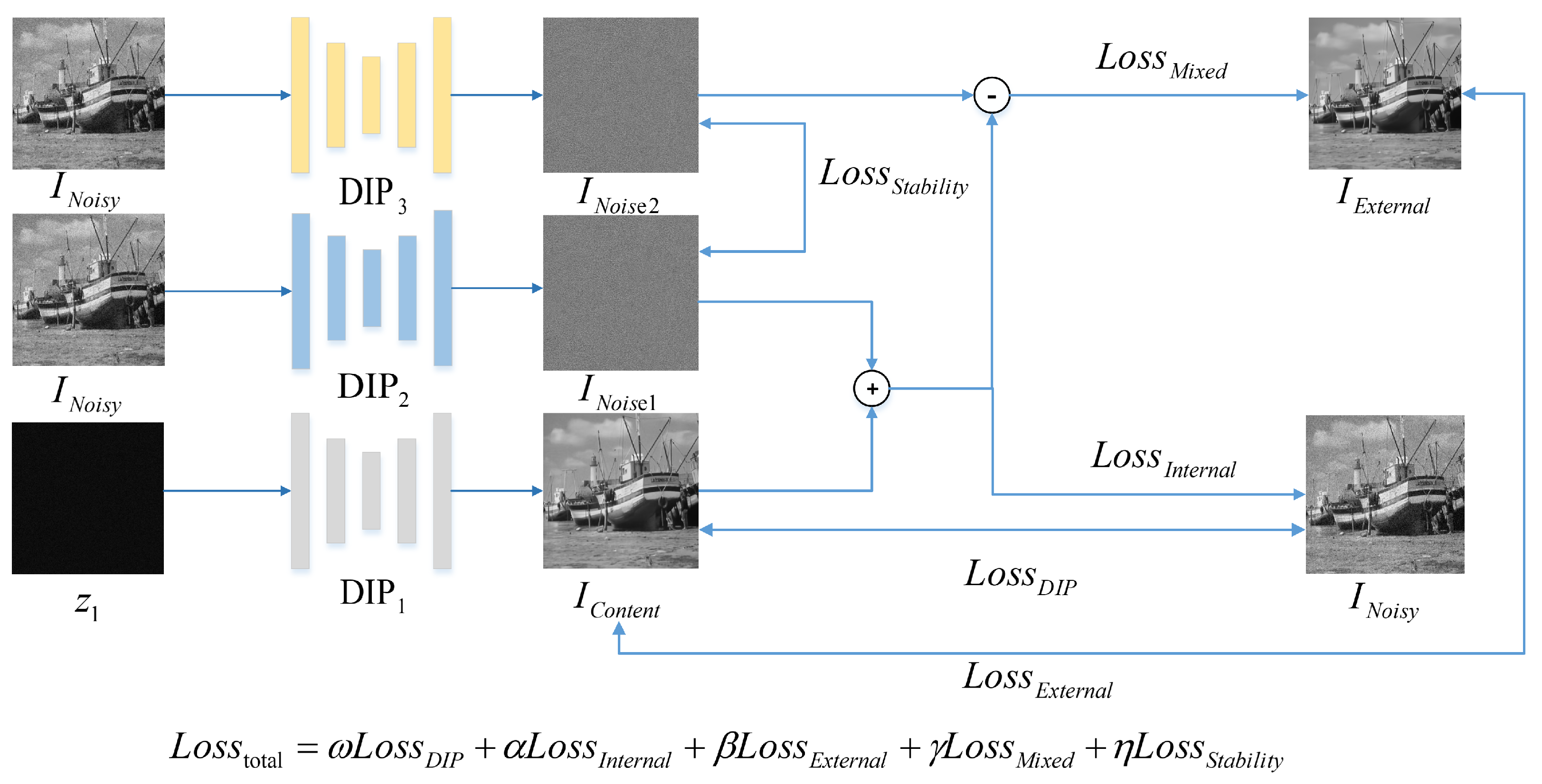
Figure 5.
The average performance of the competitive methods on Set12.

Figure 6.
The average performance of the competitive methods on BSD68.

Figure 7.
Visual denoising results of various methods on Boat image.


Table 1.
Performance comparison of different DIP variants.
| Methods | Number of Iteration | Regularization Method | Noise Learning | Denoising Performance |
|---|---|---|---|---|
| DIP [34] | Fixed | Internal prior (particular network) | without | Baseline |
| DIP-TV [36] | Fixed | Internal prior (total variation) | without | Enhanced |
| DIPRecon [37] | Fixed | Internal prior (similar images) | without | Enhanced |
| DIP-ES [38] | Automatic | Internal and external priors (auto-encoder) | without | Enhanced |
| DeepRED [39] | Fixed | Internal prior (pre-set denoiser) | without | Enhanced |
| PnP-DIP [40] | Fixed | Internal prior (pre-set denoiser) | without | Enhanced |
| TripleDIP | Automatic | Internal and external priors | with | Significant |
Table 2.
The average PSNR results for different preprocessed images.
| Generator | N2V | IRCNN | DnCNN | DeamNet | DAGL | SwinIR | Restormer |
|---|---|---|---|---|---|---|---|
| PSNR | 30.62 | 31.24 | 31.34 | 31.50 | 31.58 | 31.68 | 31.70 |
Table 3.
The average PSNR results for different weights of .
| 0.1 | 0.2 | 0.3 | 0.4 | 0.5 | 0.6 | |
|---|---|---|---|---|---|---|
| PSNR | 31.32 | 31.40 | 31.61 | 31.70 | 31.63 | 31.51 |
Table 4.
The average PSNR results for different network structures. The checkmark means it was used in the loss function or network input.
Table 4.
The average PSNR results for different network structures. The checkmark means it was used in the loss function or network input.
| Structure | Loss Function | Noisy Branch Input | Avg (dB) | |||||
|---|---|---|---|---|---|---|---|---|
| SingleDIP | ✔ | ✔ | 31.56 | |||||
| DoubleDIP1 | ✔ | ✔ | ✔ | ✔ | 31.52 | |||
| DoubleDIP2 | ✔ | ✔ | ✔ | ✔ | 31.53 | |||
| TripleDIP1 | ✔ | ✔ | ✔ | ✔ | ✔ | ✔ | 31.53 | |
| TripleDIP2 | ✔ | ✔ | ✔ | ✔ | ✔ | ✔ | ✔ | 31.55 |
| TripleDIP | ✔ | ✔ | ✔ | ✔ | ✔ | ✔ | 31.70 | |
Table 5.
The average PSNR and SSIM values of competitive methods on Set12 with different noise levels.
Table 5.
The average PSNR and SSIM values of competitive methods on Set12 with different noise levels.
| Method | Avg | |||
|---|---|---|---|---|
| BM3D | 32.36/0.95 | 29.96/0.92 | 26.70/0.87 | 29.67/0.91 |
| DnCNN | 32.67/0.95 | 30.35/0.93 | 27.18/0.88 | 30.07/0.92 |
| FFDNet | 32.75/0.95 | 30.43/0.93 | 27.32/0.88 | 30.17/0.92 |
| DIP | 31.33/0.94 | 28.95/0.90 | 25.52/0.83 | 28.60/0.89 |
| N2V | 30.86/0.88 | 29.46/0.91 | 25.83/0.73 | 28.71/0.84 |
| VDNet | 30.05/0.93 | 29.33/0.92 | 27.73/0.89 | 29.04/0.91 |
| WINNet | 32.85/—– | 30.54/—– | 27.40/—– | 30.26/—– |
| BCDNet | 33.01/—– | 30.75/—– | 27.65/—– | 30.47/—– |
| DAGL | 33.19/0.96 | 30.86/0.94 | 27.75/0.89 | 30.60/0.93 |
| DeamNet | 33.13/0.96 | 30.78/0.94 | 27.72 /0.89 | 30.55/0.93 |
| DRUNet | 33.25/0.96 | 30.94/0.94 | 27.90/0.89 | 30.69/0.93 |
| IRCNN | 32.76/0.95 | 30.37/0.93 | 27.12 /0.88 | 30.08/0.92 |
| Restormer | 33.35/0.96 | 31.04/0.94 | 28.01/0.90 | 30.80 /0.93 |
| SwinIR | 33.36/0.96 | 31.01/0.94 | 27.91/0.89 | 30.76/0.93 |
| TripleDIP | 33.98/0.96 | 31.70/0.94 | 28.50/0.90 | 31.39/0.93 |
Table 6.
The average PSNR and SSIM values of competitive methods on BSD68 with different noise levels.
Table 6.
The average PSNR and SSIM values of competitive methods on BSD68 with different noise levels.
| Method | Avg | |||
|---|---|---|---|---|
| BM3D | 31.15/0.93 | 28.57/0.88 | 25.58/0.80 | 28.43/0.87 |
| DnCNN | 31.62/0.94 | 29.14/0.90 | 26.18/0.82 | 28.98/0.89 |
| FFDNet | 31.65/0.94 | 29.17/0.90 | 26.24/0.83 | 29.02/0.89 |
| DIP | 30.03/0.92 | 27.47/0.87 | 24.26/0.78 | 27.25/0.86 |
| N2V | 29.38/0.85 | 27.81/0.87 | 25.37/0.67 | 27.52/0.80 |
| VDNet | 28.65/0.89 | 27.90/0.87 | 26.45/0.84 | 27.67/0.87 |
| WINNet | 31.70/—– | 29.27/—– | 26.36/—– | 29.11/—– |
| BCDNet | 31.81/—– | 29.37/—– | 26.47/—– | 29.22/—– |
| DAGL | 31.81/0.94 | 29.33/0.90 | 26.37/0.83 | 29.17/0.89 |
| DeamNet | 31.83/0.94 | 29.35/0.91 | 26.42 /0.83 | 29.20/0.89 |
| DRUNet | 31.86/0.94 | 29.39/0.91 | 26.49/0.84 | 29.25/ 0.89 |
| IRCNN | 31.65/0.94 | 29.13/0.90 | 26.14 /0.82 | 28.97/0.89 |
| Restormer | 31.88/0.94 | 29.41/0.91 | 26.49/0.84 | 29.26/0.90 |
| SwinIR | 31.91/0.94 | 29.41/0.91 | 26.47/0.84 | 29.26/0.89 |
| TripleDIP | 32.24/0.94 | 30.22/0.92 | 26.92/0.84 | 29.79/0.90 |
Disclaimer/Publisher’s Note: The statements, opinions and data contained in all publications are solely those of the individual author(s) and contributor(s) and not of MDPI and/or the editor(s). MDPI and/or the editor(s) disclaim responsibility for any injury to people or property resulting from any ideas, methods, instructions or products referred to in the content. |
© 2023 by the authors. Licensee MDPI, Basel, Switzerland. This article is an open access article distributed under the terms and conditions of the Creative Commons Attribution (CC BY) license (https://creativecommons.org/licenses/by/4.0/).
Share and Cite
MDPI and ACS Style
Hu, Y.; Xu, S.; Cheng, X.; Zhou, C.; Hu, Y. A Triple Deep Image Prior Model for Image Denoising Based on Mixed Priors and Noise Learning. Appl. Sci. 2023, 13, 5265. https://doi.org/10.3390/app13095265
AMA Style
Hu Y, Xu S, Cheng X, Zhou C, Hu Y. A Triple Deep Image Prior Model for Image Denoising Based on Mixed Priors and Noise Learning. Applied Sciences. 2023; 13(9):5265. https://doi.org/10.3390/app13095265
Chicago/Turabian StyleHu, Yong, Shaoping Xu, Xiaohui Cheng, Changfei Zhou, and Yufeng Hu. 2023. "A Triple Deep Image Prior Model for Image Denoising Based on Mixed Priors and Noise Learning" Applied Sciences 13, no. 9: 5265. https://doi.org/10.3390/app13095265
Note that from the first issue of 2016, this journal uses article numbers instead of page numbers. See further details here.