Method for Training and White Boxing DL, BDT, Random Forest and Mind Maps Based on GNN

Abstract

A method for training and white boxing of deep learning (DL) binary decision trees (BDT), random forest (RF) as well as mind maps (MM) based on graph neural networks (GNN) is proposed. By representing DL, BDT, RF, and MM as graphs, these can be trained by GNN. These learning architectures can be optimized through the proposed method. The proposed method allows representation of the architectures with matrices because the learning architecture can be expressed with graphs. These matrices and graphs are visible, which makes the learning processes visible, and therefore, more accountable. Some examples are shown here to highlight the usefulness of the proposed method, in particular, for learning processes and for ensuring the accountability of DL together with improvement in network architecture.

1. Introduction

One of the major problems of DL is the black box problem which means DL has no accountability and that the logic in the DL is not transparent. There are three major problems with DL:

(1)

The black box problem;

(2)

The bias problem in which the output of the DL includes biases if training datasets includes biases;

(3)

Weakness against noise.

Things that are difficult for humans to understand as explicit rules are known as so-called black box problems. In contrast to the conventional (deductive) system development method of writing programs (procedures), the system development method (inductive type) using machine learning by exemplifying data ensures safety and reliability. Attempts are being made to solve the black box problem by exploring the different methodologies and technology systems that can be used.

In machine learning, with methods such as decision trees and linear regression, the regularity of training results (rules and models) can be obtained in a form that is easy for humans to understand (if-then rules, linear sum formulas, etc.). Avoiding the black box problem is a trade-off between accuracy and interpretability, which is difficult to achieve at the same time.

The following three methods are being considered as methods of giving interpretability to machine learning.

(1)

Deep Explanation: Attention heat map and natural language explanation generation by deep learning state analysis, etc.

(2)

Interpretable Models: Machine learning using models that are originally highly interpretable (improving the accuracy of white box type machine learning),

(3)

Model Induction: Creating an external, highly interpretable model that approximates the behavior of black box machine learning.

In order to make clear the logic in the DL, a multistage DL is proposed. Namely, the whole process is divided into several stages. Then, interim results from each stage of the DL make processes of the whole DL learning processes interpretable. Some examples of multistage DLs have already been demonstrated. For instance, in order to understand the growth situation of rice in paddy fields, to estimate the yield and quality of harvested rice, that is, the protein content of brown rice, a drone mounted Normalized Difference Vegetation Index (NDVI) camera data were used as input data, and the desired outputs were the yield and protein content of brown rice as training data [1].

When the model is learning as a set and estimating the yield and quality using unknown NDVI image data as input, estimations can be obtained, but it is not known on what logic the results are generated, making it a so-called black box problem. In order to solve this problem, DLs are applied in the following three stages:

(1)

The period from rice planting until the ear emerges,

(2)

The stage when the ear of rice has fully grown,

(3)

The stage just before harvesting.

In this example, by applying DL to each stage and learning with the different training datasets, the estimation results can be explained from the intermediate results of each stage.

The proposed method allows solving the black box problem based on GNN [2,3] and GCN. The proposed method also allows training of random forest types of classification methods based on GNN and GCN. GNN and GCN allow the construction of learning models with graphs which are a process flow form of data analysis. For instance, the decision tree type of discrimination can be written in a form of graph with and/or without directions. The graphs can be rewritten with matrices. Then the matrices can be input to DLs. Thus, the process flow can be learned by the DLs.

On the other hand, by representing DL, BDT, RF, and MM as graphs, they can be trained by GNN. These learning architectures can be optimized through the proposed method which allows the architectures to be represented with matrices because the learning architecture can be expressed with graphs. Graph HyperNetworks for neural architecture search have been investigated [4]. These matrices and graphs are visible, thereby making the learning processes visible so that the results in the learning processes become transparent.

In the next section, related research works are reviewed and the proposed methodology is outlined. Some examples are described, followed by a discussion and conclusion.

2. Previous Works

Graph theory itself is said to have started when Euler introduced it to one-stroke problems such as the Seven Bridges of Königsberg. It is a field that is widely applied. A graph is a data structure represented by objects (nodes) and relationships (edges) between them. On the other hand, deep learning has mainly dealt with collections of individual data (vectors), data arranged in grids (images), and sequential data (text, voice). Therefore, it is a natural step to incorporate graph theory into DL and develop it.

On the other hand, from the point of view of representation learning, nodes, edges, and subgraphs with low-dimensional vectors can be represented. In the area of graph analysis, traditional methods of machine learning rely on manually setting feature values, whereas graph-embedded methods can learn. DeepWalk, Skipgram model, node2vec, LINE, and TADW are some examples [5,6,7,8,9,10,11,12,13,14,15,16,17,18]. However, this approach also has its drawbacks: it is inefficient because parameters are not shared between nodes, and direct embedding lacks the ability to generalize.

The matrix representation for treating graphs mathematically is as follows:

(1)

Adjacency matrix A expresses whether there is a connection relationship between nodes.

(2)

The degree matrix D represents how many edges are connected to each node.

The Laplacian matrix is a representation of these together: L = D − A, as shown in Figure 1. A normalized Laplacian matrix is actually used.

There are the following three types of networks:

(1)

Graph Recurrent Networks (recurrent networks)

In an early proposed model, information propagation is performed recursively using the same function. However, the low computational efficiency is considered a problem.

(2)

Graph Convolutional Networks (convolutional network, hereinafter referred to as GCN)

GCN is a proposed model that is based on the mechanism of CNN, but parallel calculation is possible, so calculation efficiency is improved. Considering the type of convolution, these models can be divided into two types: the spectral method and spatial method. The former treats graphs as signal processing. The latter is more popular than the former because it is defined based on the relationships of the graph itself and is more intuitive than the former.

(3)

Graph Attention Networks (Attention-based networks)

This model applies the mechanism of “Attention” to GNN.

In the GCN model of (2), the node relationships are treated with the same importance, but by introducing “Attention”, it is possible to assign importance scores to relationships, enabling more flexible judgment.

Since GNN handles data composed of nodes and edges, it can be said that it is most suitable for processing objects that can be expressed in this format. For example, it is Thewidely applied in fields such as social network prediction, traffic/logistics prediction, recommendation systems, and compound/biomolecular analysis. Furthermore, even for data that cannot be expressed directly in graph form, such as document text, it is possible to use GNN by incorporating graphs of other areas (e.g., knowledge graphs) and applying them by assuming relationships.

At the North American Chapter of the Association for Computational Linguistics (NAACL) international conference, many studies using GNN were presented. For example, some of the participants applied an utterance relation graph and an action graph to the abstract summarization of a conversation to reveal the structure of the conversation [19] or applied the GCN to sentiment analysis to reveal each aspect of the analyzed document. A model based on this GCN has been proposed [20].

Graph Neural Network processing is divided into three stages: aggregation of adjacent nodes (AGGREGATE), updating by aggregation of results (COMBINE), and aggregation of node features to obtain properties of the entire graph (READOUT). In order to compare the similarity of graphs, one method is to assign a label to each type of node connection and count and compare their number (Weisfeiler–Lehman Graph Isomorphism Test) [21,22]. In this context, things with the same connections should have the same label, and things with different connections should have different labels (injective). Therefore, it is necessary to pay attention not to break injectivity in various places of AGGREGATE/COMBINE/READOUT.

If MEAN and MAX with AGGREGATE are taken, then cases where the number of connections is different, but the MEAN/MAX are the same can be distinguished (it is acceptable with SUM because it increases with the number of connections). However, this is not the case when the number of connections is too large or when removal of noise (such as a 3D point cloud) is required, or when the distribution of connected nodes is important rather than the connection structure. Surprisingly, SUM was preferable because it was the same as the result when text classification was tried. In that paper, a simple SUM-based Graph Neural Network (Graph Isomorphism Network (GIN)) was created based on this theory [23], and achieved scores equal to or better than SOTA (Summits on The Air Database [24]) on various datasets.

GNNs are primarily intended for node classification or graph classification. To do this, the node/graph representation is computed, which can be divided into the following three steps:

(1)

AGGREGATE: Aggregate information of neighboring nodes;

(2)

COMBINE: Update node features from the aggregated node information;

(3)

READOUT: Obtain a representation of the entire graph from the nodes in the graph.

For GraphSAGE, AGGREGATE = eLU + Maxpooling after multiplying by the weight and COMBINE = combining after multiplying by the weight. Moreover, for GCN, AGGREGATE = MEAN of adjacent nodes, and COMBINE = ReLU after multiplying by the weight. It seems that READOUT uses total or special pooling.

The core of that paper is the Weisfeiler–Lehman Graph Isomorphism Test (WLGIT). This is a technique for measuring how similar graphs are to each other. Nodes are listed (List), aggregated by connection type (Compress), and a label of aggregation unit (category) is assigned to the node (Relabel). By repeating this, the labels of the updated neighboring nodes will affect the next update, that is, the information of the distant nodes will also be taken into account. This aspect is very similar to Graph Convolution (Neural Network).

If a “unique” label is assigned to those with the same connection, they are relabeled (only one label is assigned to a node of two points). This means that the relationship between nodes and labels is injective. Even in each process of Graph Neural Network, it is not possible to obtain the same discrimination as with Weisfeiler–Lehman unless this constraint is satisfied. The point is that injectivity is lost when aggregation other than SUM is performed. In the case of MAX/MEAN, an indistinguishable graph structure occurs, namely, information about the “number” of connected nodes is dropped (different numbers but same MAX/MEAN cases cannot be distinguished). However, this is not the case if it is intended to reduce the number of pieces of information. Based on this theory, a simple SUM-based Graph Neural Network (Graph Isomorphism Network (GIN)) was created, and achieved scores equal to or better than SOTA on various datasets.

Natural language processing does not attempt to identify sentences by graph structure. In the case of dependencies, it is hard to imagine that text classification results differ depending on the shape of the dependency. The same is true for word similarity. Therefore, it is not necessary to calculate the SUM, which must be aware of the structure of the graph. However, since the number of words is important information, it is considered effective to calculate the SUM at least at the time of READOUT.

Natural language processing does not use graph neural networks for graph classification or node classification. In that sense, it can be considered that only the information of the adjacency matrix is sufficient, and the discriminative power of the Graph Neural Network is not used. If a Graph Neural Network is to be used well, it is necessary to apply it to the graph or node identification problem [25,26].

3. Proposed Method

DL, decision tree, random forest, and mind map models can be expressed as directed graphs and can be represented as matrices. Therefore, these learning processes can be performed with GNN and GCN. The nodes in the hidden layers can be seen so that it becomes visible and transparent. The procedure for white boxing is as follows:

(1)

Make directed graphs of the DL, decision tree, random forest, or mind map;

(2)

Convert the directed graphs to matrices;

(3)

Use these matrices as input of the training samples of GNN and GCN;

(4)

Visualize the node in the hidden layers of the GNN and GCN, which results in white boxing of DL and the other models.

The image is processed as local data separated by grids, and several layers of CNN are superimposed to grasp the overall image of the object. In the graph, Euclidean distance is not relevant, and the data points related to the object are combined and treated as a data set. The adjacency matrix A expresses whether or not there is a connection relationship between nodes, and the degree matrix D expresses how many edges are connected to each node. In addition, the Laplacian matrix is a representation of these together: a normalized Laplacian matrix obtained by normalizing the L = D-Laplacian matrix is actually used.

A graph is a data structure in which nodes (vertices) are connected by edges (branches) that represent adjacency relationships. Graphs can be represented mathematically by matrices, and this GCN uses the following two matrices: the aforementioned adjacency matrix and a feature matrix:

(1)

Adjacency matrix: a matrix that represents the connection relationship between nodes.

(2)

Feature Matrix: a matrix representing the feature vector of each node.

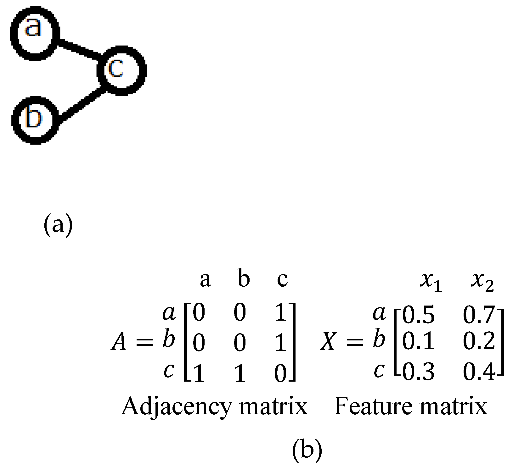
The example in the following figure (Figure 2) can be represented by an adjacency matrix and a feature matrix.

Orange letters represent each node. For example, in the adjacency matrix, the third column of the first row contains 1 because node “a” and node “c” are connected. In the feature matrix, x₁ and x₂ indicate features, as shown in Figure 2.

GCNs are techniques for applying deep learning to graph data. GCN is a convolutional neural network that quantifies each node with structure. Taking into account the structure means that the node’s focusing point is digitized and takes into account what kind of node it is attached to.

Let G = (V, E, X) denote an undirected and unweighted graph comprising a set of nodes V, a set of edges E, and a set of node feature vectors X = {x₁, …, x_n} corresponding to nodes in V, where x_u$\in$R^M. Let n = |V| denote the number of nodes in the graph and A $\in$ R^n×n be the adjacency matrix (Equation (1)), where element A_ij = 1 if nodes i and j are connected by some edge in E, and A_ij = 0 otherwise. As the input data of GCN, the following two matrices are used.

3.1. Input

(1)

Adjacency matrix:

$$A\in R^{n\times n}A$$

(1)

This matrix that shows which nodes are connected to which nodes. Namely, A is defined in the n-by-n of R space.

(2)

Feature Matrix:

$$F_{in}\in R^{n\times \left|F\right|}A$$

(2)

This matrix represents the feature vector of each node. In addition, F_in is defined in the n by |F| space.

3.2. Output

(1)

Latent Matrix:

$$H_{out}\in R^{n\times \left|H\right|}A$$

(3)

This matrix represents the latent expression vector of each node (converted by GCN). Namely, H_out is defined in the n by |H| space.

3.3. Formula

GCN can be expressed with the following formula:

$$H^{\left(l+1\right)}=f\left(H^{\left(l\right)},A\right)$$

(4)

where $H^{\left(0\right)}=X.$ For instance, taking a one-layer GCN with activation function ReLU as an example, W is a weight as in a normal neural network. A, X are the adjacency matrix and feature matrix (input), respectively.

$$f\left(H^{\left(0\right)},A\right)=f\left(X,A\right)=ReLU\left(AX·W\right)$$

(5)

In other words, AX can be seen as the adjacency matrix by feature matrix that is the sum of the feature values of the nodes connected to a certain node. With AX, the feature value considering the surrounding nodes can be obtained. Then, it simply multiplies AX by the weight W and applies the nonlinear activation function ReLU like a normal neural network.

GCN can be regarded as a special case of the Weisfeiler–Lehman algorithm with (1) parameters and (2) differentiability.

3.4. Mind Map

Mind mapping is a method of expressing thoughts devised by British author and educator Tony Buzan and is used around the world as a form of notetaking that makes use of the natural functions of the brain.

Tony Buzan has trademarked “Mind Map” not only in English but also in Japanese. His original mind map is a natural expression of thoughts that makes use of the characteristics of the brain. Therefore, it enhances creativity and is highly effective in memory, learning, and thinking. It is a very effective method that can exploit the brain’s inherent abilities. Only authorized instructors with Tony Buzan’s license can correctly convey the concepts of these mind maps.

3.5. Decision Tree to Random Forest

Decision tree analysis (decision tree) is an analysis method that uses a tree structure to classify data and extract patterns. In addition to pattern extraction in the fields of machine learning and statistics, it is used in marketing to discover factors that affect target selection and customer satisfaction.

Decision tree analysis uses a tree-like dendrogram to classify data. For example, if it is necessary to identify the market segment that purchases product “A” the most on an e-commerce site, the customer data are classified as shown in the figure above. First, the objective variable is set. The objective variable is an item that greatly affects the results of decision tree analysis.

For example, to find the customer segment of buyers, “buy/non-purchase of product “A” is used as the objective variable. Next, the data are branched by explanatory variables and classified. The results of the explanatory variables can then be checked. In another example, the customers are divided by “gender”, “place of residence”, and “age”, and it is found, for instance, that the largest number of purchasers are “male, living in the metropolitan area, 39 years old or younger”.

Decision tree analysis can be used for exploring the factors that affect it by clarifying the explanatory variables that affect the set objective variable.

3.6. Random Forest

“Random forest” is a type of ensemble learning using decision trees that is a well-known and widely used model. It can be used for class classification, regression, clustering, etc. This method uses multiple decision trees and obtains results by majority vote of the prediction results of each decision tree. This kind of learning method using multiple models to improve performance is called ensemble learning and it is widely used in addition to random forests.

Random Forest creates decision trees by randomly selecting data samples, obtains predictions from each tree, and chooses the best solution by voting. For example, if five decision trees are created and three out of five are “A” and two are “B”, then “A” is selected. This is called “majority logic”. In addition, when it comes to regression problems, if five are predicted to be [4,8,10,12,14], it will be predicted with a mean of 9.6 and a median of 10.

Random forests have various applications such as recommendation engines, image classification, and feature selection. Therefore, it is a highly accurate and popular algorithm.

The four steps of the algorithm are:

(1)

Select a random sample from the given dataset;

(2)

Build a decision tree for each sample and obtain a prediction result from each decision tree;

(3)

Vote for each prediction result;

(4)

Select the prediction result with the most votes as the final prediction.

The advantages of the random forest algorithm are as follows:

(1)

In random forests, each decision tree has different characteristics and can make complex decisions;

(2)

Compared with decision trees, there is no problem of overfitting. The main reason is the average of all predictions is taken to cancel out the bias;

(3)

Random forest can also handle missing values. There are two ways to handle these: using the median value to replace the continuous variable and computing the proximity-weighted average of the missing values;

(4)

Importance can be obtained. This helps select the features that contribute the most to the classifier.

On the other hand, the disadvantages of this algorithm are as follows:

(1)

Random forests are slow to generate predictions due to multiple decision trees. For every prediction, every tree in the forest must make a prediction on the same input and perform a vote on it. This entire process takes time.

(2)

Compared with decision trees, the models are harder to interpret because there are multiple trees.

3.7. Proposed Method

The method proposed here is to use GCN for training processes of the random forest in order to overcome the aforementioned disadvantages. The random forest can be represented in samples of tree structures which are expressed as graphs. Therefore, the random forest can be trained by GCN. DL can also be represented as graphs. Therefore, it can be trained with GCN. Because the DL has the so-called “black box problem”, the output of the DL cannot be transparent. If the GCN is used for the training processes of the DL, then it becomes transparent because the hidden layer nodes can be seen clearly using GCN. Thus, the black box problem can be solved.

Furthermore, mind maps can be represented with GCN and can, therefore, be trained. This implies that expertise can be transferred or promulgated within a GCN.

4. Examples

4.1. Application of the Proposed Method for Decision Tree Based Discrimation Method

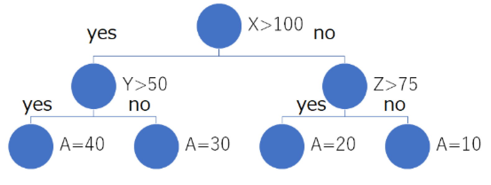
Figure 3 shows an example of the decision-tree-based discrimination method.

This tree structure can be represented with a directional graph which results in a matrix. The decision tree can be expressed with directed graph as follows:

G = (V, E)

(6)

where vertex set V and edge set E represent an ordered pair of vertices, e = (u, v), vertex u is the start point of branch e, and vertex v is the end point of branch e. For instance, Figure 4a of the directed tree can be represented with Figure 4b of the matrix.

Then, the matrix can be an input of the GNN and GCN. Therefore, it can be trained with GNN and GCN. The same applies for the random forest type of discrimination method. In the GNN and GCN, the interim results in the hidden layer nodes can be seen and visualized. Therefore, the learning processes in GNN and GCN can be transparent.

4.2. Application for Mind Map Learning Method

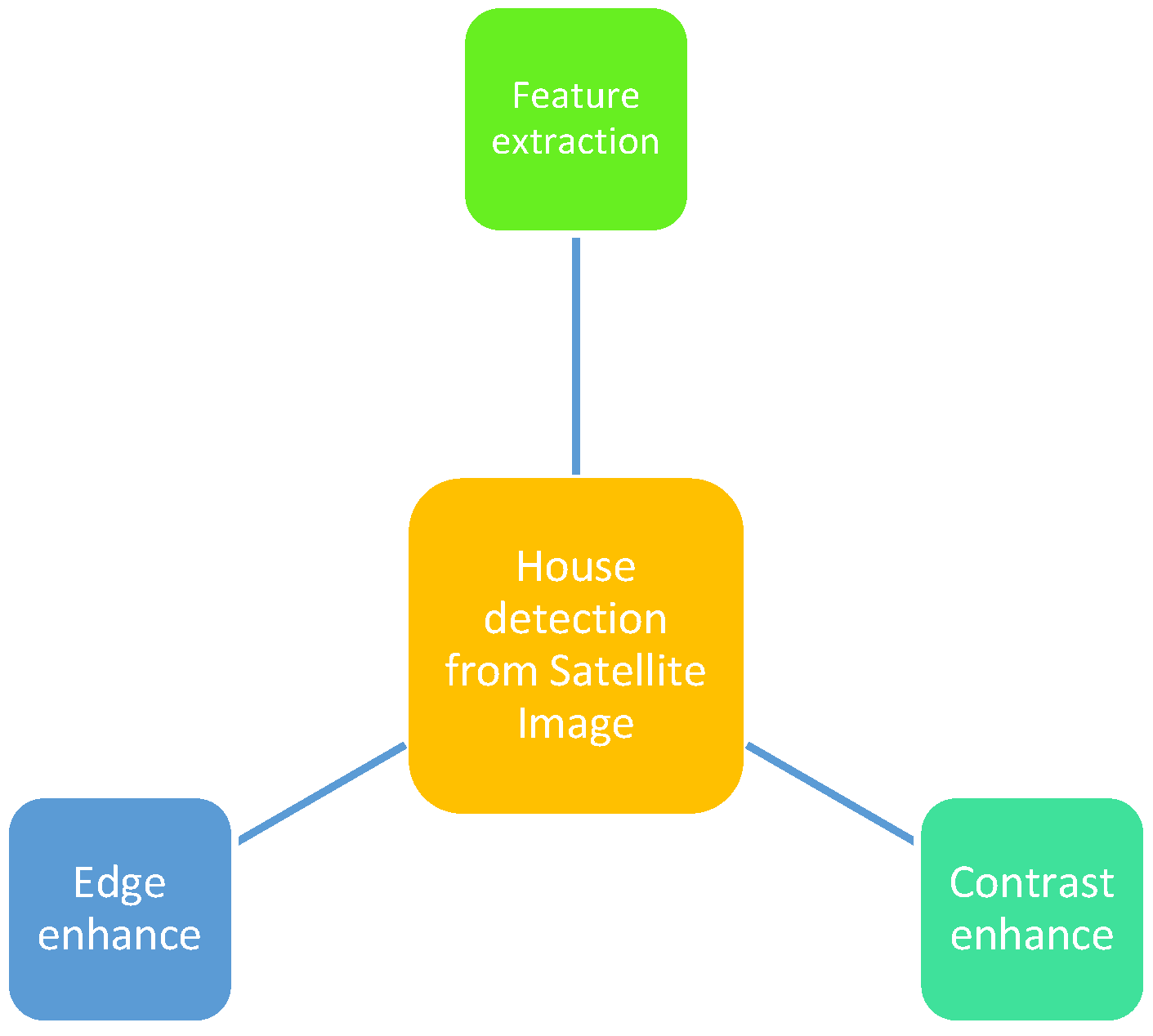
Another example is a mind map. Figure 5 shows the example of a mind map used for house detection from remote sensing satellite images.

Mind maps can be represented as matrices and, therefore, can be trained by GNN and GCN. The most appropriate process flow can be learned through learning processes of GNN and GCN.

4.3. Application for Random Forest Based Discrimination Method

The Random Forest-Based Discrimination (RFBD) method can be described with matrices, which results in the proposed method that can be used for RFBD learning processes, as shown in Figure 6. In Figure 6, majority logic means that the final output result is determined by the majority of the outputs of a plurality of decision trees.

4.4. Representation of CNN Architecture with Graphs

A simple example of how a CNN architecture can be represented as a graph is as follows:

 

import torch

from torch_geometric.data import Data

 

# Define the CNN model architecture

class CNN(torch.nn.Module):

def __init__(self, input_dim, output_dim):

super(CNN, self).__init__()

self.conv1 = torch.nn.Conv2d(input_dim [0], 16, kernel_size = 3, stride = 1, padding = 1)

self.pool1 = torch.nn.MaxPool2d(kernel_size = 2, stride = 2)

self.conv2 = torch.nn.Conv2d(16, 32, kernel_size = 3, stride = 1, padding = 1)

self.pool2 = torch.nn.MaxPool2d(kernel_size = 2, stride = 2)

self.linear1 = torch.nn.Linear(32 * 7 * 7, 256)

self.linear2 = torch.nn.Linear(256, output_dim)

 

def forward(self, x):

x = self.conv1(x)

x = torch.relu(x)

x = self.pool1(x)

x = self.conv2(x)

x = torch.relu(x)

x = self.pool2(x)

x = x.view(x.size(0), −1)

x = self.linear1(x)

x = torch.relu(x)

x = self.linear2(x)

return x

 

# Define a function to generate the graph representation of the CNN architecture

def generate_graph(input_dim, output_dim):

nodes = [

(‘conv1′, torch.tensor([1, 1, 3, 3])),

(‘pool1′, torch.tensor([2, 2, 2, 2])),

(‘conv2′, torch.tensor([1, 16, 3, 3])),

(‘pool2′, torch.tensor([2, 2, 2, 2])),

(‘linear1′, torch.tensor([32 * 7 * 7, 256])),

(‘linear2′, torch.tensor([256, output_dim]))

]

edges = [

(‘conv1′, ‘pool1′),

(‘pool1′, ‘conv2′),

(‘conv2′, ‘pool2′),

(‘pool2′, ‘linear1′),

(‘linear1′, ‘linear2′)

]

node_names = [node [0] for node in nodes]

node_shapes = [node [1] for node in nodes]

node_indices = [sum(node_shapes[:i]) for i in range(len(node_shapes))]

edge_indices = [(node_names.index(edge [0]), node_names.index(edge [1])) for edge in edges]

x = torch.tensor([[1.], [0.], [0.], [0.], [0.], [0.]])

edge_index = torch.tensor(edge_indices, dtype = torch.long).t().contiguous()

return Data(x = x, edge_index = edge_index)

 

In this example, the CNN architecture is defined using PyTorch, and a graph representation of the architecture is generated using the generate_graph function. The nodes of the graph represent the different layers of the CNN (e.g., conv1, pool1, etc.), and the edges represent the connections between the layers. The x tensor contains the initial node features, which in this case is set to [1., 0., 0., 0., 0., 0.], indicating that the first node (corresponding to the first layer) is the starting point for traversing the graph. The edge_index tensor contains the indices of the nodes that are connected by each edge.

4.5. Representation of CNN Architecture with Matrices

To plot the adjacency matrix of the graph of a CNN, it is possible to use the nx.to_numpy_matrix() function from the NetworkX library in Python. The example code is as follows:

 

import networkx as nx

import matplotlib.pyplot as plt

import numpy as np

 

# Define the CNN architecture

model = nx.DiGraph()

model.add_node(‘Input’)

model.add_node(‘Conv1′)

model.add_node(‘MaxPool1′)

model.add_node(‘Conv2′)

model.add_node(‘MaxPool2′)

model.add_node(‘Flatten’)

model.add_node(‘Dense1′)

model.add_node(‘Dense2′)

model.add_node(‘Output’)

 

model.add_edge(‘Input’, ‘Conv1′)

model.add_edge(‘Conv1′, ‘MaxPool1′)

model.add_edge(‘MaxPool1′, ‘Conv2′)

model.add_edge(‘Conv2′, ‘MaxPool2′)

model.add_edge(‘MaxPool2′, ‘Flatten’)

model.add_edge(‘Flatten’, ‘Dense1′)

model.add_edge(‘Dense1′, ‘Dense2′)

model.add_edge(‘Dense2′, ‘Output’)

 

# Generate the adjacency matrix

adj_matrix = nx.to_numpy_matrix(model)

 

# Plot the adjacency matrix

plt.imshow(adj_matrix, cmap = ‘binary’)

plt.title(‘Adjacency Matrix of CNN’)

plt.xticks(range(adj_matrix.shape [0]), model.nodes())

plt.yticks(range(adj_matrix.shape [0]), model.nodes())

plt.show()

 

This will generate a visualization of the adjacency matrix using the matplotlib library.

4.6. White Boxing of Deep Learning

Because the matrix elements in the GCN and GNN can be seen, the deep learning processes can be visualized. All nodes in deep learning have features, and these nodes can be represented as graphs, that is, matrices, so the learning process can be visualized. In order to train the model, a definition of the loss function is needed in the embedding process. The embedding process should be fed into any loss function and a stochastic gradient descent is then performed to train the weight parameters.

Graph visualization is the area of mathematics and computer science where geometric graph theory and information visualization intersect. It has to do with visual representations of graphs that reveal structures and anomalies that may exist in the data and help users understand the graph. Therefore, white boxing can be performed for all types of machine learning including deep learning, with the result that machine learning becomes accountable.

In deep learning, a neural network can be represented using a graph structure. This graph is known as a computational graph or a neural network graph. The nodes of the graph represent the computations that are performed, while the edges represent the flow of data between these computations.

Each node in the graph represents a mathematical operation or transformation on the input data. These operations can include linear transformations, non-linear activation functions, pooling operations and more. The inputs to a node are the outputs of the previous nodes, and the output of a node becomes the input to the next node in the graph.

The graph can be represented using different frameworks or libraries, such as TensorFlow, PyTorch, or Keras. These frameworks provide a high-level interface to build and train neural networks, while also allowing for low-level customization of the graph structure and computations.

The graph structure of a neural network allows for efficient computation on hardware accelerators such as GPUs or TPUs. By optimizing the graph structure and computation, it is possible to improve the performance and efficiency of deep learning models.

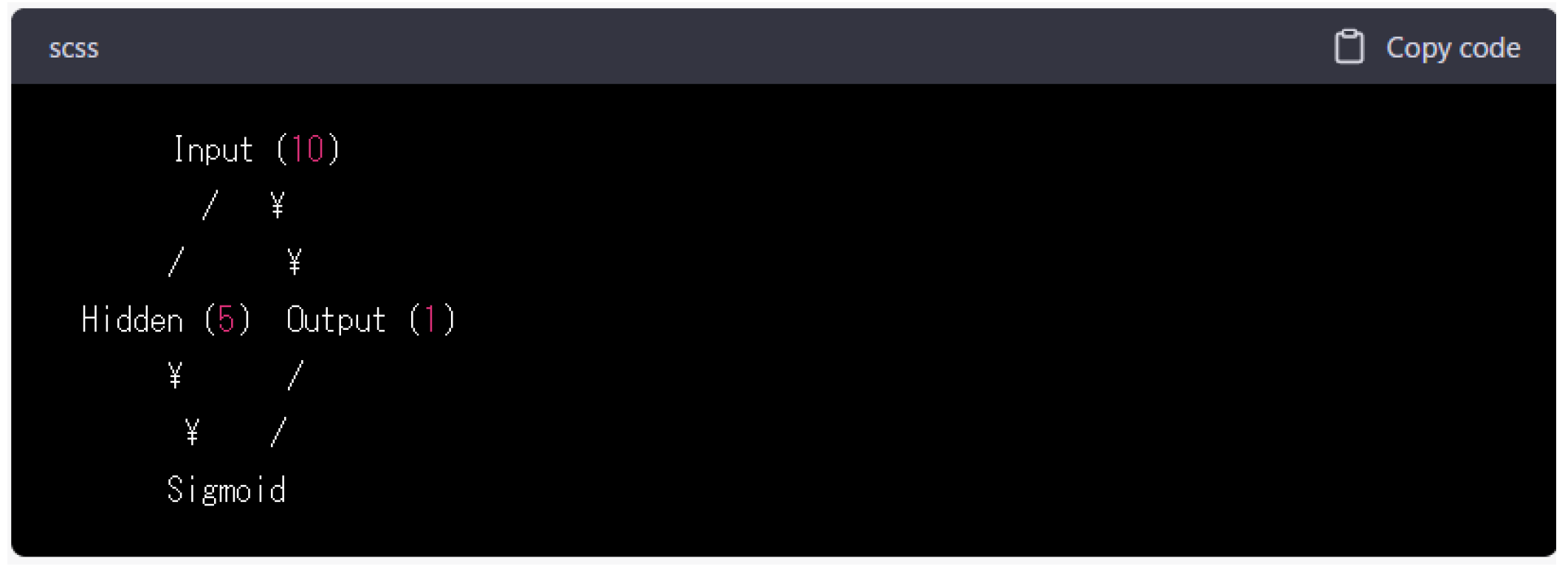
Considering a simple example of a fully connected neural network with one hidden layer, the input to the network is a vector of size 10, and the output is a scalar value. The hidden layer has five neurons and uses a sigmoid activation function. An example of the graph representation of this network can be described as follows.

In this graph, the input node has 10 incoming edges, one for each element in the input vector. The Hidden node has five incoming edges, one for each neuron in the previous layer. The Output node has one incoming edge from the Hidden node. The Sigmoid node represents the activation function applied to the output of the Hidden node.

During the forward pass of this network, the input data flows through the graph, and each node performs its computation. The output of the final node is then compared with the desired output during the training process, and the network parameters are adjusted to minimize the error.

Figure 7 is just a simple example, and more complex neural networks can have many layers and different types of nodes. However, the basic principles of the graph representation remain the same, with each node performing a computation and the data flowing through the edges of the graph.

Graph representations of deep learning can be expressed with GNNs. GNNs are a type of deep learning model that can operate directly on graph-structured data.

In a GNN, the nodes in the graph represent the features or attributes of the data, and the edges represent the relationships or interactions between these features. GNNs operate by passing messages or information between neighboring nodes in the graph, using learnable functions or layers to transform this information.

GNNs can be used for a variety of tasks on graph-structured data, including node classification, link prediction, and graph classification. GNNs have been applied to a wide range of domains, such as social networks, bioinformatics, and recommendation systems.

The graph representation of a deep learning model can be converted into a GNN by defining the graph structure and the node features, and then using GNN layers to perform the computations. This allows for the integration of the graph structure into the model and can improve the performance and interpretability of the model on graph-structured data.

While the use of GNNs can help improve the interpretability of deep learning models on graph-structured data, it is important to note that deep learning models, in general, can still be considered as black boxes.

The reason for this is that deep learning models can have a large number of parameters and non-linear operations, making it difficult to fully understand how they arrive at their predictions or decisions. This is particularly true for tasks such as image or speech recognition, where the features learned by the model can be difficult to interpret.

However, the use of techniques such as GNNs, attention mechanisms, and explainable AI can help improve the interpretability of deep learning models to some extent. These techniques can provide insights into which parts of the input data are most relevant for the model’s decision and can help identify potential biases or errors in the model’s predictions.

In addition, the accountability of deep learning models can be improved through the use of transparency and regulation. This can include the use of open-source software, standardized evaluation metrics, and ethical guidelines for the use of AI. By promoting transparency and accountability in the development and use of deep learning models, we can help ensure that they are used in a responsible and trustworthy manner.

Here is an example program code for training a deep learning model with a GNN using PyTorch:

 

import torch

from torch.nn import Linear

import torch.nn.functional as F

from torch_geometric.nn import GCNConv

 

class GNN(torch.nn.Module):

def __init__(self, num_features, num_classes):

super(GNN, self).__init__()

self.conv1 = GCNConv(num_features, 16)

self.conv2 = GCNConv(16, num_classes)

 

def forward(self, x, edge_index):

x = F.relu(self.conv1(x, edge_index))

x = F.dropout(x, training = self.training)

x = self.conv2(x, edge_index)

return F.log_softmax(x, dim = 1)

 

device = torch.device(‘cuda’ if torch.cuda.is_available() else ‘cpu’)

model = GNN(num_features, num_classes).to(device)

data = data.to(device)

 

optimizer = torch.optim.Adam(model.parameters(), lr = 0.01, weight_decay = 5e−4)

criterion = torch.nn.NLLLoss()

 

def train():

model.train()

optimizer.zero_grad()

out = model(data.x, data.edge_index)

loss = criterion(out[data.train_mask], data.y[data.train_mask])

loss.backward()

optimizer.step()

return loss

 

def test():

model.eval()

with torch.no_grad():

out = model(data.x, data.edge_index)

pred = out.argmax(dim = 1)

acc = pred.eq(data.y[data.test_mask]).sum().item()/data.test_mask.sum().item()

return acc

 

for epoch in range(1, 201):

loss = train()

acc = test()

print(f’Epoch {epoch}, Loss: {loss:.4f}, Test Accuracy: {acc:.4f}’)

 

This code defines a GNN model with two GCNConv layers and trains it using the Adam optimizer and NLLLoss criterion. The train() and test() functions handle the training and testing of the model, respectively.

Note that this code assumes that the graph data has already been loaded into a PyTorch Geometric Data object (called data in the code), which contains the node features, edge indices, and train/test masks. It is necessary to modify the code accordingly to suit the specific use case.

One example of how a Graph Neural Network (GNN) can be used to improve the architecture of a Convolutional Neural Network (CNN) is through the representation of the CNN architecture as a graph. This can be achieved by treating each layer of the CNN as a node in the graph, and connecting the nodes based on their dependencies.

In this approach, the GNN is trained to optimize the connectivity of the nodes in the graph, which in turn determines the architecture of the CNN. This can be achieved using reinforcement learning, where the GNN is rewarded for improving the performance of the CNN on a given task.

One example of this approach is the work by Zhang et al. (2019) [4], where a GNN is used to optimize the architecture of a CNN for image classification on the CIFAR-10 dataset. They represent the architecture of the CNN as a directed acyclic graph (DAG), where each node corresponds to a layer in the CNN, and the edges represent the connections between the layers.

The GNN is trained to optimize the architecture of the CNN by learning to update the adjacency matrix of the DAG. The training process involves iteratively adding or removing edges in the DAG and evaluating the resulting CNN architecture on the classification task. The GNN is rewarded based on the accuracy of the CNN on the task and penalized for adding or removing too many edges.

Experimental results show that the GNN-based approach is able to find architectures that outperform hand-designed architectures on the CIFAR-10 dataset, while requiring fewer parameters and computations. This demonstrates the potential of using GNNs to improve the design of CNN architectures and highlights the importance of treating the architecture as a graph in order to leverage the power of GNNs.

The following code is an example of the software code which ensures that CNN architecture can be improved by a training with GNN through representation of CNN architecture with a graph.

 

#Instantiate the CNN and GNN models

cnn = CNN(input_dim, output_dim, conv_architecture)

gnn = GNN(len(conv_architecture))

 

#Generate a graph based on the convolutional architecture and pass it through the GNN

data = generate_graph(input_dim, conv_architecture, max_edges)

gnn_output = gnn(data.x, data.edge_index)

 

#Use the GNN output to modify the convolutional architecture of the CNN

modified_conv_architecture = []

for i in range(len(conv_architecture)):

for j in srange(i + 1, len(conv_architecture)):

edge_index_idx = (i * (len(conv_architecture) − 1)) + j − 1

weight = gnn_output[edge_index_idx].item()

modified_conv_architecture.append((i, j, weight))

modified_conv_architecture.sort(key = lambda x: x [2], reverse = True)

modified_conv_architecture = modified_conv_architecture[:max_edges]

modified_conv_architecture = [(i [0], i [1], 3, 1, 1) for i in modified_conv_architecture]

 

#Instantiate a new CNN model with the modified convolutional architecture and train it on the dataset

cnn = CNN(input_dim, output_dim, modified_conv_architecture)

optimizer = optim.Adam(cnn.parameters(), lr = 0.001)

loss_fn = nn.CrossEntropyLoss()

for epoch in range(10):

running_loss = 0.0

for i, data in enumerate(trainloader, 0):

inputs, labels = data

optimizer.zero_grad()

outputs = cnn(inputs)

loss = loss_fn(outputs, labels)

loss.backward()

optimizer.step()

running_loss += loss.item()

print(“Epoch {} loss: {}”.format(epoch + 1, running_loss/len(trainloader)))

5. Conclusions

Since mind maps can be expressed in a graph (matrix expression), the graph of the user’s processing flow as the input of the Graph Neural Network (GNN) and the processing flow graph of the expert as the desired output are used as a set to learn the GNN, and a process flow model can be created. Using this learning model, given an unknown process flow as an input, the desired process flow is produced as an output.

In addition, GNN and GCN can be used for white boxing of deep learning. Using GNN and GCN, interim results can be seen at the nodes in the hidden layers in a process-by-process basis. Thus, the deep learning model becomes transparent.

The proposed method is applicable to decision-tree type discrimination method, random forest classification, mind map learning, etc. These are just examples of the proposed method. Other than these, there are other applications. Since GNN handles data composed of nodes and edges, it can be said that it is most suitable for processing objects that can be expressed in this format. For example, it is widely applied in fields such as social network prediction, traffic/logistics prediction, recommendation systems, and compound/biomolecular analysis.

It is also found that the proposed method is an effective approach to improve the learning network architecture, in particular for DL.

6. Future Research Works

Further experiments are required for validation of the proposed method by using actual data. Other applications in addition to mind map learning, white boxing of the deep learning and decision tree/random forest have to be tested.

References

1. Arai, K.; Shigetomi, O.; Miura, Y. Artificial Intelligence Based Fertilizer Control for Improvement of Rice Quality and Harvest Amount. Int. J. Adv. Comput. Sci. Appl. IJACSA 2018, 9, 61–67. [Google Scholar] [CrossRef] [Green Version]
2. Lui, Z.; Zhou, J. Introduction to Graph Neural Networks. In Synthesis Lectures on Artificial Intelligence and Machine Learning; Springer: Cham, Switzerland, 2020; p. 215857384. [Google Scholar] [CrossRef]
3. Graph Neural Networks. Available online: https://speakerdeck.com/shimacos/graph-neural-networkswowan-quan-nili-jie-sitai (accessed on 3 February 2023).
4. Zhang, H.; Yang, Z.; Ren, W.; Urtasun, R.; Fidler, S. Graph HyperNetworks for Neural Architecture Search. arXiv 2019, arXiv:1910.13051. [Google Scholar]
5. Gilmer, J.; Schoenholz, S.S.; Riley, P.F.; Vinyals, O.; Dahl, G.E. Neural message passing for quantum chemistry. In Proceedings of the 34th International Conference on Machine Learning, Sydney, Australia, 6–11 August 2017; Volume 70, pp. 1263–1272. [Google Scholar]
6. Glorot, X.; Bengio, Y. Understanding the difficulty of training deep feedforward neural networks. In Proceedings of the 13th International Conference on Artificial Intelligence and Statistics, Sardinia, Italy, 13–15 May 2010; pp. 249–256. [Google Scholar]
7. Goyal, P.; Ferrara, E. Graph Embedding Techniques, Applications, and Performance: A Survey; Knowledge-Based Systems; Elsevier: Amsterdam, Netherlands, 2018; Volume 151, pp. 78–94. [Google Scholar]
8. Grover, A.; Leskovec, J. node2vec: Scalable feature learning for networks. In Proceedings of the 22nd ACM SIGKDD International Conference on Knowledge Discovery and Data Mining, San Francisco, CA, USA, 13–17 August 2016; pp. 855–864. [Google Scholar]
9. Kinga, D.; Adam, J.B. A method for stochastic optimization. In Proceedings of the International Conference on Learning Representations, San Diego, CA, USA, 7–9 May 2015. [Google Scholar]
10. Kipf, T.N.; Welling, M. Semi-supervised classification with graph convolutional networks. In Proceedings of the International Conference on Learning Representations, Toulon, France, 24–26 April 2017. [Google Scholar]
11. Lai, Y.-A.; Hsu, C.-C.; Chen, W.H.; Yeh, M.-Y.; Lin, S.-D. Preserving proximity and global ranking for node embedding. In Proceedings of the Advances in Neural Information Processing Systems, Long Beach, CA, USA, 4–9 December 2017; pp. 5261–5270. [Google Scholar]
12. Li, Q.; Han, Z.; Wu, X.-M. Deeper insights into graph convolutional networks for semi-supervised learning. In Proceedings of the 32nd AAAI Conference on Artificial Intelligence, New Orleans, LA, USA, 2–7 February 2018. [Google Scholar]
13. Murata, T.; Afzal, N. Modularity optimization as a training criterion for graph neural networks. In Complex Networks IX; Springer: Berlin/Heidelberg, Germany, 2018; pp. 123–135. [Google Scholar]
14. Perozzi, B.; Al-Rfou, R.; Skiena, S. DeepWalk: Online learning of social representations. In Proceedings of the 20th ACM SIGKDD International Conference on Knowledge Discovery and Data Mining, New York, NY, USA, 24–27 August 2014; ACM: New York, NY, USA, 2014; pp. 701–710. [Google Scholar]
15. Tang, J.; Qu, M.; Wang, M.; Zhang, M.; Yan, J.; Mei, Q. LINE: Large-scale information network embedding. In Proceedings of the 24th International Conference on World Wide Web, Florence, Italy, 18–22 May 2015; pp. 1067–1077. [Google Scholar]
16. Weston, J.; Ratle, F.; Mobahi, H.; Collobert, R. Deep learning via semi-supervised embedding. In Neural Networks: Tricks of the Trade; Springer: Berlin/Heidelberg, Germany, 2012; pp. 639–655. [Google Scholar]
17. Yang, Z.; Cohen, W.W.; Salakhutdinov, R. Revisiting semi-supervised learning with graph embeddings. In Proceedings of the 33rd International Conference on International Conference on Machine Learning, New York, NY, USA, 20–22 June 2016; Volume 48, pp. 40–48. [Google Scholar]
18. Zhu, X.; Ghahramani, Z.; Lafferty, J. Semi-supervised learning using gaussian fields and harmonic functions. In Proceedings of the 20th International Conference on Machine Learning, Washington, DC, USA, 21–24 August 2003; pp. 912–919. [Google Scholar]
19. Structure-Aware Abstractive Conversation Summarization via Discourse and Action Graphs. Available online: https://arxiv.org/pdf/2104.08400.pdf (accessed on 3 February 2023).
20. Aspect-based Sentiment Analysis with Type-aware Graph Convolutional Networks and Layer Ensemble. Available online: https://aclanthology.org/2021.naacl-main.231.pdf (accessed on 3 February 2023).
21. Semi-Supervised Classification with Graph Convolutional Networks. Available online: https://arxiv.org/pdf/1609.02907.pdf (accessed on 3 February 2023).
22. How Powerful Are Graph Neural Networks? Available online: https://arxiv.org/pdf/1810.00826.pdf (accessed on 3 February 2023).
23. Xu, K.; Li, C.; Tian, Y.; Sonobe, T.; Kawarabayashi, K.-I.; Jegelka, S. Representation learning on graphs with jumping knowledge networks. In Proceedings of the 35th International Conference on Machine Learning (ICML 2018), Stockholm, Sweden, 10–15 July 2018; Volume 80, pp. 5449–5458. [Google Scholar]
24. Yang, C.; Liu, J.; Shi, C. Extract the knowledge of graph neural networks and go beyond it: An effective knowledge distillation framework. In Proceedings of the The Web Conference 2021 (WWW 2021), New York, NY, USA, 12–16 April 2021; Leskovec, J., Grobelnik, M., Najork, M., Tang, J., Zia, L., Eds.; Association for Computing Machinery: New York, NY, USA, 2021; pp. 1227–1237. [Google Scholar]
25. Zhu, J.; Yan, Y.; Zhao, L.; Heimann, M.; Akoglu, L.; Koutra, D. Beyond homophily in graph neural networks: Currentlimitations and effective designs. In Proceedings of the Advances in Neural Information Processing Systems 33: Annual Conference on Neural Information Processing Systems (NeurIPS 2020), Online, 6–12 December 2020. [Google Scholar]
26. Zhu, X.; Ghahramani, Z. Learning from Labeled and Unlabeled Data with Label Propagation, School of Computer Science, Carnegie Mellon University: Pittsburgh, PA, USA, 07 June 2002.
Figure 1. Representations of labeled graph, order matrix, adjacency matrix, and Laplacian matrix. (a) Labeled graph, (b) Order matrix, (c) Adjacency matrix, (d) Laplacian matrix.
Applsci 13 04743 g001
Figure 2. Matrix representation of graphs. (a) adjacency matrix, (b) feature matrix.
Applsci 13 04743 g002
Figure 3. Example of decision-tree-based discrimination.
Applsci 13 04743 g003
Figure 4. Example of matrix representation of decision tree. (a) Directed tree (decision tree). (b) Matrix representation of (a).
Applsci 13 04743 g004
Figure 5. Example of mind map for house detection from remote sensing satellite images.
Applsci 13 04743 g005
Figure 6. Application of the proposed GCN and GNN for RFBD learning processes.
Applsci 13 04743 g006
Figure 7. Example of graph representation of a deep learning model.
Applsci 13 04743 g007
Disclaimer/Publisher’s Note: The statements, opinions and data contained in all publications are solely those of the individual author(s) and contributor(s) and not of MDPI and/or the editor(s). MDPI and/or the editor(s) disclaim responsibility for any injury to people or property resulting from any ideas, methods, instructions or products referred to in the content.