A Group Decision-Making Approach in MCDM: An Application of the Multichoice Best–Worst Method

Abstract

Multicriteria decision-making (MCDM) techniques have successfully been used to address a wide range of real-world decision-making issues. The best–worst method (BWM) is one of the several deterministic MCDM approaches. A recently proposed method called the multichoice best–worst method (MCBWM) takes into account several linguistic terms for pairwise comparisons of relative preferences among the criteria. It has been shown that the MCBWM approach has advantages over BWM: it reduces the calculation and determines optimal weight values by providing the choices for the optimal solution. This paper proposes a unique method for group decision-making based on MCBWM. We extended the MCBWM to solve group decision-making problems. A novel solution approach was developed and validated for multiple problems. Two examples and one case study were solved using the proposed approach to demonstrate the validity and application of the proposed method. The results were further compared with existing models to validate the proposed approach. We found that the obtained ranking order for all problems is the same and that the proposed model has a higher consistency ratio than the existing approaches. This method can be extended to other mathematical programming models for collective decision making in uncertain situations.

1. Introduction

Multicriteria decision-making (MCDM) methods play an important part in improve decisions for real-life problems. They help to sort and rank criteria/alternatives. The use of MCDM methods is wide in a variety of fields, including management, economics, engineering, and social sciences, has demonstrated its potency in addressing practical decision-making issues [1,2,3,4,5,6]. Many MCDM methods have already been developed under different assumptions such as deterministic, probabilistic, fuzzy, incomplete information, etc. There exist a large number of approaches to solving MCDM-based problems. When choosing the most appropriate MCDM strategy to address a decision-making problem, it is important to consider the problem’s structure [7]. Recently, to obtain more insight, extensive reviews and comparative studies of weighting methods in MCDM have been conducted by multiple authors [8,9,10,11].

In 2015, Rezaei [12] developed the MCDM method called as best–worst method (BWM). Since its inception, it has shown wider applicability and trusted results in decision-making problems [13]. It has also shown advantages over the analytical hierarchy process (AHP) [12,14]. The advantages of minimal data collection, low computational burden, and easy questionnaire make it more suitable than other methods for ranking criteria/alternatives. It has also shown less inconsistency. The data collected are based on a 1–9 numeric scale, which makes it easier to calculate. Following its introduction in 2015, a large number of its extensions have also been proposed by many researchers. Extensions in a deterministic and uncertain environment were also proposed. Recently, Liu et al. [15] reported a weighting model of BWM and applied it to environmental performance evaluation, Dong et al. [16] proposed a fuzzy BWM method Qu et al. [17] proposed a BWM with interval-value and normal distribution; Li et al. [18] demonstrated multiple approaches to MCDM using hesitant fuzzy BWM. Torkayesh et al. [19] used stratified BWM for the selection of sustainable waste disposal technology. Many applications can be found in the literature. Recently, Naeem et al. [5] prioritized strategies for handling the COVID-19 outbreak, Ahmad and Hasan [20] reported the applicability of BWM in the study of wireless networks, Ghaffar et al. [21] performed an Identification and analysis of shale development in India, Singh et al. [22] evalulated and ranked of Six Sigma enablers, and Xu et al. [23] applied BWM in water rights allocation. Sen et al. [24] developed a framework for a housing infrastructure system considering flood resilience. Mostafaeipour et al. [25] identified obstacles and difficulties in developing solar energy. Hsu et al. [26] evaluated the risks of accidents by applying a combination of BWM and GRA in a material-handling problem. Zhao et al. [27] applied a hybrid of BWM and the entropy method. There are many more applications of the best–worst method in modern-day problems.

In BWM, both the directions and the strength of the relative importance are indicated by the decision maker by performing a pairwise comparison of criterion i over j [12]. The strength of preference is represented by a numeric scale value from “equally important” to “extremely important”. In some situations, the strength of importance may be represented by multiple pairwise comparison values. This may happen due to conflicting criteria, lack of information, and decision-maker perspective when making the proper judgment.

To handle multiple values for the strength of importance of criterion i over j, recently, a novel extension of the best–worst method WAS proposed by Hasan et al. [28], known as the multichoice best–worst method (MCBWM). The basis of the method is multichoice mathematical programming [29,30], where multiple choices are associated with parameters. An exhaustive literature review on multichoice programming was performed by Shalabh and Sonia [31]. Numerous real-world decision-making problems involve scenarios with multiple parameter value options. The freedom of multiple-choice parameter values in a mathematical programming scenario can be easily solved by a multichoice programming approach where the Lagrange interpolation method can be applied for handling multichoice parameters. In BWM. Hasan et al. [28] considered multiple choices in pairwise comparisons. By demonstrating the ability of the proposed MCBWM to handle numerous choices offered by the decision maker for pairwise comparisons, they demonstrated an improvement over the BWM. They identified that, through multiple choice, MCBWM could provide a single model by accommodating multiple models of BWM. A choice set is made, which comprises all choices of pairwise comparison values. MCBWM determines the optimal pairwise comparison values out of a choice set of pairwise comparison values while minimizing inconsistency and finding criteria weights. All the different BWM models are accommodated into a single model by applying the concept of multiple choice. MCBWM provides flexibility to the decision maker as per human perception and cognition by providing freedom to choose multiple preference values of criteria/alternatives. In contrast, BWM lacks this feature. MCBWM results in less calculation and a shorter analysis time.

According to the description above, pairwise reference comparisons are viewed in this study as multichoice comparisons [28]. When many choices are offered by experts for pairwise comparison, this shows uncertainty in the information. Multiple terms may be given by the decision makers (DMs) for pairwise evaluation of criterion i over j. In this paper, an MCBWM approach for solving group decision-making problems is presented, where k experts are involved in an MCDM process and the information of pairwise comparisons, i.e., $o_{ij}^k$ between criterion i and criterion j is collected from expert k, provided freedom is given to choose multiple responses for pairwise comparison.

Several methodological additions to BWM to solve group decision-making problems have also been proposed. There are multiple BWM group decision-making methods. Mou et al. [32] proposed BWM in an intuitionistic fuzzy environment; You et al. [33] combined BWM with ELECTRE; Hafezalkotob et al. [34] proposed an approach based on the combination of individual and group of experts in fuzzy environment. Majid and Rezaei [35] proposed a probabilistic approach, and Sarfarzadeh et al. [36] proposed two mathematical programming-based BWM models for group decision making. Recently, Guo and Qi [37] proposed best–worst-method-based group decision-making method in a fuzzy environment. An application of a novel best–worst-method-based group decision-making approach was also reported by Haseli et al. [38]. A simplified group BWM was proposed by Emamat et al. [39]. They identified criteria for stock portfolio selection and developed a new multicriteria sorting method. Recently, Gupta et al. [40] identified risks to smart agriculture supply chains and prioritized them using Bayesian BWM for group MCDM.

Furthermore, the best–worst method has been extended to other models. Tavana et al. [41] proposed a general best-0worst method where they assumed that criteria are independent in nature. They applied it to the problem of the prioritization of projects at NASA. The effects of customized individual semantics on consistency and consensus in a best–worst approach were investigated by Zhang et al. [42]. Ma et al. [43] presented a granular-computing-based method. Qin et al. [44] developed a novel procedure for group decision-making problems using BWM with an optimal allocation of information granularity. They developed a new distance function to measure the degree of consensus among groups. Ozay and Orhan [45] applied BWM along with the logistic regression approach to a flood susceptibility mapping problem. Nayeri et al. [46] developed a stochastic BWM and validated it on a medical devices industry problem. However, none of these models consider multichoice parameters. So, this research gap motivated us to incorporate multiple choices into group decision-making models.

The motivations behind this study were as follows:

• In the prevalent literature there are many group decision-making methods, but no group decision-making method has assumed multiple choices in pairwise comparisons.
• Hasan et al. [28] demonstrated the usefulness of the multichoice best–worst method having a lesser inconsistency ratio than the BWM, in comparison. So, incorporating multiple choice for group decision making may provide a better approach.
• The deviation in experts’ opinions is also a kind of uncertainty, which may be handled using multiple choices in MCDM.
• In group decision making, the inclusion of MCBWM may provide a new approach to solving MCDM problems for finding an optimal weight value while minimizing inconsistency.
• The multichoice group decision-making framework considers experts’ information as a choice; and, in the solution, it identifies that choice for which the inconsistency is minimized. So, after solving the model, it provides the opinion of the expert for which the inconsistency is minimized.
• Overall, this approach determines those pairwise comparisons collected from experts for which the inconsistency is minimized.

So, in this study, we introduced the concept of multiple choices in group decision making using MCBWM [28]. The pairwise comparisons of all k experts are transformed into a new multichoice pairwise comparison set, where all the preferences of experts are considered in the choice set. A choice set is a set of pairwise comparisons from a preference scale where no two comparison scale values are repeated.

The flexibility of the decision-making problems was improved by considering multichoice parameters in reference comparisons. The proposed approach is novel in group decision making within the methods of the best–worst approach and among all MCDM problems. The multiple choices in pairwise comparison for comparing the criteria lead to accommodating all possible opinions of k experts regarding the pairwise comparison of a particular criterion for the other. In this study, we extended the MCBWM application toward group decision making. The results were finally compared with those of existing methods [36]. The main objectives of this study were as follows:

• While considering different kinds of group decision-making methods, our primary objective was to develop an MCDM framework for group decision making incorporating the flexibility of choosing multiple choices for pairwise comparisons;
• To verify the proposed model by applying it to multiple problems;
• To assess the obtained results of the developed model’s framework with those of existing models.

The contribution of this study is the approach involving the use of a multichoice set in a scenario of group decision-making problems. It handles a large number of models using one multichoice mathematical programming model and provides optimal weights for the criteria. The proposed approach is a simple approach. We hope that, in the near future and through novel extensions achieved by incorporating belief theory, confidence levels, and uncertainty theories, this method can be extended to a more impactful methodology for handling MCDM problems.

The rest of this paper is structured as follows: Section 2 outlines the preliminaries. The developed models are described in Section 3. In Section 4, an experimental study on two numerical problems and one case study is described. Finally, Section 5 provides our conclusion and a discussion on the limitations of the presented study and future work.

2. Preliminaries

This section gives an overview of the pairwise comparison matrix, Lagrange interpolation method, and multichoice mathematical programming models:

2.1. Pairwise Comparison Matrix

In the AHP, in a matrix O, $o_{ij}$ represents the pairwise reference comparison of the $i^{th}$ criterion over the $j^{th}$ criterion; here, $i,j=1,2,3,\dots ,n$ and $C_1,C_2,C_3,\dots ,C_n$ are the n criteria. Then, the comparison matrix O is as follows:

$$\begin{array}{c}\hfill O=\begin{array}{c}{c}_1\\ c_2\\ ⋮\\ c_n\end{array}\stackrel{\begin{array}{cccc}{c}_1& c_2& \cdots & c_n\end{array}}{\left[\begin{array}{cccc}{o}_{11}& o_{12}& \cdots & o_{1n}\\ o_{21}& o_{22}& \cdots & o_{2n}\\ ⋮& ⋮& \ddots & ⋮\\ o_{n1}& o_{n2}& \cdots & o_{nn}\end{array}\right]}\end{array}$$

(1)

For all i and j, it is necessary that the relative significance of $C_i$ over $C_i$ be ($o_{ii}=1$) and that of $C_i$ over $C_j$ be $o_{i}j=1/o_{j}i$. The values of $o_{ij}$ lie between 1/9 and 9. For O to be perfectly consistent $o_{ik}\times o_{kj}=o_{ij},\forall i,j$.

For the best–worst method, the pairwise comparison matrix is as follows:

$$\begin{array}{c}\hfill O=\left[\begin{array}{cccccccc}-& -& \cdots & -& \cdots & o_{1W}& \cdots & -\\ -& -& \cdots & -& \cdots & o_{2W}& \cdots & \\ ⋮& ⋮& ⋮& -& ⋮& ⋮& ⋮& ⋮\\ o_{B1}& o_{B2}& \cdots & 1& \cdots & o_{BW}& ⋮& o_{Bn}\\ ⋮& ⋮& ⋮& -& ⋮& ⋮& ⋮& ⋮\\ ⋮& ⋮& ⋮& -& ⋮& 1& ⋮& ⋮\\ ⋮& ⋮& ⋮& -& ⋮& ⋮& ⋮& ⋮\\ -& -& \cdots & -& \cdots & o_{nW}& \cdots & -\end{array}\right]\end{array}$$

(2)

where $o_{Bj}$ represents the degree of importance of the most important criterion $C_B$ over criterion $C_j$, $o_{iW}$ represents the degree of relative importance of the criterion $C_i$ over the least important criterion $C_W$, and $o_{BW}$ represents the degree of relative preference of the best criterion $C_B$ over the least important criterion $C_W$. $o_{ij}$ takes values between 1 to 9; see

Table 1. Numeric scale and linguistic expressions for pairwise comparison.

Scale	Linguistic Term	Scale	Linguistic Term
1	Equally Important (EI)	2	Intermediate of EI & MI (IEM)
3	Moderately Important (MI)	4	Intermediate of MI & I (IMS)
5	Important (I)	6	Intermediate of I & VI (ISV)
7	Very Important (VI)	8	Intermediate of VI & EXI (IVE)
9	Extremely Important (EXI)

. If $C_i$ and $C_j$ are equally preferred, $o_{i}j$ takes a value odf 1. For O to be entirely consistent, $o_{Bj}\times o_{iW}$ must equal $o_{BW}$ for all i and j.

2.2. Multichoice Mathematical Programming

In the multichoice mathematical programming model, we determine the solution set X, which is a vector $(x_1,x_2,x_3,\dots ,x_n)$ for maximizing the objective function Z, as in Model 1.

$$\begin{array}{cc}\mathbf{Model}\mathbf{1}\hfill & \hfill \end{array}$$

$$\begin{array}{c}MaxZ=\sum _{j=1}^n{C}_j{x}_j\hfill \end{array}$$

(3)

$$\begin{array}{cc}subjectto\hfill & \sum a_{ij}{x}_j\le \{b_i^{\left(1\right)},b_i^{\left(2\right)},b_i^{\left(3\right)},\dots ,b_i^{\left(k_i\right)}\},i=1,2,\dots ,m,\hfill \end{array}$$

(4)

$$\begin{array}{c}{x}_j\ge 0,j=1,2,\dots ,n.\hfill \end{array}$$

(5)

The set $\{b_i^{\left(1\right)},b_i^{\left(2\right)},b_i^{\left(3\right)},\dots ,b_i^{\left(k_i\right)}\}$ is a choice set of parameter b having $k_i$ number of choices, where only one choice is to be selected for which the model is optimized.

To solve the above model, it is necessary to transform the model into a standard form of a mathematical programming model. The multichoice parameter b can be handled using a variety of interpolating polynomial techniques [29], such as Newton’s forward, backward, and divided differences interpolating polynomial methods and the Lagrange interpolation method. The Lagrange interpolation method was chosen for our proposed enhanced method.

2.3. Lagrange Interpolation

The related functional values of the interpolating polynomial at the $k_i$ distinct node points are $b_i^{\left(1\right)},b_i^{\left(2\right)},\dots ,b_i^{\left(k_i\right)}$. Let $0,1,2,\dots ,(k_i-1)$ be the number of node points, with $k_i$ being the number of node points. Interpolating the provided data produces a polynomial of degree $(k_i-1)$ called $P_{k_{i-1}}\left(z^{\left(i\right)}\right)$.

$$\begin{array}{cc}\hfill P_{k_{i-1}}\left(z^{\left(i\right)}\right)=& \frac{(z^{\left(i\right)}-1)(z^{\left(i\right)}-2)\dots (z^{\left(i\right)}-k_i+1)}{{(-1)}^{k_i-1}(k_i-1)!}{b}_i^{\left(1\right)}+\frac{z^{\left(i\right)}(z^{\left(i\right)}-2)\dots (z^{\left(i\right)}-k_i+1)}{{(-1)}^{k_i-2}(k_i-2)!}{b}_i^{\left(2\right)}\hfill \\ \hfill & +\frac{z^{\left(i\right)}(z^{\left(i\right)}-1)(z^{\left(i\right)}-3)\dots (z^{\left(i\right)}-k_i+1)}{{(-1)}^{k_i-3}(k_i-3)!2!}{b}_i^{\left(3\right)}\hfill \\ \hfill & +\cdots +\frac{z^{\left(i\right)}(z^{\left(i\right)}-1)(z^{\left(i\right)}-2)\dots (z^{\left(i\right)}-k_i+2)}{(k_i-1)!}{b}_i^{\left(k_i\right)}\forall i=1,2,3,\cdots .\hfill \end{array}$$

(6)

3. Multichoice Best–Worst Method for Group Decision-Making

Suppose there exist n criteria, which need to be prioritized. Experts use a linguistic scale to decide the significance of the criterion, such as Equally or Moderately or Extremely Important and their intermediate value see Table 1. Such linguistic terms for pairwise comparisons are converted for evaluations to numeric values $o_{ij};i,j=1,2,3,\dots ,n$ to compare the criteria $C_1,C_2,C_3,\dots ,C_n$, where $o_{i}j$ denotes how much more critical $C_i$ is than $C_j$ using the 1–9 scale shown in Table 1.

We summarize the five steps involved in MCBWM for group decision making as follows:

Step 1. Determine the set of decision criteria $\{C_1,C_2,\dots ,C_n\}$ and experts $\{E_1,E_2,\dots ,E_m\}$.

Step 2. In this step, the best criterion ($C_B$) and the worst criterion ($C_W$) from the collection of criteria are chosen. For group decision making, it is assumed that all experts use the same best and worst criteria, $\{E_1,E_2,\dots ,E_m\}$.

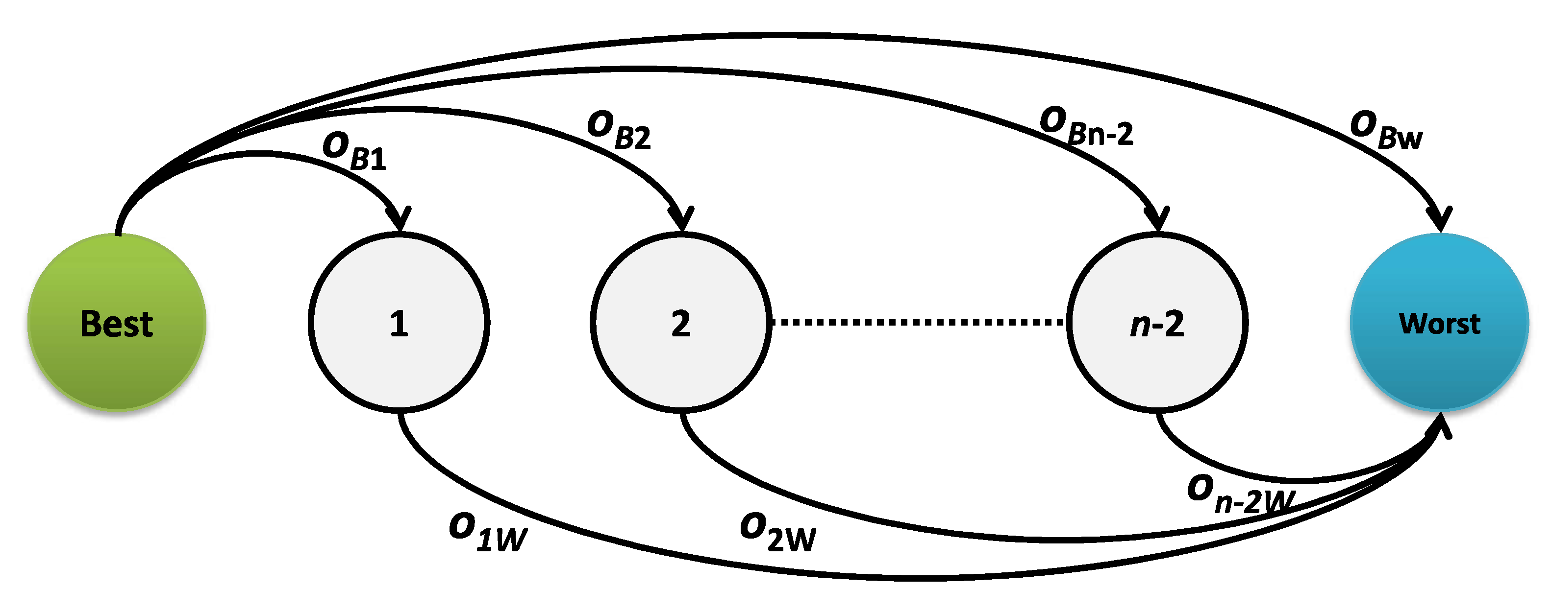
Step 3. All experts compare the best criterion ($C_B$) to all other criteria in pairs, yielding the best-to-others ($O_B^{E_k}$) vector depicted in Equation (7), as follows:

$$\begin{array}{cc}\hfill & o_B^{E_k}=(o_{B1}^{E_k},o_{B2}^{E_k},o_{B3}^{E_k},\dots ,o_{Bn}^{E_k})\forall k=1,2,\dots m.\hfill \end{array}$$

(7)

where $o_{Bj}^{E_k}\ge 1$, $j=1,2,\dots ,n$ reflects the level of preference for the best criterion $C_B$ over all other criteria $C_j$, $j\ne B$, given by the decision maker $E_k;k=1,2,\dots ,m$.

The pairwise comparison is presented in Figure 1.

Step 4. The others-to-worst ($O_W^{E_k}$) vector representing the pairwise comparison of preferences for each criterion and the least desirable criterion ($C_W$) for a group of experts is given in Equation (8) as:

$$\begin{array}{cc}\hfill & O_W^{E_k}={(o_{1W}^{E_k},o_{2W}^{E_k},o_{3W}^{E_k},\dots ,o_{nW}^{E_k})}^T\hfill \end{array}$$

(8)

where $o_{jW}^{E_k}\ge 1,j=1,2,\dots ,n,j\ne W$ shows how much the decision maker $E_k;k=1,2,\dots ,m$ prefers one criterion over another (in this case, the worst criterion $C_W$ over other criteria $C_j$).

Step 5. Combine all experts’ pairwise comparison values for the most important criterion $C_B$ over all other criteria $C_j,j=1,2,\cdots ,n$ when making decisions in groups using a multichoice approach, i.e., MCBWM. Then, the best-to-others ($O_B$) vector consists of experts’ comparison values as choices, as shown in Equation (9) as:

$$\begin{array}{cc}\hfill & O_B=\left(o_{B1},o_{B2},o_{B3},\dots ,o_{Bn}\right)\hfill \end{array}$$

(9)

where $o_{Bj}=\{o_{Bj}^{E_1},o_{Bj}^{E_2},o_{Bj}^{E_3},\dots ,o_{Bj}^{E_m}\}$. Furthermore, $o_{Bj}=\{o_{Bj}^1,o_{Bj}^2,\dots ,o_{Bj}^l\}\forall l=1,2,\dots ,9$ consists of all of the many choices for the comparison of the best criterion $C_B$ with the other criteria $C_j$, such that no two pairwise comparisons provided by the experts in the choice set are same.

Similarly, in Equation (10), the preferences for all criteria and the worst criterion are compared pairwise, and the results are presented in the others-to-worst ($O_W$) vector as follows:

$$\begin{array}{cc}\hfill & O_W={\left(o_{1W},o_{2W},o_{3W},\dots ,o_{nW}\right)}^T\hfill \end{array}$$

(10)

where $o_{jW}=\{o_{jW}^{E_1},o_{jW}^{E_2},o_{jW}^{E_3},\dots ,o_{jW}^{E_m}\}$. Furthermore, $o_{jW}=\{o_{jW}^1,o_{jW}^2,\dots ,o_{jW}^l\}\forall l=1,2,\dots ,9$ represents the collection of multichoice preference regarding the other criterion $C_j$ with the worst criterion $C_W$, such that no two pairwise comparisons provided by the experts in the choice set are equal. Therefore, the multichoice pairwise comparison matrix O is as follows:

$$\begin{array}{c}\hfill O=\left[\begin{array}{cccccccc}-& -& \cdots & -& \cdots & \{o_{1W}^1,o_{1W}^2,\cdots ,o_{1W}^l\}& \cdots & -\\ -& -& \cdots & -& \cdots & \{o_{2W}^1,o_{2W}^2,\cdots ,o_{2W}^l\}& \cdots & \\ ⋮& ⋮& ⋮& -& ⋮& ⋮& ⋮& ⋮\\ \{o_{B1}^1,o_{B1}^2,\cdots ,o_{B1}^l\}& \{o_{B2}^1,o_{B2}^2,\cdots ,o_{B2}^l\}& \cdots & 1& \cdots & \{o_{BW}^1,o_{BW}^2,\cdots ,o_{BW}^l\}& ⋮& \{o_{Bn}^1,o_{Bn}^2,\cdots ,o_{Bn}^l\}\\ ⋮& ⋮& ⋮& -& ⋮& ⋮& ⋮& ⋮\\ ⋮& ⋮& ⋮& -& ⋮& 1& ⋮& ⋮\\ ⋮& ⋮& ⋮& -& ⋮& ⋮& ⋮& ⋮\\ -& -& \cdots & -& \cdots & \{o_{nW}^1,o_{nW}^2,\cdots ,o_{nW}^l\}& \cdots & -\end{array}\right]\end{array}$$

(11)

Step 6. Find the optimal weights ($W_1^{*},W_2^{*},\dots ,W_n^{*}$) to rank the criteria, similar to the MCBWM approach. The mathematical programming model can be easily formulated as the following Model 2:

$$\begin{array}{cc}\hfill & \mathbf{Model}\mathbf{2}\hfill \end{array}$$

$$\begin{array}{cc}\hfill & Min\xi \hfill \\ \hfill & \mathrm{subject}\mathrm{to}\hfill \end{array}$$

(12)

$$\begin{array}{cc}\hfill & |W_B-W_j\times \{o_{Bj}^1,o_{Bj}^2,\dots ,o_{Bj}^l\}|\le \xi ,\forall j,l\hfill \end{array}$$

(13)

$$\begin{array}{cc}\hfill & |W_j-W_W\times \{o_{jW}^1,o_{jW}^2,\dots ,o_{jW}^l\}|\le \xi ,\forall j,l\hfill \end{array}$$

(14)

$$\begin{array}{cc}\hfill & \xi \ge 0,\sum W_j=1,W_j\ge 0,j=1,2,\cdots ,n\hfill \end{array}$$

(15)

where, $o_{Bj}=\{o_{Bj}^1,o_{Bj}^2,\cdots ,o_{Bj}^l\}$, and $o_{jW}=\{o_{jW}^1,o_{jW}^2,o_{jW}^3,\cdots ,o_{jW}^l\},\forall l=1,2,\cdots ,9$.

Step 7. Applying the Lagrange interpolating polynomial approach, we handle the multiple choices present in the constraints of Equations () and () and choose the option that will be responsible for minimizing the inconsistency.

Let $(0,1,2,\dots ,l-1)$ be the range of values for the node points represented by $z^{Bj}$ and $z^{jW}$ with respect to $o_{Bj}$ and $o_{jW}$. Thus, $\left\{o_{Bj}^1,o_{Bj}^2,o_{Bj}^3,\dots ,o_{Bj}^l\right\}$ and $\left\{o_{jW}^1,o_{jW}^2,o_{jW}^3,\dots ,o_{jW}^l\right\}$ are the associated functional values of the interpolating polynomial at l different node points. The node points and their functional values used to generate the polynomials for the constraints are shown in

Table 2. Node points and their functional values.

Polynomial	Description
$P_{l-1}\left(z^{Bj}\right)$	$z^{Bj}$	0	1	2	…	$l-1$
	$f\left(z^{Bj}\right)$	$o_{Bj}^1$	$o_{Bj}^2$	$o_{Bj}^3$	…	$o_{Bj}^l$
$P_{l-1}\left(z^{jW}\right)$	$z^{jW}$	0	1	2	…	$l-1$
	$f\left(z^{jW}\right)$	$o_{jW}^1$	$o_{jW}^2$	$o_{jW}^3$	…	$o_{jW}^l$

. The Lagrange interpolation formula for the $j^{th}$ criterion is used to build interpolating polynomials $P_{l-1}\left(z^{Bj}\right)$ and $P_{l-1}\left(z^{jW}\right)$ of degree $(l-1)$, whenever a multichoice parameter is used in the constraint function in Equations () and (), as shown below:

$$\begin{array}{cc}\hfill P_{l-1}\left(z^{Bj}\right)=& \frac{(z^{Bj}-1)(z^{Bj}-2)\dots (z^{Bj}-l+1)}{{(-1)}^{l-1}(l-1)!}{o}_{Bj}^1+\frac{z^{Bj}(z^{Bj}-2)\dots (z^{Bj}-l+1)}{{(-1)}^{l-2}(l-2)!}{o}_{Bj}^2\hfill \\ \hfill & +\frac{z^{Bj}(z^{Bj}-1)(z^{Bj}-3)\dots (z^{Bj}-l+1)}{{(-1)}^{l-3}(l-3)!2!}{o}_{Bj}^3\hfill \\ \hfill & +\cdots +\frac{z^{Bj}(z^{Bj}-1)(z^{Bj}-2)\dots (z^{Bj}-l+2)}{(l-1)!}{o}_{Bj}^l\forall j,l\hfill \end{array}$$

(16)

$$\begin{array}{cc}\hfill P_{l-1}\left(z^{jW}\right)=& \frac{(z^{jW}-1)(z^{jW}-2)\dots (z^{jW}-l+1)}{{(-1)}^{l-1}(l-1)!}{o}_{jW}^1+\frac{z^{jW}(z^{jW}-2)\dots (z^{jW}-l+1)}{{(-1)}^{l-2}(l-2)!}{o}_{jW}^2\hfill \\ \hfill & +\frac{z^{ijW}(z^{jW}-1)(z^{jW}-3)\dots (z^{jW}-l+1)}{{(-1)}^{l-3}(l-3)!2!}{o}_{jW}^3\hfill \\ \hfill & +\cdots +\frac{z^{jW}(z^{jW}-1)(z^{jW}-2)\dots (z^{jW}-l+2)}{(l-1)!}{o}_{jW}^l\forall j,l\hfill \end{array}$$

(17)

The resulting MCBWM optimization model is as follows:

$$\begin{array}{cc}\hfill & \mathbf{Model}\mathbf{3}\hfill \end{array}$$

$$\begin{array}{cc}\hfill & Min\xi \hfill \\ \hfill & \mathrm{subject}\mathrm{to}\hfill \end{array}$$

(18)

$$\begin{array}{cc}\hfill & W_B-W_j\times P_{l-1}\left(z^{Bj}\right)\le \xi ,\forall j\hfill \end{array}$$

(19)

$$\begin{array}{cc}\hfill & W_B-W_j\times P_{l-1}\left(z^{Bj}\right)\ge -\xi ,\forall j\hfill \end{array}$$

(20)

$$\begin{array}{cc}\hfill & W_j-W_W\times P_{l-1}\left(z^{jW}\right)\le \xi ,\forall j\hfill \end{array}$$

(21)

$$\begin{array}{cc}\hfill & W_j-W_W\times P_{l-1}\left(z^{jW}\right)\ge -\xi ,\forall j\hfill \end{array}$$

(22)

$$\begin{array}{cc}\hfill & \sum W_j=1,\hfill \end{array}$$

(23)

$$\begin{array}{cc}\hfill & W_j\ge 0,\forall j\hfill \end{array}$$

(24)

$$\begin{array}{cc}\hfill & \xi \ge 0\hfill \end{array}$$

(25)

$$\begin{array}{cc}\hfill & z^{Bj}=0,1,2,\dots ,(l-1)\forall j=1,2,3,\dots ,n\hfill \end{array}$$

(26)

$$\begin{array}{cc}\hfill & z^{jW}=0,1,2,\dots ,(l-1)\forall j=1,2,3,\dots ,n\hfill \end{array}$$

(27)

The decision variables, i.e., the weight of the criteria $W_j$, $z^{Bj}$, and $z^{jW};\forall j=1,2,\dots ,n$, and the multichoice programming problem (MCPP), as given above, can be solved.

The ideal weights and the best option are determined after the model is solved. The consistency ratio (CR) [12], which was used to assess the validity of the pairwise comparisons, is defined as follows:

$$\begin{array}{c}\hfill ConsistencyRatio=\frac{{\xi }^{*}}{ConsistencyIndex}\end{array}$$

(28)

where consistency index (CI) is a fixed value [12] and ${\xi }^{*}$ is the ideal objective value of model 3. After solving the mathematical model, $o_{BW}$ is used to determine the CI values. The CI is taken into consideration for $o_{BW}=o_{BW}^2$ if, for instance, $o_{BW}=\{o_{BW}^1,o_{BW}^2\}$, at the beginning and the node point $Z^{BW}=1$ is obtained after solving the model. In a similar manner, CI is taken into account for the value of $o_{BW}=o_{BW}^1$ if the node point obtained is $Z^{BW}=0$. The results are entirely consistent if CR is zero, and the consistency declines as CR rises. Additionally, the step-by-step process is shown in Figure 2.

4. Experimental Studies

Two numerical examples and one case study were selected to validate the MCBWM approach for group decision making. The two numerical examples and the first case study were taken from [36]. The data were further simulated to fit the multichoice assumption of the proposed approach.

4.1. Example 1

In this example, two DMs provided responses for four criteria. The first and third criteria were considered the best and worst, respectively. The pairwise comparison of the best and worst criterion with other criteria is given in

Table 3. Pairwise comparisons data for Example 1.

	${\mathit{o}}_{12}$	${\mathit{o}}_{13}$	${\mathit{o}}_{14}$	${\mathit{o}}_{23}$	${\mathit{o}}_{43}$
$DM1$	2	{8, 9}	3	4	2
$DM2$	2	8	{2, 3}	4	2
Multichoice	2	{8, 9}	{2, 3}	4	2

. The response from DM 1 for $o_{13}$ is considered a multichoice parameter with two values, 9 and 8. Additionally, for DM 2, the response $o_{14}=\{3,2\}$. The goal was that, out of all the pairwise comparison options given by DM 1 and 2, the best option or pairwise comparison should be chosen. In Table 3, the last row is the multichoice row, which presents all of the responses of DMs as choices. The MCGBWM model was formulated and solved using the proposed approach.

We considered the multichoice row in Table 3 as the responses of the DMs. The modeling of the proposed approach using mathematical programming was formulated and is presented below from (29)–(36).

$$\begin{array}{cc}\hfill & Min\xi \hfill \\ \hfill & \mathrm{subject}\mathrm{to}\hfill \end{array}$$

(29)

$$\begin{array}{cc}\hfill & W_1-W_2\times 2\le \xi ,W_1-W_2\times 2\ge -\xi \forall j\hfill \end{array}$$

(30)

$$\begin{array}{cc}\hfill & W_1-W_3\times (z^{13}+8)\le \xi ,W_1-W_3\times (z^{13}+8)\ge -\xi \forall j\hfill \end{array}$$

(31)

$$\begin{array}{cc}\hfill & W_1-W_4\times (z^{14}+2)\le \xi ,W_1-W_4\times (z^{14}+2)\ge -\xi \forall j\hfill \end{array}$$

(32)

$$\begin{array}{cc}\hfill & W_2-W_3\times 4\le \xi ,W_2-W_3\times 4\ge -\xi \forall j\hfill \end{array}$$

(33)

$$\begin{array}{cc}\hfill & W_4-W_3\times 2\le \xi ,W_4-W_3\times 2\ge -\xi \forall j\hfill \end{array}$$

(34)

$$\begin{array}{cc}\hfill & \sum W_j=1,W_j\ge 0,\forall j,\xi \ge 0\hfill \end{array}$$

(35)

$$\begin{array}{cc}\hfill & z^{13}=0,1,z^{14}=0,1\hfill \end{array}$$

(36)

Solving the proposed model by considering the multiple choices for Example 1, the optimal value of ${\xi }^{*}$ = 0.0266657; $z^{13}=1$, i.e., $o_{13}=8$; and $z^{14}=0$, i.e., $o_{14}=3$. The choice of $o_{BW}$, i.e., $o_{13}$ is equal to 8. So, CI=4.47 and, hence, CR=0.00059. This implies that the solution is highly consistent. The weight values and rank order of the criteria are provided in

Table 4. Optimal weights and CR of criteria for Example 1.

Methods	${\mathit{W}}_1$	${\mathit{W}}_2$	${\mathit{W}}_3$	${\mathit{W}}_4$	CR
Safarzadeh et al. [36] Model-1	0.528	0.222	0.065	0.185	0.096
Safarzadeh et al. [36] Model-2	0.512	0.246	0.063	0.179	0.096
Proposed approach	0.5067	0.2667	0.0667	0.16	0.0266657

. The optimal weights and CR of the criteria are presented in Figure 3.

In Table 4, we can see that the orders of the criteria obtained from the proposed model and using the approach of Safarzadeh et al. [36] are the same, i.e., $C_1>C_2>C_4>C_3$. There is a difference in the weights of the criteria. The CR obtained by the proposed method is 0.00059, which is better than that by Safarzadeh et al. [36], i.e., 0.096. The smaller the value of CR, the better.

The optimal weights’ ordering and the CR of the criteria are presented in Figure 3.

4.2. Example 2

In this example, we considered three DMs with four criteria. The first and fourth criteria were assumed to be the best and worst criteria, respectively. The preference values for comparisons with multichoice parameters are depicted in

Table 5. Three DMs’ pairwise comparison data for Example 2.

	${\mathit{o}}_{12}$	${\mathit{o}}_{13}$	${\mathit{o}}_{14}$	${\mathit{o}}_{23}$	${\mathit{o}}_{43}$
$DM1$	2	9	(3, 4)	4	2
$DM2$	2	(8, 9)	4	4	2
$DM3$	2	8	4	(3, 4)	2
Multichoice	2	(8, 9)	(3, 4)	(3, 4)	2

.

In Table 5, the last row is the multichoice response sets with $o_{13}=\{8,9\}$, $o_{14}=\{3,4\}$, and $o_{23}=\{3,4\}$. The data provided in the last row were used for solving the model of Example 2. The formulated model is presented in Equations (37)–(44).

$$\begin{array}{cc}\hfill & Min\xi \hfill \\ \hfill & \mathrm{subject}\mathrm{to}\hfill \end{array}$$

(37)

$$\begin{array}{cc}\hfill & W_1-W_2\times 2\le \xi ,W_1-W_2\times 2\ge -\xi \forall j\hfill \end{array}$$

(38)

$$\begin{array}{cc}\hfill & W_1-W_3\times (z^{13}+8)\le \xi ,W_1-W_3\times (z^{13}+8)\ge -\xi \forall j\hfill \end{array}$$

(39)

$$\begin{array}{cc}\hfill & W_1-W_4\times (z^{14}+3)\le \xi ,W_1-W_4\times (z^{14}+3)\ge -\xi \forall j\hfill \end{array}$$

(40)

$$\begin{array}{cc}\hfill & W_2-W_3\times (z^{23}+3)\le \xi ,W_2-W_3\times (z^{23}+3)\ge -\xi \forall j\hfill \end{array}$$

(41)

$$\begin{array}{cc}\hfill & W_4-W_3\times 2\le \xi ,W_4-W_3\times 2\ge -\xi \forall j\hfill \end{array}$$

(42)

$$\begin{array}{cc}\hfill & \sum W_j=1,W_j\ge 0,\forall j,\xi \ge 0\hfill \end{array}$$

(43)

$$\begin{array}{cc}\hfill & z^{13}=0,1z^{14}=0,1z^{23}=0,1\hfill \end{array}$$

(44)

The optimal values ${\xi }^{*}$=0 and $z^{13}=1$, i.e., $o_{13}=9$; $z^{14}=1$, i.e., $o_{14}=4$; and $z^{23}=0$, i.e., $o_{23}=3$. The value of $o_{BW}=9$ as $z^{13}=1$. The corresponding CR becomes equal to 0. The weights and ranks of the criteria are provided in

Table 6. Optimal weights and CR of criteria for Example 2.

Methods	${\mathit{W}}_1$	${\mathit{W}}_2$	${\mathit{W}}_3$	${\mathit{W}}_4$	CR
Safarzadeh et al. [36] Model 1	0.553	0.226	0.066	0.155	0.040
Safarzadeh et al. [36] Model 2	0.551	0.227	0.065	0.157	0.045
Proposed approach	0.534	0.267	0.067	0.134	0

.

In Table 6, the orders of the ranks obtained from the proposed model and by the method of Safarzadeh et al. [36] for the criteria are the same, i.e., $C_1>C_2>C_4>C_3$. There is a slight difference in the criteria weights. The CR obtained using the developed approach is 0, which is far better than that of Safarzadeh et al. [36] approach, i.e., 0.040 and 0.045 for Models 1 and 2, respectively. The optimal weights, ordering, and CR of the criteria for Example 2 are presented in Figure 4.

4.3. Case Study

Ten decision makers in an actual case study [36] about a piping selection method were taken into consideration, with four categories: overall cost ($C_1$), security cost ($C_2$), social cost ($C_3$), and environmental cost ($C_4$). The best criterion was the total cost ($C_B$), whereas the worst criterion was the environmental cost ($C_W$).

In

Table 7. Case study.

	${\mathit{o}}_{12}$	${\mathit{o}}_{13}$	${\mathit{o}}_{14}$	${\mathit{o}}_{24}$	${\mathit{o}}_{34}$
$DM1$	{6, 7}	6	7	4	{2, 3}
$DM2$	7	7	{7, 9}	{4, 6}	5
$DM3$	7	{6, 7}	9	{8, 9}	8
$DM4$	{2, 3, 5}	4	{6, 7}	4	3
$DM5$	3	4	8	{3, 4, 5}	5
$DM6$	5	{6, 7}	7	5	{2, 3, 5}
$DM7$	9	{4, 6}	9	9	8
$DM8$	9	{7, 9}	9	{6, 8}	2
$DM9$	{8, 9}	9	9	{3, 4}	1
$DM10$	{7, 9}	9	9	{3, 5}	{1, 2, 3}
Multi-choice	{2, 3, 5, 6, 7, 8, 9}	{4, 6, 7, 9}	{6, 7, 8, 9}	{3, 4, 5, 6, 8, 9}	{1, 2, 3, 5, 8}

, the preference value information for the case study is provided. The multichoice data are also presented. Once we had the data in multichoice form, we applied the proposed multichoice method. The mathematical programming model is presented in Equations (45)–(57).

$$\begin{array}{cc}\hfill & Min\xi \hfill \\ \hfill & \mathrm{subject}\mathrm{to}\hfill \end{array}$$

(45)

$$\begin{array}{cc}\hfill & W_1-W_2\times \left(\frac{{\left(z^{12}\right)}^6}{144}-\frac{11{\left(z^{12}\right)}^5}{80}+\frac{151{\left(z^{12}\right)}^4}{144})-\frac{61{\left(z^{12}\right)}^3}{16}+\frac{58{\left(z^{12}\right)}^2}{9}-\frac{51z^{12}}{20}+2\right)\le \xi ,\forall j\hfill \end{array}$$

(46)

$$\begin{array}{cc}\hfill & W_1-W_2\times \left(\frac{{\left(z^{12}\right)}^6}{144}-\frac{11{\left(z^{12}\right)}^5}{80}+\frac{151{\left(z^{12}\right)}^4}{144})-\frac{61{\left(z^{12}\right)}^3}{16}+\frac{58{\left(z^{12}\right)}^2}{9}-\frac{51z^{12}}{20}+2\right)\ge -\xi ,\forall j\hfill \end{array}$$

(47)

$$\begin{array}{cc}\hfill & W_1-W_3\times \left(\frac{{\left(z^{13}\right)}^3)}{3}-\frac{3{\left(z^{13}\right)}^2}{2}+\frac{19z^{13}}{6}+4\right)\le \xi ,\forall j\hfill \end{array}$$

(48)

$$\begin{array}{cc}\hfill & W_1-W_3\times \left(\frac{{\left(z^{13}\right)}^3)}{3}-\frac{3{\left(z^{13}\right)}^2}{2}+\frac{19z^{13}}{6}+4\right)\ge -\xi ,\forall j\hfill \end{array}$$

(49)

$$\begin{array}{cc}\hfill & W_1-W_4\times (z^{14}+6)\le \xi ,\forall j\hfill \end{array}$$

(50)

$$\begin{array}{cc}\hfill & W_1-W_4\times (z^{14}+6)\ge -\xi ,\forall j\hfill \end{array}$$

(51)

$$\begin{array}{cc}\hfill & W_2-W_4\times \left(\frac{-{\left(z^{24}\right)}^5}{30}+\frac{3{\left(z^{24}\right)}^4}{8}-\frac{17{\left(z^{24}\right)}^3}{12}+\frac{17{\left(z^{24}\right)}^2}{8}-\frac{z^{24}}{20}+3\right)\le \xi ,\forall j\hfill \end{array}$$

(52)

$$\begin{array}{cc}\hfill & W_2-W_4\times \left(\frac{-{\left(z^{24}\right)}^5}{30}+\frac{3{\left(z^{24}\right)}^4}{8}-\frac{17{\left(z^{24}\right)}^3}{12}+\frac{17{\left(z^{24}\right)}^2}{8}-\frac{z^{24}}{20}+3\right)\ge -\xi ,\forall j\hfill \end{array}$$

(53)

$$\begin{array}{cc}\hfill & W_3-W_4\times \left(\frac{-{\left(z^{34}\right)}^4}{24}+\frac{5{\left(z^{34}\right)}^3}{12}-\frac{23{\left(z^{34}\right)}^2}{24}+\frac{19\left(z^{34}\right)}{12}+1\right)\le \xi ,\forall j\hfill \end{array}$$

(54)

$$\begin{array}{cc}\hfill & W_3-W_4\times \left(\frac{-{\left(z^{34}\right)}^4}{24}+\frac{5{\left(z^{34}\right)}^3}{12}-\frac{23{\left(z^{34}\right)}^2}{24}+\frac{19\left(z^{34}\right)}{12}+1\right)\ge -\xi ,\forall j\hfill \end{array}$$

(55)

$$\begin{array}{cc}\hfill & \sum W_j=1,W_j\ge 0,\forall j,\xi \ge 0\hfill \end{array}$$

(56)

$$\begin{array}{cc}\hfill & z^{12}=0,1,2,3,4,5,6,z^{13}=0,1,2,3,z^{14}=0,1,2,3,z^{24}=0,1,2,3,4,5,z^{34}=0,1,2,3,4\hfill \end{array}$$

(57)

Now solving the above model of the MCBWM, the results were obtained. The optimal value of ${\xi }^{*}$= 0 and $z^{12}=0$, i.e., $o_{12}=2$ $z^{13}=1$, i.e., $o_{13}=6$; $z^{14}=0$, i.e., $o_{14}=6$; $z^{24}=0$, i.e., $o_{24}=3$; and $z^{34}=0$,i.e., $o_{34}=1$. For the obtained choice of pairwise comparisons, the weight values are presented in

Table 8. Optimal weights, ordering, and CR of criteria for case study.

Methods	${\mathit{W}}_1$	${\mathit{W}}_2$	${\mathit{W}}_3$	${\mathit{W}}_4$	CR
Safarzadeh et al. [36] Model-1	0.718	0.111	0.096	0.075	0.169
Safarzadeh et al. [36] Model-2	0.649	0.146	0.138	0.067	0.183
Group-AHP [36]	0.677	0.192	0.079	0.053	0.090
Proposed approach	0.545	0.272	0.090	0.090	0

. In Table 8, we can see that the obtained order through the proposed model is the same as that obtained by Safarzadeh et al. [36] and group-AHP, as mentioned in [36], i.e., $C_1>C_2>C_3>C_4$. The CR value in the case of the proposed model is far better in comparison with that of the other approaches. The reason for this is the multichoice behavior of the model, which allows choosing that choice of pairwise comparison, which minimizes the inconsistency. The optimal weights, ordering, and CR of the criteria for the case study are presented in Figure 5.

5. Conclusions, Limitations, and Future Work

In the present study, we developed an approach for solving decision-making problems involving a group of experts. The proposed approach differs from existing models as it considers choices in pairwise comparisons. It provides freedom to experts to choose multiple responses to compare criteria. The developed model chooses the best responses collected from experts so that the inconsistency is minimized, and the optimal criteria weights are obtained. The idea of the proposed approach is an extension of the MCBWM [28] to group decision making. Hasan et al. [28] demonstrated the applicability of MCBWM in MCDM problems. In this paper, the step-wise procedure of the proposed approach was presented.

The multichoice approach changes the best to all and others to the worst vector to the vector for which inconsistency is minimized. The objective is to look for the choices with the least inconsistency. The advantage of the proposed approach is that it considers the pairwise comparison values from all experts in a choice set and chooses the one for which inconsistency is minimized. The proposed method considers the human perception and cognition of having the choice in their suggestions.

The proposed model was validated using three examples. In all examples, we observed that pairwise importance was compared with the freedom of choosing multiple pairwise comparisons, as choices are combined into one choice set. The developed model was formulated and solved for the ideal weights of the criteria. The results were presented through tables and figures. The results achieved utilizing the developed approach were compared with those of other existing approaches [36]. The weights of the criteria slightly differed without affecting the priority order of the criteria. For all examples, the obtained CR value was better than the CR of existing approaches. The proposed approach was validated by comparing the CR and the order of the criteria obtained. In the proposed method, the obtained CR was either equal to or less than that of the other considered methods, which makes it more or equally reliable. This shows the advantage of the proposed approach over other methods.

The proposed approach also has limitations. It lacks consensus, as in other BWM approaches. The best pairwise comparison value from a multichoice set, for which inconsistency is minimized, was considered in the proposed approach. This is a new way of reducing inconsistency in group decision making. This limitation can be overcome by incorporating concepts such as belief theory [47] and confidence levels [48]. Another limitation is that we did not consider the confidence level of the experts for the multichoice response values provided by them. The technicality of the proposed approach makes it difficult to implement. In a future study, these limitations can be rectified.

In the near future, we think that the proposed approach can be further extended by involving uncertainty using, for example, fuzzy theory [37], neutrosophic [48], fermatean [49], hesitant [50], probabilistic hesitant fuzzy [51], personalized individual semantics [52], confidence level [48], etc. We did not consider any kind of consensus but considered experts’ decisions as choices; so, in the future, we can extend the proposed approach by incorporating the consensus of the decision makers [48,53,54] along with the multichoice set. The proposed model can also be implemented for some modern problems; see [55,56,57].

References

- Saaty, T.L. Decision making—The analytic hierarchy and network processes (AHP/ANP). J. Syst. Sci. Syst. Eng. 2004, 13, 1–35. [Google Scholar] [CrossRef]
- Zeleny, M. Multiple Criteria Decision Making Kyoto 1975; Springer Science & Business Media: Berlin/Heidelberg, Germany, 2012; Volume 123. [Google Scholar]
- Zavadskas, E.K.; Turskis, Z. Multiple criteria decision making (MCDM) methods in economics: An overview. Technol. Econ. Dev. Econ. 2011, 17, 397–427. [Google Scholar] [CrossRef] [Green Version]
- Wallenius, J.; Dyer, J.S.; Fishburn, P.C.; Steuer, R.E.; Zionts, S.; Deb, K. Multiple criteria decision making, multiattribute utility theory: Recent accomplishments and what lies ahead. Manag. Sci. 2008, 54, 1336–1349. [Google Scholar] [CrossRef] [Green Version]
- Ahmad, N.; Hasan, M.G.; Barbhuiya, R.K. Identification and prioritization of strategies to tackle COVID-19 outbreak: A group-BWM based MCDM approach. Appl. Soft Comput. 2021, 111, 107642. [Google Scholar] [CrossRef]
- Shameem, M.; Khan, A.A.; Hasan, M.G.; Akbar, M.A. Analytic hierarchy process based prioritisation and taxonomy of success factors for scaling agile methods in global software development. IET Softw. 2020, 14, 389–401. [Google Scholar] [CrossRef]
- Saaty, T.L.; Ergu, D. When is a decision-making method trustworthy? Criteria for evaluating multicriteria decision-making methods. Int. J. Inf. Technol. Decis. Mak. 2015, 14, 1171–1187. [Google Scholar] [CrossRef]
- Ayan, B.; Abacıoğlu, S.; Basilio, M.P. A Comprehensive Review of the Novel Weighting Methods for Multi-Criteria Decision-Making. Information 2023, 14, 285. [Google Scholar] [CrossRef]
- Do, D.T.; Nguyen, N.T. Applying Cocoso, Mabac, Mairca, Eamr, Topsis and weight determination methods for multicriteria decision making in hole turning process. Stroj. Čas.-J. Mech. Eng. 2022, 72, 15–40. [Google Scholar]
- Basílio, M.P.; Pereira, V.; Costa, H.G.; Santos, M.; Ghosh, A. A systematic review of the applications of multicriteria decision aid methods (1977–2022). Electronics 2022, 11, 1720. [Google Scholar] [CrossRef]
- Sałabun, W.; Wątróbski, J.; Shekhovtsov, A. Are mcda methods benchmarkable? a comparative study of topsis, vikor, copras, and promethee ii methods. Symmetry 2020, 12, 1549. [Google Scholar] [CrossRef]
- Rezaei, J. Best-worst multicriteria decision-making method. Omega 2015, 53, 49–57. [Google Scholar] [CrossRef]
- Mi, X.; Tang, M.; Liao, H.; Shen, W.; Lev, B. The state-of-the-art survey on integrations and applications of the best worst method in decision making: Why, what, what for and what’s next? Omega 2019, 87, 205–225. [Google Scholar] [CrossRef]
- Rezaei, J.; Wang, J.; Tavasszy, L. Linking supplier development to supplier segmentation using Best Worst Method. Expert Syst. Appl. 2015, 42, 9152–9164. [Google Scholar] [CrossRef]
- Liu, P.; Zhu, B.; Wang, P. A weighting model based on best–worst method and its application for environmental performance evaluation. Appl. Soft Comput. 2021, 103, 107168. [Google Scholar] [CrossRef]
- Dong, J.; Wan, S.; Chen, S.M. Fuzzy best–worst method based on triangular fuzzy numbers for multicriteria decision-making. Inf. Sci. 2021, 547, 1080–1104. [Google Scholar] [CrossRef]
- Qu, S.; Xu, Y.; Wu, Z.; Xu, Z.; Ji, Y.; Qu, D.; Han, Y. An interval-valued best–worst method with normal distribution for multicriteria decision-making. Arab. J. Sci. Eng. 2021, 46, 1771–1785. [Google Scholar] [CrossRef]
- Li, J.; Niu, L.l.; Chen, Q.; Wang, Z.X. Approaches for multicriteria decision-making based on the hesitant fuzzy best–worst method. Complex Intell. Syst. 2021, 7, 2617–2634. [Google Scholar] [CrossRef]
- Torkayesh, A.E.; Malmir, B.; Asadabadi, M.R. Sustainable waste disposal technology selection: The stratified best–worst multicriteria decision-making method. Waste Manag. 2021, 122, 100–112. [Google Scholar] [CrossRef]
- Ahmad, N.; Hasan, M.G. Self-adaptive query-broadcast in wireless ad-hoc networks using fuzzy best worst method. Wirel. Netw. 2021, 27, 765–780. [Google Scholar] [CrossRef]
- Ghaffar, A.R.A.; Nadeem, M.R.; Hasan, M.G. Cost-Benefit Analysis of Shale Development in India: A Best-Worst Method based MCDM approach. J. King Saud-Univ.-Sci. 2021, 33, 101591. [Google Scholar] [CrossRef]
- Singh, M.; Rathi, R.; Garza-Reyes, J.A. Analysis and prioritization of Lean Six Sigma enablers with environmental facets using best worst method: A case of Indian MSMEs. J. Clean. Prod. 2021, 279, 123592. [Google Scholar] [CrossRef]
- Xu, Y.; Zhu, X.; Wen, X.; Herrera-Viedma, E. Fuzzy best–worst method and its application in initial water rights allocation. Appl. Soft Comput. 2021, 101, 107007. [Google Scholar] [CrossRef]
- Sen, M.K.; Dutta, S.; Kabir, G. Development of flood resilience framework for housing infrastructure system: Integration of best–worst method with evidence theory. J. Clean. Prod. 2021, 290, 125197. [Google Scholar] [CrossRef]
- Mostafaeipour, A.; Alvandimanesh, M.; Najafi, F.; Issakhov, A. Identifying challenges and barriers for development of solar energy by using fuzzy best–worst method: A case study. Energy 2021, 226, 120355. [Google Scholar] [CrossRef]
- Hsu, H.Y.; Hwang, M.H.; Tsou, P.H. Applications of BWM and GRA for Evaluating the Risk of Picking and Material-Handling Accidents in Warehouse Facilities. Appl. Sci. 2023, 13, 1263. [Google Scholar] [CrossRef]
- Zhao, G.; Kang, T.; Guo, J.; Zhang, R.; Li, L. Gray relational analysis optimization for coalbed methane blocks in complex conditions based on a best worst and entropy method. Appl. Sci. 2019, 9, 5033. [Google Scholar] [CrossRef] [Green Version]
- Hasan, M.G.; Ashraf, Z.; Khan, M.F. Multi-choice best–worst multicriteria decision-making method and its applications. Int. J. Intell. Syst. 2022, 37, 1129–1156. [Google Scholar] [CrossRef]
- Biswal, M.; Acharya, S. Solving multichoice linear programming problems by interpolating polynomials. Math. Comput. Model. 2011, 54, 1405–1412. [Google Scholar] [CrossRef]
- Quddoos, A.; ull Hasan, M.G.; Khalid, M.M. Multi-choice stochastic transportation problem involving general form of distributions. SpringerPlus 2014, 3, 565. [Google Scholar] [CrossRef] [Green Version]
- Singh, S.; Sonia. Multi-choice programming: An overview of theories and applications. Optimization 2017, 66, 1713–1738. [Google Scholar] [CrossRef]
- Mou, Q.; Xu, Z.; Liao, H. An intuitionistic fuzzy multiplicative best–worst method for multicriteria group decision making. Inf. Sci. 2016, 374, 224–239. [Google Scholar] [CrossRef]
- You, X.; Chen, T.; Yang, Q. Approach to multicriteria group decision-making problems based on the best–worst-method and electre method. Symmetry 2016, 8, 95. [Google Scholar] [CrossRef] [Green Version]
- Hafezalkotob, A.; Hafezalkotob, A. A novel approach for combination of individual and group decisions based on fuzzy best–worst method. Appl. Soft Comput. 2017, 59, 316–325. [Google Scholar] [CrossRef]
- Mohammadi, M.; Rezaei, J. Bayesian best–worst method: A probabilistic group decision making model. Omega 2019, 96, 102075. [Google Scholar] [CrossRef]
- Safarzadeh, S.; Khansefid, S.; Rasti-Barzoki, M. A group multicriteria decision-making based on best–worst method. Comput. Ind. Eng. 2018, 126, 111–121. [Google Scholar] [CrossRef]
- Guo, S.; Qi, Z. A Fuzzy Best-Worst Multi-Criteria Group Decision-Making Method. IEEE Access 2021, 9, 118941–118952. [Google Scholar] [CrossRef]
- Haseli, G.; Sheikh, R.; Wang, J.; Tomaskova, H.; Tirkolaee, E.B. A novel approach for group decision making based on the best–worst method (G-bwm): Application to supply chain management. Mathematics 2021, 9, 1881. [Google Scholar] [CrossRef]
- Emamat, M.S.M.M.; Amiri, M.; Mehregan, M.R.; Taghavifard, M.T. A novel hybrid simplified group BWM and multicriteria sorting approach for stock portfolio selection. Expert Syst. Appl. 2023, 215, 119332. [Google Scholar] [CrossRef]
- Gupta, H.; Kharub, M.; Shreshth, K.; Kumar, A.; Huisingh, D.; Kumar, A. Evaluation of strategies to manage risks in smart, sustainable agri-logistics sector: A Bayesian-based group decision-making approach. Bus. Strategy Environ. 2023. [Google Scholar] [CrossRef]
- Tavana, M.; Mina, H.; Santos-Arteaga, F.J. A general Best-Worst method considering interdependency with application to innovation and technology assessment at NASA. J. Bus. Res. 2023, 154, 113272. [Google Scholar] [CrossRef]
- Zhang, H.; Wang, X.; Xu, W.; Dong, Y. From numerical to heterogeneous linguistic best–worst method: Impacts of personalized individual semantics on consistency and consensus. Eng. Appl. Artif. Intell. 2023, 117, 105495. [Google Scholar] [CrossRef]
- Ma, X.; Qin, J.; Martínez, L.; Pedrycz, W. A linguistic information granulation model based on best–worst method in decision making problems. Inf. Fusion 2023, 89, 210–227. [Google Scholar] [CrossRef]
- Qin, J.; Ma, X.; Liang, Y. Building a consensus for the best–worst method in group decision-making with an optimal allocation of information granularity. Inf. Sci. 2023, 619, 630–653. [Google Scholar] [CrossRef]
- Özay, B.; Orhan, O. Flood susceptibility mapping by best–worst and logistic regression methods in Mersin, Turkey. Environ. Sci. Pollut. Res. 2023, 30, 45151–45170. [Google Scholar] [CrossRef] [PubMed]
- Nayeri, S.; Sazvar, Z.; Heydari, J. Towards a responsive supply chain based on the industry 5.0 dimensions: A novel decision-making method. Expert Syst. Appl. 2023, 213, 119267. [Google Scholar] [CrossRef]
- Liang, F.; Brunelli, M.; Septian, K.; Rezaei, J. Belief-Based Best Worst Method. Int. J. Inf. Technol. Decis. Mak. 2021, 20, 287–320. [Google Scholar] [CrossRef]
- Vafadarnikjoo, A.; Tavana, M.; Botelho, T.; Chalvatzis, K. A neutrosophic enhanced best–worst method for considering decision-makers’ confidence in the best and worst criteria. Ann. Oper. Res. 2020, 289, 391–418. [Google Scholar] [CrossRef]
- Simic, V.; Gokasar, I.; Deveci, M.; Isik, M. Fermatean fuzzy group decision-making based CODAS approach for taxation of public transit investments. IEEE Trans. Eng. Manag. 2021. [Google Scholar] [CrossRef]
- Liu, X.; Wang, Z.; Zhang, S.; Garg, H. Novel correlation coefficient between hesitant fuzzy sets with application to medical diagnosis. Expert Syst. Appl. 2021, 183, 115393. [Google Scholar] [CrossRef]
- Liu, X.; Wang, Z.; Zhang, S.; Garg, H. An approach to probabilistic hesitant fuzzy risky multiattribute decision making with unknown probability information. Int. J. Intell. Syst. 2021, 36, 5714–5740. [Google Scholar] [CrossRef]
- Zhang, H.; Dong, Y.; Xiao, J.; Chiclana, F.; Herrera-Viedma, E. Personalized individual semantics-based approach for linguistic failure modes and effects analysis with incomplete preference information. IISE Trans. 2020, 52, 1275–1296. [Google Scholar] [CrossRef] [Green Version]
- Zhang, H.; Wang, F.; Dong, Y.; Chiclana, F.; Herrera-Viedma, E. Social Trust Driven Consensus Reaching Model with a Minimum Adjustment Feedback Mechanism Considering Assessments-Modifications Willingness. IEEE Trans. Fuzzy Syst. 2021, 30, 2019–2031. [Google Scholar] [CrossRef]
- Xiao, J.; Wang, X.; Zhang, H. Exploring the ordinal classifications of failure modes in the reliability management: An optimization-based consensus model with bounded confidences. Group Decis. Negot. 2022, 31, 49–80. [Google Scholar] [CrossRef]
- Maddeh, M.; Al-Otaibi, S.; Alyahya, S.; Hajjej, F.; Ayouni, S. A Comprehensive MCDM-Based Approach for Object-Oriented Metrics Selection Problems. Appl. Sci. 2023, 13, 3411. [Google Scholar] [CrossRef]
- Nallakaruppan, M.K.; Johri, I.; Somayaji, S.; Bhatia, S.; Malibari, A.A.; Alabdali, A.M. Secured MCDM Model for Crowdsource Business Intelligence. Appl. Sci. 2023, 13, 1511. [Google Scholar] [CrossRef]
- Sgarbossa, F.; Peron, M.; Fragapane, G. Cloud material handling systems: Conceptual model and cloud-based scheduling of handling activities. In Scheduling in Industry 4.0 and Cloud Manufacturing; Springer: Berlin/Heidelberg, Germany, 2020; pp. 87–101. [Google Scholar]
Figure 1.
Pairwise comparison.
Figure 2.
Steps of proposed approach.
Figure 3.
Optimal weights, ordering, and CR of criteria for Example 1.
Figure 4.
Optimal weights, ordering, and CR of criteria for Example 2.
Figure 5.
Optimal weights, ordering, and CR of criteria for case study.