Two-Stage Deep Learning Method for Breast Cancer Detection Using High-Resolution Mammogram Images

Abstract

Breast cancer screening and detection using high-resolution mammographic images have always been a difficult task in computer vision due to the presence of very small yet clinically significant abnormal growths in breast masses. The size difference between such masses and the overall mammogram image as well as difficulty in distinguishing intra-class features of the Breast Imaging Reporting and Database System (BI-RADS) categories creates challenges for accurate diagnosis. To obtain near-optimal results, object detection models should be improved by directly focusing on breast cancer detection. In this work, we propose a new two-stage deep learning method. In the first stage, the breast area is extracted from the mammogram and small square patches are generated to narrow down the region of interest (RoI). In the second stage, breast masses are detected and classified into BI-RADS categories. To improve the classification accuracy for intra-classes, we design an effective tumor classification model and combine its results with the detection model’s classification scores. Experiments conducted on the newly collected high-resolution mammography dataset demonstrate our two-stage method outperforms the original Faster R-CNN model by improving mean average precision (mAP) from 0.85 to 0.94. In addition, comparisons with existing works on a popular INbreast dataset validate the performance of our two-stage model.

1. Introduction

Accurate and early detection of breast cancer is substantial to fight against the second highest cause of mortality in women. According to the World Health Organization (WHO), new cases of breast cancer were diagnosed in over 2 million women globally in 2020 and are predicted to increase by 70% in the next 20 years [1]. Early detection of breast cancer potentially doubles the survival rate. Breast cancer diagnosis includes correctly identifying each stage and classifying detected breast tumors and abnormalities into proper categories. In order to assist radiologists and oncologists in diagnosing breast cancer in a fast and reliable manner, many computer-aided diagnosis (CAD) systems have been developed over the last two decades [2]. Unfortunately, earlier CAD systems did not produce significant improvements in day-to-day breast cancer diagnosis in clinical use [3,4]. After the ‘boom’ of deep learning (DL), DL-based CAD systems and other computer vision and object recognition methods brought success to many areas of medicine, from day-to-day healthcare practices to comprehensive medical applications [5,6,7,8]. Currently, there are many DL-based CAD systems that can be used to assist radiologists in breast cancer screening, monitoring, and diagnosis. Recent studies [9,10] suggest that DL-based object detection and segmentation models, in particular, can potentially perform as well as radiologists in standalone mode by producing accurate and reliable results. However, before directly applying such models to diagnose breast cancer, especially when using high-resolution digital mammography images, certain challenges and issues need to be addressed carefully.

One of the main challenges in accurately detecting breast masses (mass and tumor are used interchangeably) from high-resolution mammography images is that the ratio of some breast masses to the overall image size is too small. For instance, some clinically significant abnormal growth or even potentially cancerous tumors may lie within 100 × 100-pixel regions [10], whereas the size of digital mammography images is usually 5900 × 4700 pixels. Furthermore, some breast masses can still be greater in size but have very low contrast which can be overlooked when examining the full-sized high-resolution mammograms. Some prior work [11,12,13] addressed this issue by using manually annotated lesions to narrow down the potential region of interest (RoI) so that deep learning models can focus only on that RoI. However, manually annotating RoI is laborious and ultimately restricts to having fully automated real-world applications due to the absence of such annotated RoI for in-the-wild data. Shen et al. [10] trained a model on a Curated Breast Imaging Subset of Digital Database for Screening Mammography (CBIS-DDSM) database that contains annotated RoI and transferred the model RoI extraction layers for the INbreast dataset [14]. However, this approach still requires manually annotated RoIs for initial network training. Other studies [5,6,15] attempted to train deep convolutional neural networks (CNN) using the whole mammogram images. Unfortunately, due to the input size restrictions and pooling layers (i.e., downsampling), even state-of-the-art object detection models miss some of the significant lesions or micro-calcifications. Singh et al. [15] used a Single-shot detector (SSD) [16] object detection model for the whole mammogram to obtain RoIs for further tumor shape classification. However, the accuracy of the classification is based on the premise that SSD is able to detect all tumors, which in general, is not true. Considering these issues, appropriate automatic RoI extraction methods should be exploited.

Another common issue in breast cancer diagnosis is that most of the existing DL-based models classify detected tumors/abnormalities into benign and malignant categories [10,15,17,18,19]. Although this is the main motivation behind breast cancer diagnosis, such binary classification-based models cannot directly assist radiologists in breast cancer screening and reporting. In the majority of real-world scenarios and applications, the Breast Imaging Reporting and Database System (BI-RADS) [20,21,22] score, which is a standard scoring system, is used by radiologists to report mammogram results. BI-RADS scores are classified into incomplete assessment (category 0) and complete assessment (categories 1, 2, 3, 4, 5, 6). The description of each category is presented in

Table 1. Description of BI-RADS categories.

BI-RADS Catogory	Assessment	Suspicion of Malignancy	Clinical Recommendation
0	Assessment incomplete	-	Need to review prior studies or complete additional screening
1	Negative	≈0	Continue routine screening
2	Benign cysts or other findings	≈0	Continue routine screening
3	Probably benign finding	<2%	Short-term follow-up screening
4	Suspicious abnormality	≥2% to <10% (4a) ≥10% to <50% (4b) ≥50% to <95% (4c)	Perform needle biopsy
5	Highly suspicion of malignancy	≥95%	Biopsy and treatment
6	Known biopsy-proven malignancy	100%	Pending/ongoing treatment should be completed, surgical excision if appropriate

. The classification of the corresponding BI-RADS score recommends specific clinical screening routines which are important for appropriate patient treatment and follow-up screening. Moreover, BI-RADS scores provide a wide range of suspicion of malignancy and are considered more descriptive than classifying tumors into just two classes: benign and malignant. Therefore, it is important to build CAD systems according to the BI-RADS lexicon. Unfortunately, despite the presence of BI-RADS scores in the above-mentioned DDSM and INbreast databases, prior studies [10,15,17,18,19] classify the detected tumors into binary classes (e.g., BI-RADS 1, 2 as benign and BI-RADS 4, 5, 6 as malignant). In this study, we aim to propose a model according to the BI-RADS lexicon and improve classification specificity and sensitivity by thoroughly examining distinct intra-class features and attributes (e.g., BI-RADS 4c vs. 5, BI-RADS 4a vs. 4b), which is not the case for binary classification.

Finally, the lack of large open datasets of modern high-resolution digital mammograms containing labeled BI-RADS scores, annotated RoIs, bounding-box coordinates, and masks creates challenges in developing unified and robust CAD systems. To overcome this issue, prior studies [10,17,18] used pre-trained models and transferred the network knowledge to diagnose breast cancer in smaller datasets. For instance, Shams et al. [17] trained the original model on DDSM database of digitized film mammograms and, using transfer learning, fine-tuned the network parameters on INbreast [14] training data to build a classifier for INbreast data. In addition, as previously discussed, Shen et al. [10] also carried out similar experiments. In this study, we introduce our newly collected high-resolution mammograms dataset with accurately labeled BI-RADS scores.

In this paper, we propose a two-stage deep learning method for accurate breast cancer detection and classification. Stage 1 extracts ‘potential’ RoI patches from the original input data without the need for human labor, whereas stage 2 detects breast masses, improves bounding box regions, and classifies them into the BI-RADS categories. Numerous data pre-processing steps are introduced and a specifically-designed CNN-based tumor classification model is proposed to further improve the classification accuracy obtained from the detection model. The key contributions are as follows:

• We collected a new dataset of high-resolution mammography images and annotated them with BI-RADS lexicon, which provides a more reliable and a wider range of suspicion of malignancy;
• We propose a two-stage deep learning approach to significantly increase detection accuracy. To this extent, we introduce square patch generation, bounding-box mapping, and duplication removal algorithms to automatically extract RoIs from the input data, and map back the patch detections into the original image without human supervision and labor;
• We design a tumor classification model to improve the classification accuracy of breast tumors obtained by the object detection model. The output of the classification model is combined with the output scores of the object detection model’s classifier to get the final output.

2. Datasets

In this study, we use two datasets to conduct our experiments. The first dataset is collected and accurately labeled by senior radiologists with BI-RADS categories. We show the effectiveness of our two-stage methodology on this dataset. The second dataset is a publicly available INbreast dataset [14]. Since the first dataset is collected by us, we use the INbreast dataset to compare our model with existing models.

2.1. Collected Dataset

Our dataset is collected from February 2021 to December 2021 at the Specialized Scientific-Practical Medical center of Oncology and Radiology. It is important to note that collecting a balanced dataset across all BI-RADS categories is a difficult task since the vast majority of screening data belongs to BI-RADS 1 and 2. Therefore, after going through a screening process of all collected patients’ data, 3134 mammograms (belonging to BI-RADS 2~5) are selected and annotated. Each image belongs to one of four types, such as R_MLO, R_CC, L_MLO, and L_CC, where R and L denote right and left breast, and MLO (mediolateral oblique) and CC (craniocaudal) denote two unique angles/views. The size of each mammogram is 5928 × 4728 pixels. All mammograms have a corresponding XML file with annotated bounding boxes. To ensure that BI-RADS categories are assigned properly, two senior radiologists were asked to assess and annotate images independently. Next, conflicted annotations, in case of any, were validated by the third head radiologist. Radiologists were asked to annotate tumors found in the mammogram tightly (i.e., place a tight bounding box around the tumor) and label them with their corresponding class names.

Collected data are then split into 50% training, 13% validation, and 37% test sets in such a way that each piece of training data contains at least one annotated breast tumor/cyst to train a detection model.

Due to privacy issues, only 20% of anonymized data is open source. The dataset will be fully available for public by the end of the year (along with technical reports).

2.2. INbreast Dataset

The dataset contains a total of 410 mammograms belonging to 115 patients. Each image belongs to one of R_MLO, R_CC, L_MLO, and L_CC views and contains a labeled BI-RADS score. Mammograms containing breast masses (i.e., excluding BI-RADS 1) have annotated RoIs. The size of the mammogram is 4084 × 3328 or 3328 × 2560 pixels, depending on the compression plate used in the acquisition [14].

3. Methodology

The overall process of the proposed two-stage DL method is shown in Figure 1. Stage 1 includes breast region extraction and square patches’ generation steps. In stage 2, a trained model locates breast masses and classifies them into BI-RADS categories. Finally, using bounding box mapping and duplication removal algorithms, detected bounding boxes from patches are mapped into the original image.

3.1. RoI Generation

To improve the detection accuracy, smaller patches (i.e., RoIs) are generated from the original mammogram. This consists of two steps—breast area extraction and square patches generation.

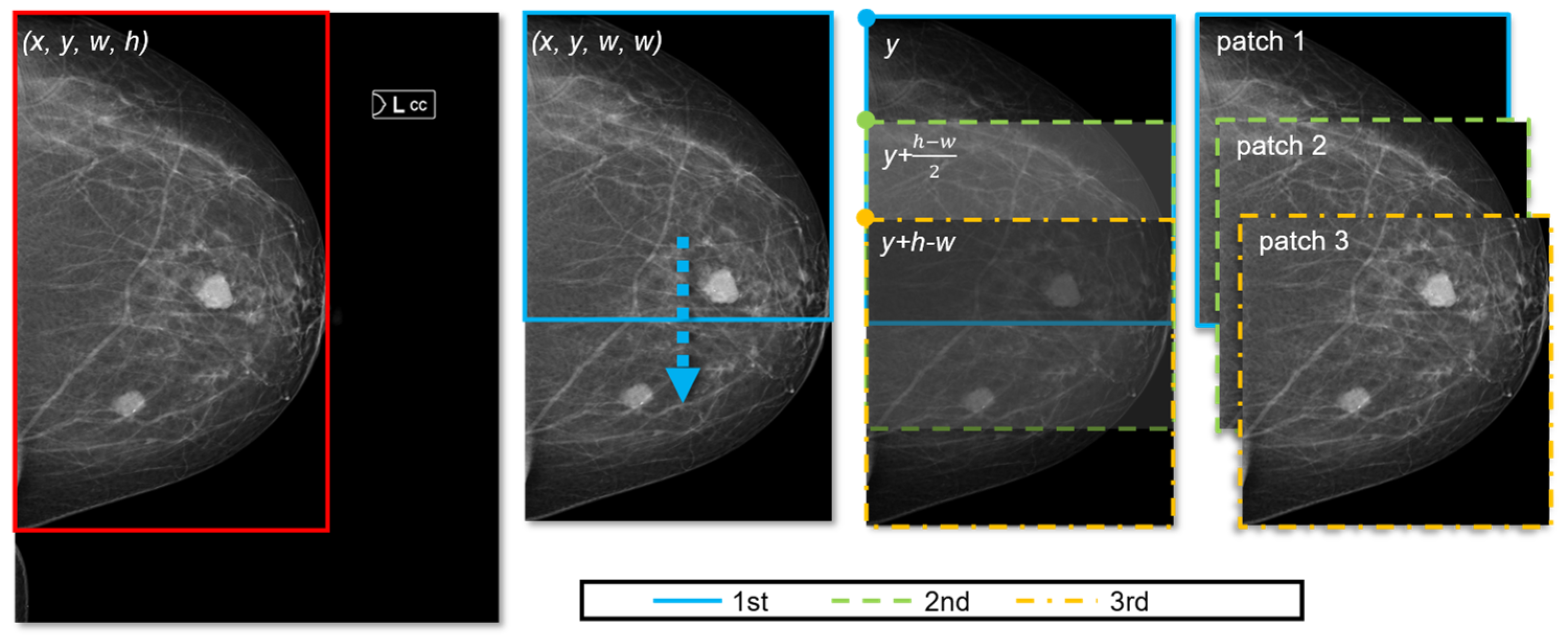
In the majority of mammogram images, 32% to 56% pixels are background pixels, which do not add any contribution to breast cancer diagnosis. Therefore, we can crop the breast region accurately using image processing tools. This image processing step inputs the original mammogram and outputs extracted bounding box (x, y, w, h), where x, y represents the top-left coordinate of the box and w and h denote width and height of the box, respectively. Given that all breast masses and micros (e.g., cysts, calcification) are included inside this extracted area, it can serve as our primary RoI.

Next, using the obtained bounding box for the breast region (x, y, w, h), we generate n square patches. Figure 2 illustrates how square patches are obtained from the extracted breast area (for simplicity, only the case of h > w is presented in the figure). When h > w, all patches are generated by sliding down the square box vertically (from top to bottom), meaning that the x coordinate does not change. Moreover, since we generate square patches, their width and height are the same (i.e., both are w). Hence, to represent each patch, only y coordinates are computed. First, the number of patches, n, is determined by Equation (1).

$$n=max\left(\left[w/h\right]+1, \left[h/w\right]+1\right)$$

(1)

where $max$ (·) is a function that returns the maximum of values and [·] denotes a standard rounding function. The increment (“+1” term) in the equation assures each tumor is included within at least one square patch. The details of patch generation are shown in Algorithm 1. The coordinates of the first and last patches are known (lines 4–5 and 10–11); therefore, depending on n, the remaining patches are computed. In a similar fashion, when h < w, we move the square horizontally (from left to right) to generate patches (i.e., both width and height are h; the y coordinate does not change; x changes according to n), as shown in lines 10–14.

Algorithm 1: Square patch generation
1:	Input: n, (x, y, w, h)
2:	Output: list of bounding boxes, bbox[]
3:	if h > wthen
4:	bbox[0] ⃪ x, y, w, w
5:	bbox[n - 1] ⃪ x, y + h - w, w, w
6:	for i = 1 to n − 2 do
7:	bbox[i] ⃪ x, y + i × (h − w)/(n − 1), w, w
8:	end
9:	else
10:	bbox[0] ⃪ x, y, h, h
11:	bbox[n - 1] ⃪ x + w - h, y, h, h
12:	for i = 1 to n − 2 do
13:	bbox[i] ⃪ x + i × (w − h)/(n − 1), y, h, h
14:	end
15:	end

3.2. Tumor Detection

After we obtained all patches, breast tumors are detected using object detection methods. Generally, any state-of-the-art object detection model can be employed, such as You Only Look Once (YOLO) [23], SSD [16], Region Based Convolutional Neural Network (R-CNN) [24,25] models, and their variants. In our study, Faster R-CNN [25] is used as it performed slightly better than YOLO and SSD models for our dataset (refer to

Table 2. Detection accuracy comparison between popular object detection models.

Method	Recall	Mean IoU
Mask R-CNN	0.932	0.59
Faster R-CNN	0.954	0.63
YOLO	0.938	0.48
SSD	0.95	0.55

). Moreover, Mask R-CNN [24] is also another option to consider as it can determine corresponding masks (segmentation) for detected tumors, which can be useful for medical reporting.

All generated patches from the previous step are fed to the Faster R-CNN model to obtain corresponding bounding boxes, class names, and confidence scores for detected masses. However, these bounding boxes represent detected tumors for the patches (i.e., corresponding to generated x, y coordinates). Therefore, we need to map these bounding boxes to locate breast tumors on the original image. Given the original image boundaries, each detected tumor (let us denote i-th detection as x’_i, y’_i, w’_i, h’_i) is mapped to the original image using Equation (2):

$$\begin{gathered} x_m{}_i :=x{’}_i+x \\ y_m{}_i :={y^{\prime }}_i+y \\ {w}_m{}_i :={w^{\prime }}_i \\ {h}_m{}_i :=h{’}_i \end{gathered}$$

(2)

where (x’_i, y’_i, w’_i, h’_i) represents the i-th detection corresponding to the extracted breast area with a bounding box of (x, y, w, h). Thus, the mapped bounding boxes are denoted by ($x_m, y_m, w_m, h_m$).

Since multiple patches are used to detect breast tumors, some tumors might be present in more than one patch. The duplication removal algorithm is used to find the unique bounding box for each tumor. Algorithm 2 describes the duplication removal process in detail. Our duplication removal algorithm is inspired by how conventional object detection models handle multiple detections for the same object. We use an intersection over union (IoU) threshold of 0.5, obtained by the original Faster R-CNN model. Lastly, we locate the unique detections on the original image to derive the final output.

Algorithm 2: Duplication removal
1:	Input: list of detections, det[]
2:	Output: updated list, newDet[]
3:	newDet  ⃪ det[0]
4:	noDuplicate ⃪ True
5:	for i = 1 to len(det) – 1 do
6:	for j = 0 to len(newDet) – 1 do
7:	Compute IoU for bbox[i] and bbox[j]
8:	if IoU ≥ 0.5 then
9:	if conf[i] > conf[j] then
10:	Replace newDet[j] with det[i]
11:	end
12:	noDuplicate ⃪ False
13:	end
14:	end
15:	if noDuplicate then
16:	Append det[i] to newDet
17:	end
18:	end

3.3. Intra-Class Classification Improvement

Having a separate classification model to boost the performance of the detection models is not a new approach in literature of medical diagnosis. Through a comprehensive survey on DL-based breast cancer diagnosis approaches, Mridha et al. [26] showed that artificial neural networks (ANN) [27], deep belief networks (DBN) [28] as well as CNN models can help CAD systems improve the classification accuracy by solely focusing on unique and deep features of detected tumors. In this study, we employ a standalone CNN-based classification model to combine its softmax scores with the detection model’s classification scores. As shown in Figure 1, this classification model receives detected tumors (which are the outputs of the detection model) as inputs and performs an inference to classify the type of the tumor. However, first, detected tumors should be upscaled as shown in Figure 3. Note that CNN classification takes place after we find unique bounding boxes for each tumor by mapping back and removing duplication from generated patches. Figure 3 shows the rescaling of bounding box coordinates, which, evidently, is crucial for the classification model.

Empirically, we found out that rescaling the bounding box by a factor of 1.7 improves the classification accuracy the best compared to other rescaling factors (e.g., 1.5×, 2×). Although there is no exact design for the rescaling factor, having healthy tissue around the tumor helps the classifier identify the type of tumor better. In our study, 65% of healthy tissue and 35% of the detected breast tumor achieved the highest accuracy (scaling factor of 1.7 is derived by this idea). This notion is also presented by Singh et al. [15], where they concluded that around 70% of healthy tissue along with the segmented tumor increases tumor shape classification accuracy.

We propose two CNN-based classification models with 256 × 256 and 128 × 128 input sizes to avoid information loss in downsampling of bigger breast tumors. Detected tumors are downsampled to one of two input sizes according to their initial size. The smaller model consists of three convolutional layers, followed by two fully connected layers. The kernel size for the first convolutional layer is 5 × 5, and, for the rest, 3 × 3. The size of the first and the second fully connected layers are 128 and 6 (the number of classes). After the flattening and the first fully connected layers, we used dropouts of 0.2 and 0.3, respectively. We used the ReLU activation function for all layers except the output layer, where softmax is used. The network with 256 × 256 input size follows the same structure as the smaller network. The difference is that this network contains one more convolutional (kernel size of 3 × 3) and max pooling layers prior to the fully-connected layers. We trained both networks with their corresponding inputs (e.g., upscaled bounding box by a factor of 1.7, as explained above) on our private dataset to achieve classification accuracy of 0.95 for both networks. In the experiment section, we show how this model improves the overall mean average precision of our proposed DL model.

3.4. Transfer Learning

In the previous subsections, we discussed the overall flow of the proposed deep learning method from RoI generation, to improving classification accuracy of the object detection model with the help of a CNN-based classifier. All procedures are firstly performed on our private dataset as it has more and higher quality mammograms. Using the pre-trained model, we aim to fine-tune the network parameters for the INbreast database. However, before starting training on this dataset, some pre-processing procedures should be done. Firstly, two datasets contain mammograms with different intensities and contrast. Figure 4 shows two samples from each database for reference. In order to reduce the dataset difference for more accurate adoption, we enhance the texture and contrast (e.g., using CLAHE [29]) of INbreast mammograms. These pre-processing steps take place after breast region extraction but before square patch generation. Figure 5 shows samples before and after pre-processing operations. As seen from Figure 5b, the enhanced image now displays clear tissue information and is quite similar to mammograms in our private dataset.

Secondly, the INbreast database contains annotated RoI (segmentation) for each mammogram. Using corresponding files, segmentation contours are also converted into bounding boxes (XLM format), just like in our own private dataset, to directly apply the network for INbreast mammograms. For comparison purposes, we follow prior literature [10,15,17] and exclude patient studies with BI-RADS 3, and assign all images with BI-RADS 4, 5, 6 as positive samples and BI-RADS 1 and 2 as negative samples. Finally, we compare the experiment results with existing works.

Both Faster R-CNN and CNN-based classifiers are fine-tuned on the INbreast dataset. The training process follows the same procedures as discussed before (i.e., breast region extraction, image enhancement, square patches generation, bounding box mapping, duplication removal).

4. Experimental Results and Discussion

Our experimental evaluation has three major objectives. The first objective is to evaluate the detection accuracy of the Faster R-CNN model in comparison to other state-of-the-art object detection models. Since the performance of tumor classification is heavily dependent on breast tumor detection, we need to assure that all tumors are present in at least one of the generated patches. To this extent, we also need to check if the entire breast region is clearly extracted from the original mammogram. The second objective is to show the overall performance improvement of the proposed model over conventional detection algorithms (e.g., original Faster R-CNN). This validates the importance of square patches generation (RoI) since we train the original Faster R-CNN model on the whole image. To this extent, we demonstrate comparisons between our method and the original Faster R-CNN model. The third objective is to transfer the model knowledge for the INbreast database and conduct comparison experiments with existing breast cancer diagnosis approaches. All experiments are conducted using 2× NVIDIA Tesla V100 32GB GPUs. Training in our machine took about 27 h. In addition, the inference time takes less than 4 s for each request (inputted mammogram), which is satisfactory because breast cancer diagnosis does not require real-time processing.

Firstly, it is important to report that breast area extraction in the first stage extracted breast area with mean IoU of 0.91 and standard deviation of 0.014 for training samples. When cross-referenced against annotated tumor data, a zero bounding box was found outside the extracted breast region, which means that the first pre-processing step was successful in accurately extracting the breast region from the whole mammogram image. Next, square patches are generated using 1567 training data, and object detection models are trained on these patches (patches not including an annotation are excluded from training). Table 2 shows the detection accuracy of state-of-the-art object detection models. For our dataset, Faster R-CNN performed the best, followed by the SSD detection model. YOLO has better recall but lower mean IoU score compared to Mask R-CNN, which can be due to anchor limitations for each selected grid. In this study, computational complexity is not a main concern. In addition, since Faster R-CNN achieved the best results, we carry on following experiments using Faster R-CNN. Furthermore, because Mask R-CNN has a built-in masking (segmentation) module, it is interesting to examine its performance further.

In the second part of the experiment, we compare the performance of detections using the BI-RADS lexicon. The object detection model is trained on 4124 patches generated from training data of 1567 mammography images. The remaining patches that do not contain any labeled masses/micros are discarded. In addition, for comparison, we trained the original Faster R-CNN model on 1567 whole mammogram images. To ensure fairness, we trained both models for 300 epochs on the same training conditions (e.g., the same GPU and machine). Figure 6 shows the results of our two-stage model and the original Faster R-CNN model on sample images. It is seen that our two-stage model can detect BI-RADS 2 far better than the ‘one-stage’ model because more information can be preserved by generating patches from extracted RoI. This validates that our method effectively solves the issue of the huge ratio difference of small lesions to the original input size by avoiding the proportion of breast lesions from being underrepresented. Moreover, our model eliminates false detections, which contributes to significant performance improvement, as seen in Figure 6a where original Faster R-CNN falsely detected BI-RADS 4.

Figure 7 shows the performance difference between our proposed two-stage method and the original Faster R-CNN model for each BI-RADS category. The difference is especially significant for BI-RADS 2 due to its very small size in comparison to the overall input image. Our method detects 439 more BI-RADS 2 and 3 classes compared to Faster R-CNN. In addition, it is clearly seen across all classes that our method outperforms the original Faster R-CNN model in terms of accuracy. For instance, our method correctly classified 23% of BI-RADS 4 classes (4a, 4b, and 4c). Lastly, the precision of BI-RADS 5 and 4c improved by 7%, which is substantial considering their importance (e.g., BI-RADS 5 yields high suspicion of malignancy with a 95% chance of breast cancer). Overall, the mean average precision (mAP) improved from 0.85 to 0.92 with IoU of 0.45 (i.e., 0.92 [email protected]). From the results, it is seen that our two-stage method that generates smaller patches and then uses them to obtain combined final detections proves to be efficient.

Table 3. Confusion matrix for BI-RADS scores. The values are normalized so each row sums to one.

		Predicted Results
		Background	2	3	4a	4b	4c	5
True Data	Background	0.90	0.05	0.02	0.02	0	0.01	0
	2	0.14	0.78	0.08	0	0	0	0
	3	0.07	0.05	0.88	0	0	0	0
	4a	0.01	0	0	0.96	0.02	0.01	0
	4b	0	0	0	0.02	0.96	0.01	0.01
	4c	0	0	0	0.01	0.03	0.96	0
	5	0.01	0	0	0	0	0.01	0.98

shows the confusion matrix for our model, where classification for each BI-RADS categories can be seen clearly. BI-RADS 2 is most likely to be misclassified as background and sometimes as BI-RADS 3. Furthermore, BI-RADS 5 achieved the best performance, which is desirable considering its importance.

Moreover, by employing a supportive classification model, the accuracy for intra-classes improved by another 0.02 mAP.

Table 4. Mean average precision of classification models.

Method	mAP
Faster R-CNN	0.92
Classification model	0.93
Combined results	0.94

shows the performance of the Faster R-CNN classifier, CNN-based classification model, and their combined results. Overall (combining two models), our method achieved 0.94 [email protected].

Similarly, experiments with Mask R-CNN showed overall performance improvement from 0.83 (original Mask R-CNN model) to 0.92 mAP (our two-stage model with Mask R-CNN). However, Faster R-CNN outperforms Mask R-CNN, and the utilization of Mask R-CNN in real-world CAD systems can be useful for medical reporting because the model can generate masks along with detection bounding box coordinates. These experiment results prove that our patch generation method in the first stage improves the accuracy of detection and classification, especially for the detection of very small breast abnormalities (Figure 7).

In the last part of the experiment, we perform transfer learning. We use our pre-trained model (trained on our private dataset) to learn features of INbreast database samples via fine-tuning. The proposed model achieved an AUC (i.e., area under the curve) score of 0.97.

Table 5. The overall performance comparison with existing methods on the INbreast dataset.

Method	Network	End-to-End	Fully CAD	Accuracy	AUC
Dhungal et al. [30]	CNN	No	No	0.95	0.91
Zhu et al. [31]	MIL	Yes	No	0.90	0.89
Shams et al. [17]	GAN + CNN	Yes	No	0.935	0.925
Singh et al. [15]	SSD + cGAN	Yes	No	0.80	-
Shen et al. [10]	CNN	Yes	No	-	0.95
Our model	R-CNN + CNN	Yes	Yes	0.95	0.97

shows comparison results with existing methods on the INbreast database. Among all compared methods, only our method can directly be used to assist radiologists, since we train our classifier to identify standard BI-RADS categories. By automatically generating small patches from the original mammogram, our method can focus on smaller RoI to improve the detection accuracy. Moreover, appropriate data processing tools contributed to accuracy improvement, especially, for the INbreast dataset (due to intensity and contrast differences). Our model achieved the highest accuracy and AUC scores of 0.95 and 0.97, respectively.

In addition, with the support of a classification network, we improved the overall accuracy of the model. Although it did not contribute a lot for the INbreast dataset (due to binary classification), in our private dataset, the model’s mAP is improved from 0.92 (without the CNN model) to 0.94 (with CNN) across six BI-RADS categories. This proves that our CNN based-model helps identify key feature differences for intra-classes (e.g., BI-RADS 4a vs. 4b).

In Table 5, corresponding results of compared methodologies are obtained by their study reports. Among methodologies that use the whole mammogram images, the DiaGRAM method proposed by Shams et al. [17] achieved the best results. However, we believe more and more research studies should focus on better ways of generating smaller RoIs and avoid using the whole mammogram, as the size of the medical imaging gets bigger and bigger with the advancement of high-resolution input modalities. Clear evidence can be seen from the resolution and the quality differences between the DDSM database, which contains digitized film mammograms and INbreast, which is fully digital. In comparison, mammograms in our collected dataset have twice the resolution of INbreast images.

5. Conclusions

In this paper, we propose a two-stage deep learning method for breast cancer detection using high-resolution mammograms. Our method does not require any human supervision or manually annotated RoIs to perform accurate detection for in-the-wild data. Experimental results on the collected mammogram dataset demonstrate significant improvement over the original Faster R-CNN model. Our model does not only improve detection accuracy for BI-RADS categories but also improves classification accuracy by combining output scores with a specifically-designed tumor classifier. In addition, due to the contribution of generated patches, the model reduces false detections. Using square patch generation, bounding box mapping, and duplication removal algorithms, our method could achieve near-optimal detection accuracy on the labeled test data. Moreover, through extended comparisons with the existing breast cancer diagnosis methods on the publicly available INbreast dataset, we showed the superiority of our model. Our proposed model can be used to assist radiologists in real-world breast cancer screening and reporting.

Even though our CNN-based classifier improved the overall performance, there are still a few misclassified intra-class scores (BI-RADS 4a and 4b). In the future work, we aim to design better standalone classifiers by thoroughly experimenting on different network architectures.