A Comparative Study of Two Rule-Based Explanation Methods for Diabetic Retinopathy Risk Assessment

Abstract

Understanding the reasons behind the decisions of complex intelligent systems is crucial in many domains, especially in healthcare. Local explanation models analyse a decision on a single instance, by using the responses of the system to the points in its neighbourhood to build a surrogate model. This work makes a comparative analysis of the local explanations provided by two rule-based explanation methods on RETIPROGRAM, a system based on a fuzzy random forest that analyses the health record of a diabetic person to assess his/her degree of risk of developing diabetic retinopathy. The analysed explanation methods are C-LORE-F (a variant of LORE that builds a decision tree) and DRSA (a method based on rough sets that builds a set of rules). The explored methods gave good results in several metrics, although there is room for improvement in the generation of counterfactual examples.

1. Introduction

Healthcare costs are continuously raising, due to the increase of life expectancy, the improvements in the management of chronic diseases and the development of new treatments. Diabetes Mellitus (DM), suffered by 382 million adults worldwide, is one of the most important chronic diseases. DM patients are estimated to increase up to 592 million adults by 2035 [1]. Moreover, specialists estimate that around 46% of diabetic patients have not been diagnosed [1]. DM has been growing steadily in the last few years. In Spain, the National Health Survey (NHS) detected that diabetes increased from 4.1% of the population in 1993 to 6.4% in 2009. Specialists predict an incidence of more than 3 million DM patients in Spain by 2030 [2].

Diabetic Retinopathy (DR) is an ocular disease related to DM. It is the main cause of blindness and visual impairment worldwide and the most common among working-aged adults [3]. Overall, DR affects 30% of diabetic patients, 11% show some degree of vision loss (sight-threatening diabetic retinopathy [4]), and 4% lose their sight completely. However, early detection through periodic screening can reduce this risk by as much as 95%.

Artificial Intelligence (AI) techniques may improve the screening quality by identifying the patient’s risk of developing DR using information from the Electronic Health Record. In the healthcare domain, it is common to build clinical decision support systems (CDSS) using Machine Learning (ML) tools and algorithms. These intelligent CDSS assist clinicians in diagnosing diseases and choosing treatment decisions.

Recently, we observed significant and continuous success in the development of ML-based systems. Such success is attributed to many factors, including the presence of vast amounts of data, the advances in ML and the affordability of more advanced computer equipment. As a result, ML-based systems have become ubiquitous in our society and regular life, and a vital component of multiple applications in many domains, including healthcare.

In line with this progress, our research group and the Ophthalmology Unit of the University Hospital Sant Joan (Reus, Tarragona) have developed a CDSS called RETIPROGRAM [5,6], that helps clinicians to estimate the personalised risk of developing DR as early as possible. The AI core of RETIPROGRAM is a Fuzzy Random Forest (FRF) composed of 100 Fuzzy Decision Trees (FDTs). A FDT is a hierarchical structure that classifies patients based on the values of a set of attributes related to DR risk factors. Each node of the tree represents an attribute. A branch of a node is associated to a possible value of that attribute. Finally, the tree leaves assign patients to two categories: patients with/without risk of developing DR. Each branch is a rule, that provides a result if the attributes have certain values. Experimental results have shown that the system could be incorporated in DR screening programs and improve the quality of screening models [7].

However, it is known that, in domains such as healthcare, high precision is not enough to convince society to trust the decisions of ML-based systems. When a decision is made or suggested by an automated system, it is crucial for practical, social, and increasingly legal reasons to explain the rationale behind that decision to users, developers or regulators. In the case of RETIPROGRAM, a patient may want to know why she has a high risk of developing DR, so that she can try to change her lifestyle to reduce it.

As a result, we started to develop methods to derive explanations for the predictions of the RETIPROGRAM system. In the literature, we can find a variety of techniques to achieve this goal. The simplest solution is to directly inspect the components of the models—e.g., the activated path in a fuzzy decision tree. However, such a naive solution is not feasible in the case of random forests with hundreds of trees. The internal structure of such models is complex, and it is not easy to be inspected. Alternatively, we can develop post-hoc explanation methods [8]. Such methods aim to study the relationship between the input and output produced by the system to explain and extract post-hoc explanations. Most of the explanation methods that follow this approach generate a set of inputs, analyse the answers provided by the system to be explained and then create a simpler model from which we can infer an explanation [9,10,11].

The most well-known examples of post-hoc ML explanations are Local Interpretable Model-agnostic Explanations (LIME) and Local Rule-Based Explanations (LORE). LIME provides local explanations for a classifier’s prediction by fitting a linear regression model locally around the data point of which the prediction is to be explained. LORE generates a set of neighbours of the input point, applies the classification system to them, and builds a decision tree on these results. The explanation obtained by the LORE method is composed of two parts: the activated path, i.e., the rule used to produce the decision, and a set of counterfactual rules which represent the minimal number of changes in the feature values of the instance that would change the conclusion of the system. So, the main difference between LIME and LORE is the neighbourhood generation procedure and the type of explanations each derives.

In a previous work [12] we proposed Guided-LORE, an adaptation of the LORE method in which the neighbourhood generation, which is the key in obtaining a solid explanation, was formalised as a search problem and solved using Uniform Cost Search. Such adaptation allowed us, to some extent, to make the generation process more informed. However, we found that both LORE and Guided-LORE did not take into consideration explicitly the case in which the attributes that define the objects are fuzzy. For example, when we use Guided-LORE, a neighbour of a point is generated by adding (or subtracting) a fixed amount (which is called step) to the value of an attribute. We addressed these shortcomings by proposing C-LORE-F (Contextualized LORE for Fuzzy attributes) [13]. If we know that an attribute is fuzzy and we have the information on its fuzzy labels and their associated fuzzy sets, we can make a more focused neighbourhood generation. Based on the definition of the fuzzy sets of each attribute, we can generalise its step from being a fixed value to being a function that depends on that knowledge. In that way, the proposed method is more general. It works in cases where the fuzzy sets associated with the linguistic labels are uniformly or non-uniformly distributed. To the best of our knowledge, that work was the first one that considered such knowledge to develop explanation methods for ML systems based on fuzzy logic, e.g., Fuzzy Decision Trees and Fuzzy Random Forests [14].

In this work, we study two different ways of generating rules in the C-LORE-F method. On one hand, we use the classic crisp decision trees. On the other hand, we propose the construction of preferential decision rules based on rough sets (using the Dominance-Based Rough Set Approach, DRSA, [15]). Both methods are used to generate explanations for the RETIPROGRAM classifier.

The rest of this article is structured as follows. Section 2 provides an overview of the related works. In Section 3, we present the two rule explanation methods used in this comparative work. Section 4 presents a general framework for generating counterfactual-based explanations for the RETIPROGRAM classifier. The focus is on the methods for obtaining the decision rules that are used to generate the explanation. In Section 5 we describe the experimentation, including several tests to evaluate and compare the performance of both methods. Finally, in Section 6, we conclude the paper and list some points for future work.

2. Literature Review

Although it is possible to consider machine learning-based systems as reliable, their effectiveness is restricted by the lack of explanation of their decisions and actions to end-users. So, in the literature, we find an increasing body of work on interpretable and transparent Machine Learning algorithms in general, especially applied to sensitive domains such as healthcare. This section provides a brief literature review about the work on explanation methods.

Recently, the research of methods for explaining the output of black-box decision systems has got critical attention [16], and there has been an extraordinary amount of articles in ML interpretability in the last years. We can categorise the works on ML interpretability into those based on features’ importance (Section 2.1), counterfactual examples (Section 2.2) and visualisation mechanisms (Section 2.3).

2.1. Methods Based on Measuring the Importance of Features

There are two main directions for developing explanation methods based on the importance of features, global and local explanation methods. Global methods try to explain the entire model behaviour using surrogate models, whereas local models explain a single prediction. It can be helpful, in some scenarios, to understand the global logic of a model. However, the major issue with such approaches is that, as the explanations are extracted from simpler surrogate models, there is no guarantee that they are faithful to the original model [8,11,17].

Local explanation methods are arguably the fundamental approaches to the construction of post-hoc explanations. LIME [11], already mentioned in the introduction, is a well-known example. It is independent of the type of data and the black box to be explained. Given a black box model b, an instance x, and a decision y produced by b on x, LIME constructs a simple linear model that approximates b’s input-output behaviour to justify why b predicts y. It generates some neighbours of x randomly in the feature space centred on x. Such an approach is becoming a conventional method. We can find now LIME implementations in multiple popular packages, including Python, R and SAS.

The authors of LIME observed that it does not measure its fidelity. As a result, the local behaviour of a notably non-linear model may lead to faulty linear approximations. Hence, they were motivated to work on a new model-agnostic method, Anchors, based on if-then rules [18]. This method highlights the part of the input that is adequate for the classifier to make the prediction, delivering more intuitive and easy-to-understand explanations.

SHAP [19] is a method that provides an explanation of the prediction of the output of a black box for an instance x by estimating each feature’s contribution to that prediction. These contributions are collected by measuring the Shapley values from coalitional game theory. The features act like players in a coalition. Each player can be formed by a single feature or a subset of features. The Shapley values show the payout distribution of the prediction among the features.

2.2. Methods Based on Counterfactual Examples

Another important category of explanations is based on the generation of counterfactuals. The methods of this approach seek minimal changes to the feature values such that the model’s predicted outcome changes. Such kind of explanations can be helpful in different scenarios (e.g., an applicant for a bank loan might want to know which part of her application could be changed to get her application approved).

The work presented in [20] is considered to be the first one that employed the counterfactual examples to provide an explanation for the decisions of a classifier. It used a heuristic best-first search to develop a model-agnostic method for finding evidence counterfactuals that can explain the predictions of any classification model. LORE [21] is another example of this approach that is more related to our work, although it can also be seen as an example of the determination of features’ importance. It constructs a decision tree c based on a synthetic neighbourhood of the input point generated by a genetic algorithm. Then, an explanation e, composed of a decision rule and a set of counterfactual rules, based on some extracted counterfactual examples, is obtained from the logic of c. The authors in [22] developed a general optimisation framework to generate sets of diverse counterfactual examples for any differentiable Machine Learning classifier. Russell proposed in 2019 what is called a “mixed polytope”, a set of constraints that can be used with integer programming solvers to extract counterfactual explanations without making a brute-force enumeration [23].

2.3. Methods Focused on Visualisation

Visualisation-based interpretation methods play an essential role to show comprehensible explanations. We can find several visualisation methods proposed in the literature to help ML engineers and domain experts to understand, debug, and refine ML models. For example, the work presented in [24] proposed an interactive visualisation method to help users, even those without expertise in Machine Learning, to understand, explore and confirm predictive models. This method by Ming et al. extracts a set of rules that approximates a classifier’s prediction and visualises them using an interactive visual interface. Neto and Paulovich proposed Explainable Matrix (ExMatrix) [25], a visualisation method to interpret Random Forests. They used a matrix as a visual metaphor in which rows represent rules, columns are features, and cells are rules predicates. They showed that their method is capable of offering global and local explanations of Random Forest models.

3. Preliminaries

This section provides a brief background about Contextualised LORE for Fuzzy attributes (C-LORE-F), which uses classic decision rules, and the Dominance-based Rough Set Approach (DRSA), that builds a set of rules taking into account the preference direction of the variables.

3.1. Contextualised LORE for Fuzzy Attributes (C-LORE-F)

C-LORE-F is a variant of the LORE and Guided-LORE methods for fuzzy-based ML models. It provides an explanation for the decision assigned to a specific instance based on some contextual information (e.g., the type of attribute and the fuzzy sets associated to the linguistic values of the fuzzy attributes). The inputs of C-LORE-F are a trained fuzzy-based ML model, b, and an example x. Algorithm 1 shows the main steps of C-LORE-F. First, we apply b to x to get a decision y. We obtain a set of neighbours of x, D, and a rule-based model t is built by considering the output of b in these points. From this model t it is possible to derive an explanation, that contains the rule r used to classify x, a set of counterfactual rules $\delta$ and a set of counterfactual instances $\mathbb{C}$.

Algorithm 1:C-LORE-F

input :x: an instance to explain, T: an auxiliary set, b: a black-box model, L: maximum level of exploration, and $KB$: knowledge base.    output: E: the explanation of the decision of b on x 1 $y\leftarrow b\left(x\right)$; 2 ${\mathcal{D}}^{+}\leftarrow GetNeighbours(x,y,b,L,KB)$; 3 $x^{-},y^{-}\leftarrow FindDiffExample(x,y,b,T)$; 4 ${\mathcal{D}}^{-}\leftarrow GetNeighbours(x^{-},y^{-},b,L,KB)$; 5 $\mathcal{D}\leftarrow {\mathcal{D}}^{+}\cup {\mathcal{D}}^{-}$; 6 $t\leftarrow BuildModel(\mathcal{D},b)$; 7 $r=(p\to y)\leftarrow ExtractRule(x,t)$; 8 $\delta \leftarrow ExtractCounterfactualRules(x,r,t)$; 9 $\mathbb{C}\leftarrow ExtractCounterfactuals(x,\delta ,t)$; 10 $E\leftarrow (r,\delta ,\mathbb{C})$

The set $\mathcal{D}$ is obtained by merging two subsets, ${\mathcal{D}}^{+}$ and ${\mathcal{D}}^{-}$. The first one is called the positive set, and it contains a set of instances that belong to the same class of x. The second one, the negative set, contains examples with a different class. We obtain ${\mathcal{D}}^{-}$ by looking at an auxiliary set T and finding the closest example to x, i.e., $x^{-}$, that has a different label than y. T can be the training set used to train the black-box model, if accessible, or any other data set from the same distribution.

The neighbours generation step is the key point in C-LORE-F and similar methods. As a first change with respect to LORE and Guided-LORE, we have defined the following types of attributes.

• Attributes with a fixed value (e.g., sex).
• Attributes whose value increases in time (e.g., age).
• Attributes whose value decreases in time (e.g., years left until retirement).
• Variable attributes, that can change positively and negatively (e.g., weight).

The motivation of such definitions is to generate useful and actionable explanations. For example, nobody can reduce his/her age, so it is not useful to give a counterfactual rule saying “if you were 10 years younger, your risk of developing DR would be much lower”.

We define the neighbourhood generation as a search problem in which we explore the neighbourhood space of a point x by applying a Uniform Cost Search based on the Heterogeneous Value Difference Metric (HVDM, [26]), using some contextual information about the attributes (e.g., the attribute type and the fuzzy set definitions). This search problem can be formulated as follows:

• State Space: the set of all possible examples S.
• Initial State: $(x,y)$, where x is the instance of which we want to generate its neighbours and y is the label of this instance obtained by the black-box b.
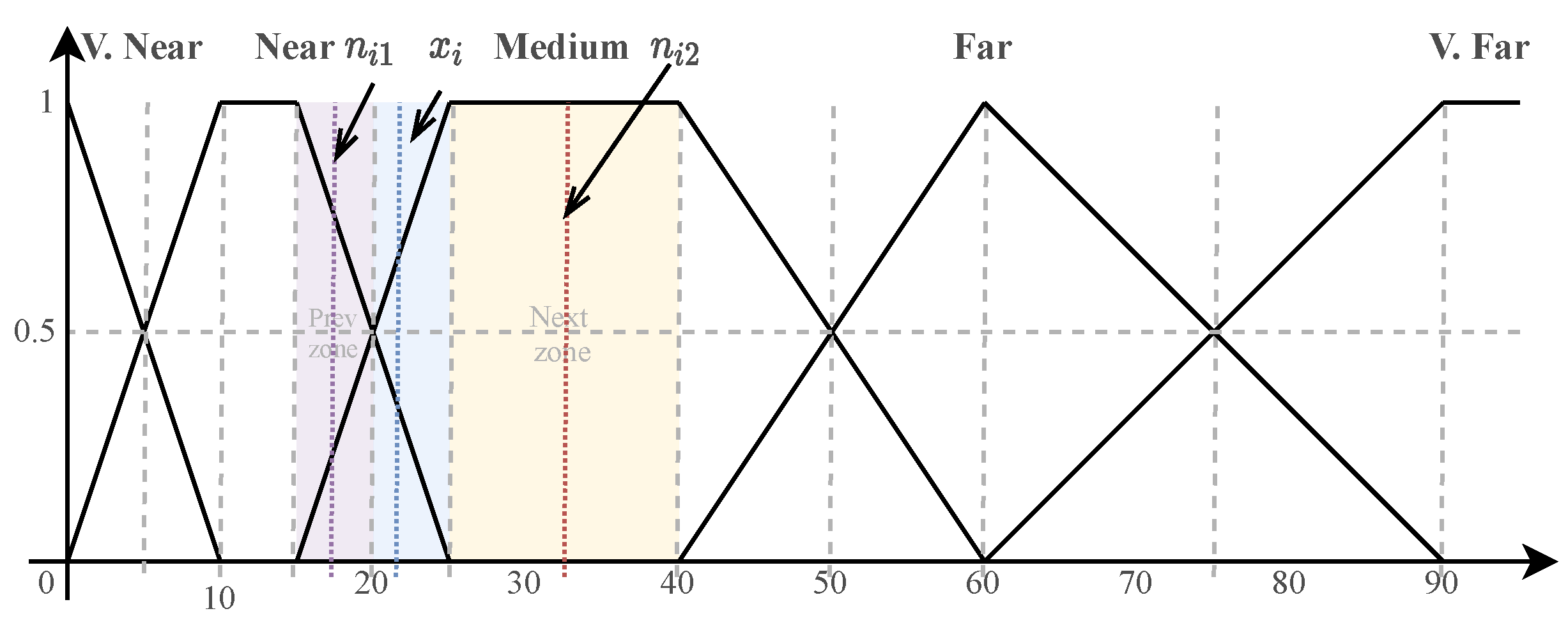
• Actions: Modifications of the value of a single attribute (feature). These actions leverage some contextual information about the feature to make the desired changes to generate new neighbours. In our case, we define two types of actions, next and prev, described later.
• Transition Model: returns a new instance in which the value of a feature is changed by applying all actions.
• Goal Test: We check, for each generated individual, if, according to the black box, it has the same label as the root, y. If that is the case, we generate its neighbours in the same way (i.e., applying one positive/negative change in the value of a single attribute). Otherwise, we have found an individual close to x that belongs to another class; thus, we have reached a boundary of y, and we terminate the search from that instance.
• Path Cost: The path cost of each example is calculated by measuring the HVDM distance between the generated example and x.

Hence, the generation of the closest neighbours of an instance x is a tree search procedure. The search process starts from this instance, and the available actions to move from one instance to another are applied. For each feature f, the number of possible actions can be zero (f is Fixed), one (either next if the feature is temporally increasing or prev if it is temporally decreasing) or both, if f is variable. Each action only changes the value of one feature.

The candidate node to be expanded, n, is the one closest to x, based on the path cost. If the outcome of the black-box model for the instance in n is different from y, then it is a leaf of the tree. Otherwise, we expand that node. Consequently, for each node in the second level, we would have changes in two attributes or double changes in the same attribute, and so on. The expanding process terminates when we reach a predefined max-level, or when there are no more nodes to be expanded (all the leaves have led to changes in the initial classification). Repeated instances are ignored to avoid cycles.

The expanding process is done by cloning the instance of the node to be expanded and applying the next and/or prev actions. After that, we pass the obtained instance to the black-box model b to obtain its corresponding label.

To apply the actions step and prev for a given attribute we consider some separate zones based on its fuzzy sets, which are defined as shown in Figure 1, taking into account the intersection point between two consecutive fuzzy sets and the intervals of maximum activation.

In Figure 1 the zones would be 0–5, 5–10, 10–15, 15–20, 20–25, 25–40, 40–50, 50–60, 60–75, 75–90 and 90–100. Given the value of the attribute, we locate its zone, and then we take the middle of the previous zone as the lower neighbour (the result of the prev action), and the middle of the next zone as the upper neighbour (the result of the next action). Figure 1 shows an example. The input value is 22, which belongs to the zone 20–25. Thus, the middle of the previous zone is the lower neighbour, (15 + 20)/2 = 17.5, and the middle of the next zone is the upper neighbour, (25 + 40)/2 = 32.5. We might end up applying only either the next action, if the located zone was the first one, or the prev action, if it was the last one.

As soon as we obtain the neighbours $\mathcal{D}$, we use the YaDT system [27], an implementation of the C4.5 classification algorithm with multi-way splits of categorical attributes, to build the decision tree. Finally, from the tree we can extract a set of decision rules, one for each branch in the tree.

The rules obtained are conjunctive and use inequality conditions that check if a certain numerical input value $v_j$ for attribute $f_j$ is above or below a threshold. In case of categorical attributes, the condition is an equality. So, rules have the following format:

$$IF{f}_{i}op{t}_i[\mathrm{AND}{f}_{j}op{t}_j\dots \left[\mathrm{AND}{f}_{z}op{t}_z\right]]\mathrm{THEN}y=y_k$$

Here, $f_i$, $f_j$ and $f_z$ are attributes, $op$ is the logical condition and can be either ≤ or > if the attribute is continuous, and = if it is categorical, and $t_i$, $t_j$ and $t_z$ are thresholds.

3.2. Dominance-Based Rough Set Approach (DRSA)

The DRSA method [15] can be used to construct a set of decision rules in line 6 of Algorithm 1. The main difference of these rules with respect to those obtained from a decision tree is that they are classification rules with a set of conditions that take into account the preference directions of the input variables. In this subsection, we explain how the rules are constructed from the set of examples $\mathcal{D}$.

Rough set theory (RST) [28] is a formal theory derived from fundamental research on the logical properties of information systems. The main goal of the rough set analysis is the approximation of concepts. In addition, it offers mathematical tools to discover patterns hidden in data. As a result, it has a wide range of applications, including feature and pattern extraction, data reduction and decision rules generation (our goal in this work). It can also identify partial or total dependencies in data, among other things.

Rough set analysis concerns data stored in a table known as an Information Table. Each row represents an object $x_i$, evaluated with respect to multiple attributes representing different points of view; the information table is defined as a pair $(X,\mathcal{F})$, where X is a non-empty finite set of objects and $\mathcal{F}$ is a non-empty finite set of attributes. A special kind of information table is a Decision Table $(X,\mathcal{F}\cup Dec)$, where the attributes are divided into condition attributes $\mathcal{F}$ and decision attributes $Dec$. The former are related to features of objects, while the latter relate to decisions about objects. Often there is just a single decision attribute $\mathcal{Y}$. Distinct values $y_k$ of this attribute, called class labels, induce a partition of the set of objects into so-called decision classes $C{l}_k$.

DRSA is an extension of RST, suitable for analysis of decision tables where both condition attributes from $\mathcal{F}$ and the output decision variable (decision attribute) $\mathcal{Y}$ are ordinal, and there exist monotonic relationships between attributes from $\mathcal{F}$ and $\mathcal{Y}$. A positive relationship means that the greater the value of the condition attribute, the higher the class label. A negative relationship means that the greater the value of the condition attribute, the lower the class label. Both types of relationships are captured by induced decision rules. In general, in DRSA the number of decision classes can be more than two. Then, one has to consider upward and downward unions of decision classes. However, in the case of RETIPROGRAM, we only have two classes: 0 for the absence of DR risk and 1 for the presence of DR risk. Thus, using DRSA, we calculate rough approximations and induce decision rules for exactly these two classes.

Rules are constructed using elementary building blocks, known as dominance cones, with origins in each object in the attribute space. Based on the rough set concept, rules for a lower or/and an upper approximation of each decision class are obtained from a training set ($\mathcal{D}$ in our case) [29]. The choice of DRSA for explainability in the Diabetic Retinopathy disease is motivated by the fact that the values of the attributes are mainly ordinal, and a change from one value to another may be an indicator of the risk of developing DR. Moreover, using the VC-DomLEM algorithm [30], one can induce a set of rules being a minimal cover of consistent objects from both classes. This enables to efficiently distinguish between the two possible decision outputs [30], which is one of the aims of a surrogate model. Two types of rules may be distinguished:

• $\mathcal{Y}$ ≥ decision rules, providing lower profile descriptions for objects belonging at least to class $C{l}_k$ (so they belong to $C{l}_k$ or a better class, $C{l}_{k+1},C{l}_{k+2},\dots$):
  IF $f_1$ ≥ $v_1$ AND $f_2$ ≥ $v_2$ AND … $f_n$ ≥ $v_n$ THEN y ≥ $y_k$
• $\mathcal{Y}$ ≤ decision rules, providing upper profile descriptions for objects belonging at most to class $C{l}_k$ (so they belong to $C{l}_k$ or a lower class, $C{l}_{k-1},C{l}_{k-2},\dots$):
  IF $f_1$ ≤ $v_1$ AND $f_2$ ≤ $v_2$ AND … $f_n$ ≤ $v_n$ THEN y ≤ $y_k$.

In this notation, we must take into account that all condition attributes in $\mathcal{F}$ are considered to be maximisation functions (the higher the value, the higher the class label), which are called Gain attributes. In case an attribute has to be minimised, it is called a Cost attribute, and the lower its value, the higher the class label. It is also possible to introduce a criterion as both Cost and Gain. In this case, the attribute may appear twice in the rule and define an interval of values.

An important feature of the DRSA method coupled with the VC-DomLEM algorithm is the fact that particular rules are minimal (without redundant conditions) and the whole set of rules is non-redundant (if any rule would be removed, some consistent objects would not be covered by any rule).

Algorithm 2 shows the main steps of the DRSA method, assuming that only certain decision rules are considered (as in our case).

Algorithm 2:DRSA method

In lines 1–2, all upward and downward unions of decision classes are identified, depending on the class labels of $\mathcal{Y}$. In the loop defined in the following lines 3–5, for each upward/downward union its lower approximation is calculated. These approximations are stored inside objects representing particular unions of classes. In line 6, the quality of classification is calculated. This is a typical rough set descriptor related to consistency of data, defined as a ratio of the number of consistent objects and all objects in $\mathcal{D}$. During calculation of $\gamma$, one takes into account the lower approximations calculated previously. In line 7, the VC-DomLEM algorithm is invoked for the upward unions of classes to induce decision rules. It generates rules describing objects from the lower approximations of subsequent unions, iterating from the most specific to the least specific union to control rule minimality. Suppose decision attribute $\mathcal{Y}$ has labels $1,2,3,4,5$, and the higher the label, the more preferred the respective decision class. Then, VC-DomLEM will first generate rules for class $C{l}_5$, then for upward union of classes $C{l}_4^{\ge }=C{l}_4\cup C{l}_5$, then for upward union $C{l}_3^{\ge }$, and finally for upward union $C{l}_2^{\ge }$. Obviously, considering union $C{l}_1^{\ge }$ does not make sense (set of all objects). In line 8, the VC-DomLEM algorithm is invoked to induce decision rules for the downward unions of classes. This is realized analogously, with the only difference that this time first class $C{l}_1$ will be taken into account, then downward union of classes $C{l}_2^{\le }=C{l}_1\cup C{l}_2$, next downward union $C{l}_3^{\le }$, and finally downward union $C{l}_4^{\le }$. Remark that VC-DomLEM algorithm was introduced for the Variable Consistency DRSA (VC-DRSA), being an extension of the classical DRSA. In [30], there are four input parameters: set of upward or downward unions of classes, rule consistency measure, set of consistency thresholds for particular unions, and object covering option s (strategy). When invoking the algorithm, we set measure $\widehat{ϵ}$ [31] for rule consistency measure, supply a set of consistency thresholds all equal to zero (which forces the classical DRSA), and choose 1 for object covering option (indicating that a rule induced for any upward/downward union of classes is allowed to cover only objects from the lower approximation of that union). Moreover, in our problem (binary classification) there is just one upward union $C{l}_1^{\ge }=C{l}_1$ and one downward union $C{l}_0^{\le }=C{l}_0$. Finally, in line 9 the resulting set of decision rules is built by adding sets of rules induced for upward and downward unions of classes.

In the experiments described in this paper, we used the implementations of the DRSA method and the VC-DomLEM algorithm available in the open source ruleLearn library (https://github.com/ruleLearn/rulelearn, last access: 21 March 2022).

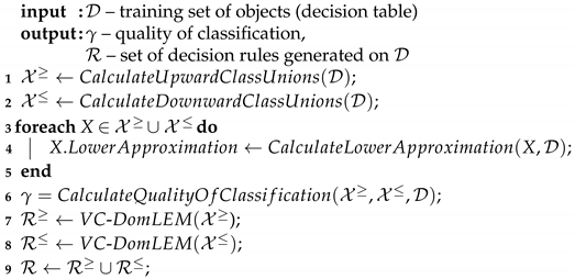
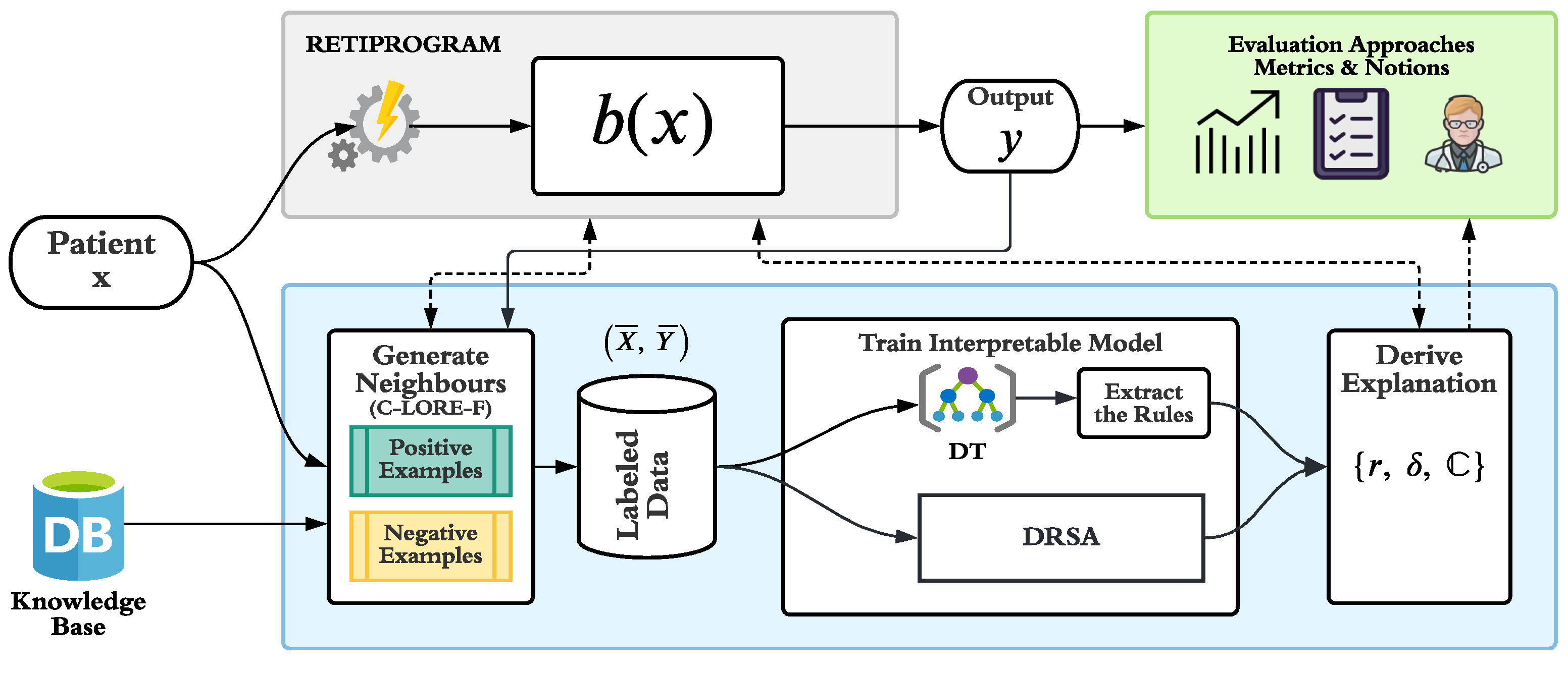
4. Explanation Generation System

In this section, we define the explanation generation methodology. Figure 2 shows the proposed architecture. Given an input x, i.e., a patient record, we first pass it to the RETIPROGRAM to obtain a class, y. Then, we pass the input x and its corresponding output y to the explanation unit (shown in the bottom part of Figure 2) to extract an explanation for that decision. The explanation unit (in blue) is composed of three parts: the neighbours’ generation module, the training module and the explanation extraction module. Finally, we forward the obtained results to the evaluation part (explained in Section 5) of the system to obtain insights into its performance.

In this article, we focus on describing the explanation and evaluation parts. We explain in detail each of these parts and their sub-modules below. For more information about the RETIPROGRAM and its development and evaluation, we refer the reader to our previous papers [14,32,33].

As we presented in Section 3, the neighbours’ generation module applies a Uniform Cost Search based on the HVDM [26] distance metric, using some contextual information about the features to generate positive neighbours (instances with the same label as x) and negative neighbours (instances with different labels than x). All of these examples are labelled using the RETIPROGRAM system, combined into one set $\mathcal{D}$ and fed to the interpretable model training module to build a surrogate model to mimic the behaviour of the RETIPROGRAM locally on $\mathcal{D}$. This model can be any simple model such as Linear Regression. However, as stated earlier, we consider two types of models in this work: a Decision Tree and Ordinal Decision Rules.

To construct the desired explanation, we first extract all decision rules from the interpretable model in the following form: IF $conditio{n}_1$ AND $conditio{n}_2$ …AND $conditio{n}_n$ THEN $decisio{n}_k$. In the case of the Ordinal Rules, we use DRSA and we obtain a minimal set of rules as output of the model training. In the case of the Decision Tree, we can derive such decision rules just following the conditions of each branch of the tree. In the case of decision trees, the selection criteria of the nodes during their construction ensures that the set of rules is small and that they use an small number of conditions. So in both cases, the generated models are much simpler than the original Fuzzy Random Forest (which has 100 trees, each one with several rules).

In the last step, we extract the explanation from these small sets of decision rules in the form of a triplet $(r,\delta ,\mathbb{C})$, where:

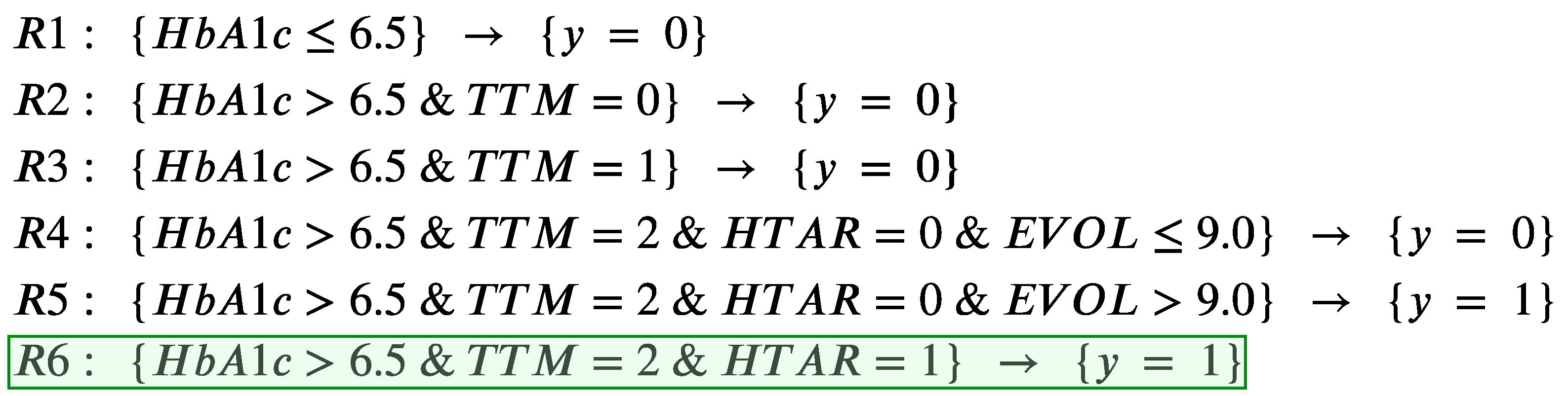
• r is the decision rule(s) that covers the instance x. This rule tells which are the necessary conditions to be satisfied by the object for being classified as y, so they indicate the minimal reasons for belonging to that class. When using DRSA, we can have more than one applicable rule with different combinations of conditions.
• $\delta$ is the set of counterfactual rules that lead to an outcome different than the one of x. They indicate the minimal number of conditions that should be simultaneously changed in the object for not being in class y.
• $\mathbb{C}$ is a set of counterfactual instances that represent examples of objects that belong to a different class and have the minimum changes with respect to the original input object x.

The counterfactual rules extraction procedure is described in Algorithm 3. It looks for all rules leading to a decision different than y and it chooses the ones with the minimum number of conditions not satisfied by x (returned by the function $nf$).

Algorithm 3:Extraction of counterfactual rules

The counterfactual examples are useful for the decision maker to understand what changes in the values of the attributes produce a change in the classification label. In Medicine, this knowledge is particularly interesting, as it can tell a patient how she could move to a better category. These instances are obtained from the counterfactual rules $\delta$ and the original input x. Given a counterfactual rule $r:q\to y$, and x, we find the instance that needs the minimum changes in x to satisfy the conditions q. We look at all the attributes in the conditions q that are not satisfied by x, and then we make the smallest change (up or down) to the values of these attributes to satisfy the conditions in q.

Let us take as an example the explanation for the patient x shown in the first row of

Table 1. Patient example and counterfactual instances.

Age	Sex	EVOL	TTM	HbA1c	CDKEPI	MA	BMI	HTAR
71.0	1	14.0	2	7.4	90.07	0.0	31.05	1
—	—	—	—	6.5	—	—	—	—
—	—	—	0	—	—	—	—	—
—	—	—	1	—	—	—	—	—

. Using RETIPROGRAM this patient is assigned to class 1. Then, the explanation system will construct the rules in Figure 3.

The activated rule r is $R6$ (the applicable one on the given patient). There are four rules that lead to the opposite decision, $Q=\{R1,R2,R3,R4\}$. Being $nf(R1,x)=1$, $nf(R2,x)=1$, $nf(R3,x)=1$, $nf(R4,x)=2$, the set of counterfactual rules $\delta$ are $\{R1,R2,R3\}$. The final step in the explanation extraction process is to construct the set of counterfactual examples $\mathbb{C}$. First we take the rule $R1$ and as its condition $(HbA1c\le 6.5)$ is false for patient x, we change its values to the smallest below the upper bound of HbA1c, which is 6.5. We repeat this process for the rest of rules in $\delta$, obtaining two other examples that only make one change in the TTM variable (as the rest of conditions are already satisfied by x). The obtained counterfactual instances are shown in Table 1 (rows 2–4), in which the empty cells mean that the initial value of that attribute is not changed. We can see that the number of changes in the counterexamples is small. In this example, changing the treatment type would decrease the risk of DR (to class 0); the other option is a decrease of the HbA1c variable, which is the glycated hemoglobin, an indicator of a bad control of the diabetes which affects the blood.

5. Experiments and Results

5.1. Experimental Setup

We evaluated the proposed explanation system on a private data set to assess the risk of developing diabetic retinopathy for diabetic patients. It is composed of 2323 examples of binary classification. The Diabetic-Retinopathy data set was used to develop a fuzzy random forest-based system, called RETIPROGRAM, which is currently being used in the Hospital de Sant Joan in Reus (Tarragona). Each instance in the data set is defined by nine attributes: current age, sex, years since diabetes detection, type of diabetes treatment, good or bad control of arterial hypertension, HbA1c level, glomerular filtrate rate estimated by the CKD-EPI value, microalbuminuria, and body mass index. The data was split into a training set of 1212 examples and a test set of 1111 examples. The classification model used in RETIPROGRAM achieves an accuracy of 80%, with a sensitivity of 81.3% and specificity of 79.7% [32]. We used the test set in all our experiments to evaluate the effectiveness of the proposed explanation system.

5.2. Evaluation of the Explanation Results

As we mentioned above, the explanation contains two main parts: first, the explanation decision rule(s), r, and second, a set of counterfactual rules, $\delta$ from which we can derive the counterfactual examples, $\mathbb{C}$. These components are obtained from a set of rules, that we call the explanation model. In this section we want to compare the quality of the rules generated by the two methods. We will denote as C-LORE-F the method using typical decision trees, and we will name as DRSA the version of the same method using rules generated with Dominance-based Rough Sets. The following evaluation metrics are used to measure the quality in both cases, for the RETIPROGRAM black-box method.

• Hit: this metric computes the similarity between the output of the explanation model and the black-box, b, for all the testing instances. It returns 1 if they are equal and 0 otherwise.
• Fidelity: this metric measures to which extent the explanation model can accurately reproduce the black-box predictor for the particular case of instance x. It answers the question of how good is the explanation model at mimicking the behaviour of the black-box by comparing its predictions and the ones of the black-box on the instances that are neighbours of x, which are in $\mathcal{D}$.
• l-Fidelity: it is similar to the fidelity; however, it is computed on the subset of instances from $\mathcal{D}$ covered by the explanation rule(s), r. It is used to measure to what extent this rule is good at mimicking the black-box model on similar data of the same class.
• c-Hit: this metric compares the predictions of the explanation model and the black-box model on all the counterfactual instances of x that are extracted from the counterfactual rules in $\mathbb{C}$.
• cl-Fidelity: it is also similar to the fidelity; however, it is computed on the set of instances from $\mathcal{D}$ covered by the counterfactual rules in $\delta$.

Table 2. Evaluation results of the C-LORE-F and DRSA explanation methods.

	Hit	Fidelity	l-Fidelity	cHit	cl-Fidelity
C-LORE-F	1.00 ± 0.00	0.99 ± 0.002	0.99 ± 0.002	0.89 ± 0.290	0.88 ± 0.282
DRSA	0.97 ± 0.152	0.831 ± 0.32	0.93 ± 0.176	0.830 ± 0.315	0.83 ± 0.298

shows the means and standard deviations of the metrics for the C-LORE-F and DRSA explanation methods on the test set. It may be seen that C-LORE-F outperforms DRSA in all metrics. Let us look at the Fidelity and l-Fidelity for the DRSA method. We can find a difference of 10% in favour of l-Fidelity, which means that most of the disagreements between RETIPROGRAM and DRSA occurred with the examples with a different outcome than the original input. So, the rules describing the opposite classes are worse in DRSA than in C-LORE-F. We can also observe that in both C-LORE-F and DRSA, the cHit and cl-Fidelity show lower performance than the other metrics. This can be attributed to the quality of the generated counterfactual examples (which are evaluated in more depth in Section 5.4).

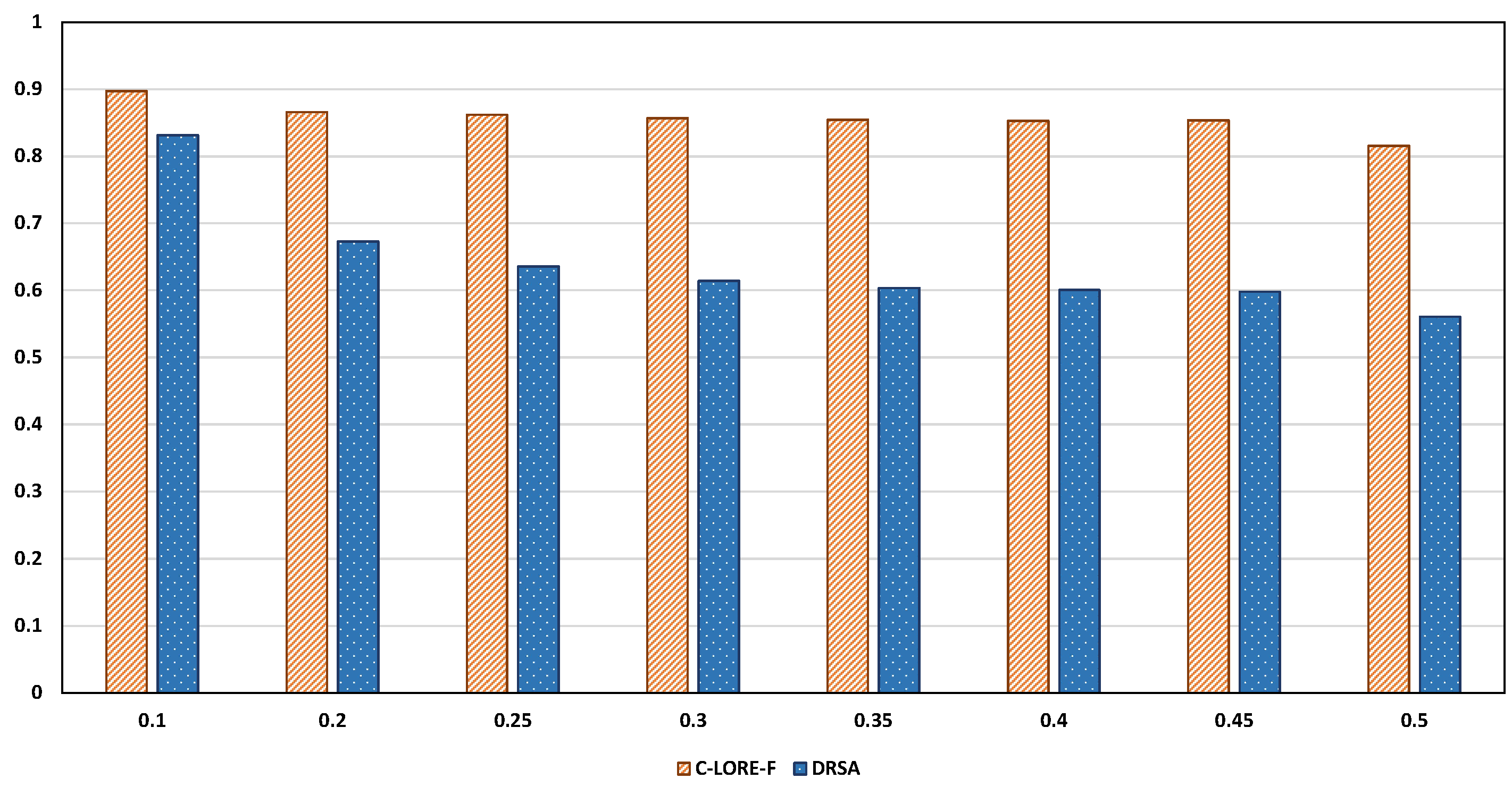
5.3. Evaluating the Locality of the Methods

The proposed explanation system is local, because it focuses on the behaviour of RETIPROGRAM around the specific instance x. The Fidelity metrics defined above validate the models’ performance in terms of locality with respect to the generated neighbours and the instance to be explained. Assuming that we have access to the test set used to evaluate the black-box model, we can validate the locality of the model with respect to the test set by defining a new metric, the xt-Fidelity. It is the fidelity measure computed on the set of instances from the test set with a distance to the instance x less than or equal a threshold t. The overall xt-Fidelity on a set X given a threshold t is computed by taking the average of xt-Fidelity for all $x\in X$. We use it to measure the locality vs the globality of the explanation method. It is expected that a local method shows a degradation in its performance with large thresholds, as a significant number of the selected instances will belong to subspaces different than the one used to build the explanation model.

We compared the xt-Fidelity results of both C-LORE-F and DRSA under different thresholds as illustrated in Figure 4. In general, we can find that, as the threshold increases, the overall score decreases, which means we lose the models’ locality. In other words, the input space turns out to be more global, and the model fails to cover that space. The degradation in the performance is obvious in the case of DRSA. On the other hand, the C-LORE-F method mostly preserves the performance (the degradation is minor than in DRSA). We can attribute that to the fact that the multiple and small decision trees of C-LORE-F were trained on subspaces of the global space and formed a random forest model. Such a model can show comparable performance on the test set to the performance of RETIPROGRAM (a fuzzy random forest model built from multiple fuzzy decision trees). Hence, if the locality of the explanation model is more important than the globality, we can choose DRSA. Otherwise, C-LORE-F is ideal.

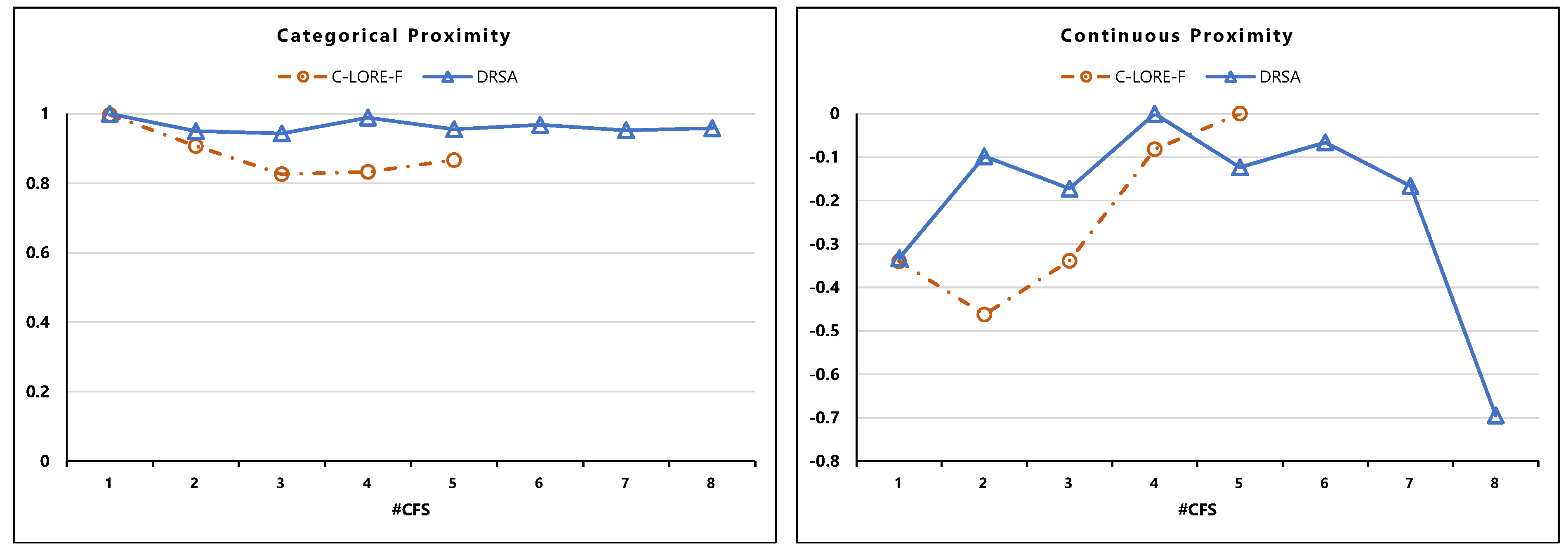
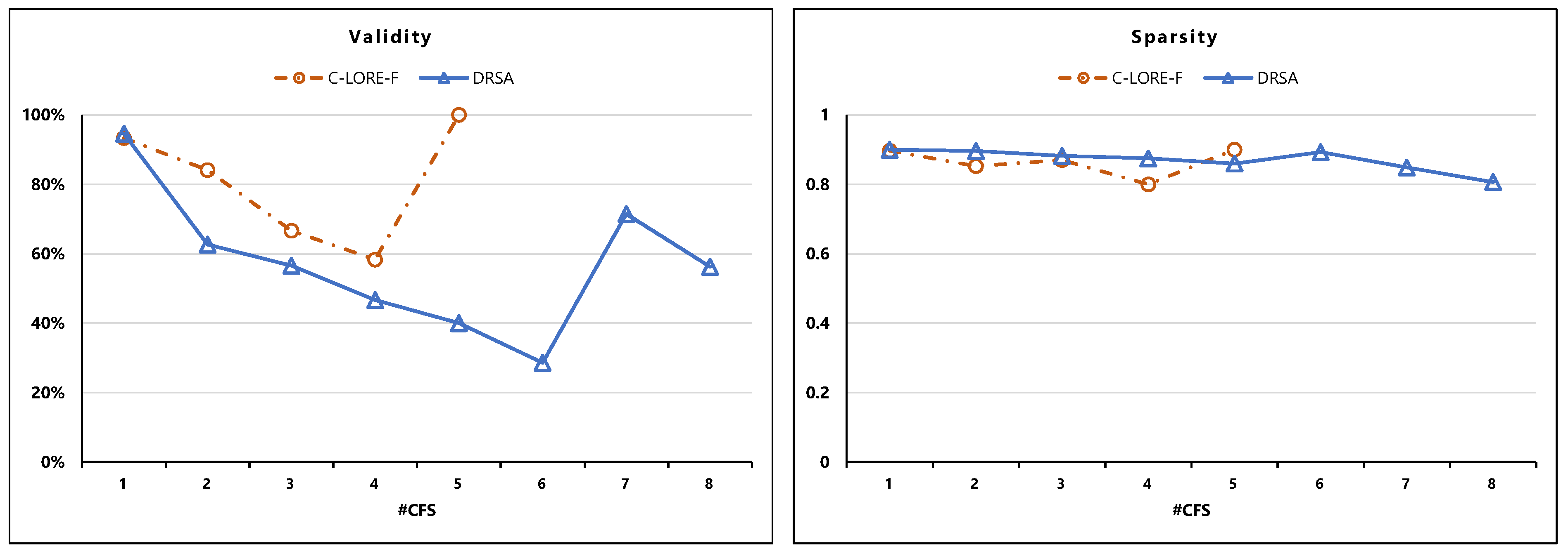
5.4. Evaluation of the Counterfactual Examples

It is well-known that counterfactual examples help to understand what changes are needed to obtain a different outcome. This is particularly interesting in health-care applications. Hence, it is important to have counterfactual examples that balance a wide range of suggested modifications (diversity) and the relative facility of adopting those modifications (proximity to the actual input). Moreover, counterfactual examples must be actionable, e.g., people can not reduce their age or change their race.

In this subsection, we evaluate the generated counterfactual examples using the following evaluation metrics [22]:

• Validity: is the number of counterfactual examples with a different outcome than the original input, i.e., x, divided by the total number of counterfactual examples.

  $$\mathrm{Validity}=\frac{|\widehat{x}\in \mathbb{C}s.t.b\left(x\right)\ne b\left(\widehat{x}\right)|}{\left|\mathbb{C}\right|}$$

  (1)
  Here $\mathbb{C}$ refers to the set of returned counterfactual examples and b is the black-box model.
• Proximity: is the mean of feature-wise distances between a counterfactual example c and the original input x. We considered two different proximity measures, the Euclidean distance for the continuous features and the Hamming distance for the categorical ones.

  $$\mathrm{Continuous}\mathrm{Proximity}=-\frac{1}{\left|\mathbb{C}\right|}\sum _{c\in \mathbb{C}}dist\_cont(c,x)$$

  (2)

  $$\mathrm{Categorical}\mathrm{Proximity}=1-\frac{1}{\left|\mathbb{C}\right|}\sum _{c\in \mathbb{C}}dist\_cat(c,x)$$

  (3)
• Sparsity: it measures the average of changes between a counterfactual example and the original input.

  $$\mathrm{Sparsity}=1-\frac{1}{\left|\mathbb{C}\right|*\left|\mathbb{F}\right|}\sum _{c\in \mathbb{C}}\sum _{f\in \mathbb{F}}\mathbb{1}[c_f\ne x_f]$$

  (4)
  Here, $\mathbb{F}$ is the set of features, and $\mathbb{1}$ is the indicator function.
• Diversity: it is similar to proximity. However, instead of computing the feature-wise distance between the counterfactual example and the original input, we compute it between each pair of counterfactual examples. As in the proximity measure, we considered two different diversity versions, one for the continuous and the other for the categorical features.

Figure 5 shows the results of the Validity and Sparsity metrics for C-LORE-F and DRSA. C-LORE-F generates better valid counterfactual examples than DRSA. For both of them, when they generate a single counterfactual example, it is valid (near 100%). Notice that C-LORE-F has never generated more than 5 counterfactual examples. On the contrary, DRSA is able to generate more counterfactuals but the validity decreases and sparsity keeps similar.

Both C-LORE-F and DRSA show outstanding performance on Sparsity (DRSA is slightly better) with an average of 0.9.

Looking at the Diversity results (Figure 6), we can find that C-LORE-F generates more diverse examples with respect to the categorical features and diversity increases as the number of counterfactual examples increases. In the case of continuous features, DRSA is slightly better than C-LORE-F.

The Proximity results are shown in Figure 7. C-LORE-F generates counterfactual examples with lower proximity than DRSA for both the categorical and continuous features. Moreover, the inherent trade-off between diversity and proximity metrics can be observed in the case of categorical features.

5.5. Analysis of Computational Complexity

Computational resources are crucial in any practical application. In this subsection, we analyse the time complexity of the system. The most costly parts of the system are the generation of neighbours, the construction of the decision tree and the construction of the rules in the DRSA method. So, we first present the theoretical analysis of the time complexity of each part, and then we show the experimental setup and the running time in seconds.

We solve the generation of neighbours as a searching problem using the Uniform Cost Search algorithm. Hence, the total running time complexity of this part of the system is $O\left(b^{1+\lfloor C^{*}/ϵ\rfloor }\right)$, where b is the branching factor and $C^{*}$ is the cost of the optimal solution, assuming that every action costs at least $ϵ$ [34]. The time complexity for the decision tree algorithm is $O\left(n\right)+O(m·n·lo{g}_{2}n)+O(n·lo{g}_{2}n)$ [35]. The time complexity of the DRSA method is $O(m^2·n^2)$. Here, m is the number of examples, and n is the number of attributes.

The experiments were carried out on a 64- bit computer, with AMD Ryzen 7 3700U (4 Cores, 2.3 GHz) and 16 GB RAM, running Windows 11 operating system. The number of examples in the test set is 1111. For each example, we generate 800 neighbours and use them to derive the explanation.

Table 3. Running time comparisons.

	Min	Max	Average
Neighbours Generation	5.453	19.252	8.882
C-LORE-F	0.093	1.149	0.169
DRSA	0.125	2.556	0.386

shows the elapsed time of generating the neighbours, building the decision trees and constructing the rules in seconds. As expected, the most expensive part of the system is the generation of the neighbours. The decision tree is slightly faster than the DRSA, which is expected as the DRSA complexity is quadratic, whereas the decision tree complexity is logarithmic. The estimated time to obtain an explanation is 9.051 s using the C-LORE-F method and 9.268 s using the DRSA method.

6. Conclusions

We have proposed a methodology to derive an explanation for the decision made by the RETIPROGRAM system, which was developed in our research group to estimate the personalised risk of developing diabetic retinopathy as early as possible. RETIPROGRAM is in use at a regional hospital in city of Reus (Spain). The paper is focused on comparing two different explanation methods: one based on decision trees (C-LORE-F) and the other one based on decision rules (DRSA). These methods are post-hoc explanation methods and rely on the generation of neighbours around the instance to be explained, which are used to train an explainable model (either a decision tree or decision rules), and finally they generate an explanation from that local model. The explanation result is formed by the rule(s) applicable to the instance, a set of counterfactual rules and a set of counterfactual instances. C-LORE-F with DT was previously published in [13], where was compared with other state of the art methods. The current paper shows that DRSA is also a valid method for generating explanatory rules. After comparing the obtained explanation from the C-LORE-F and DRSA methods using multiple evaluation metrics, we found that both of them generate an adequate explanation. C-LORE-F is slightly better in hid and fidelity indicators, but its sparsity is a bit smaller than the one of DRSA. We have also shown that the time needed for the generation of the explanation is of 9 s, which is an acceptable time for real use for medical physicians when visiting a patient.

As a weak point, we found that the counterfactual instances are not sufficiently good. In our future work, we will focus on resolving this issue by improving the generation of counterfactual examples [22].

It is worth to mention that the methods proposed for constructing explanations based on rules are general even if they have been studied for the Diabetic Retinopathy problem. They could be applied to other fields and with any other black box classifier.

References

1. Aguiree, F.; Brown, A.; Cho, N.H.; Dahlquist, G.; Dodd, S.; Dunning, T.; Hirst, M.; Hwang, C.; Magliano, D.; Patterson, C.; et al. IDF Diabetes Atlas; International Diabetes Federation: Brussels, Belgium, 2013. [Google Scholar]
2. Shaw, J.E.; Sicree, R.A.; Zimmet, P.Z. Global estimates of the prevalence of diabetes for 2010 and 2030. Diabetes Res. Clin. Pract. 2010, 87, 4–14. [Google Scholar] [CrossRef] [PubMed]
3. Nair, A.T.; Muthuvel, K.; Haritha, K. Effectual Evaluation on Diabetic Retinopathy. In Information and Communication Technology for Competitive Strategies (ICTCS 2020); Springer: Singapore, 2022; pp. 559–567. [Google Scholar]
4. López, M.; Cos, F.X.; Álvarez-Guisasola, F.; Fuster, E. Prevalence of diabetic retinopathy and its relationship with glomerular filtration rate and other risk factors in patients with type 2 diabetes mellitus in Spain. DM2 HOPE study. J. Clin. Transl. Endocrinol. 2017, 9, 61–65. [Google Scholar] [CrossRef] [PubMed]
5. Romero-Aroca, P.; Valls, A.; Moreno, A.; Sagarra-Alamo, R.; Basora-Gallisa, J.; Saleh, E.; Baget-Bernaldiz, M.; Puig, D. A clinical decision support system for diabetic retinopathy screening: Creating a clinical support application. Telemed. e-Health 2019, 25, 31–40. [Google Scholar] [CrossRef] [PubMed] [Green Version]
6. Saleh, E.; Valls, A.; Moreno, A.; Romero-Aroca, P.; Torra, V.; Bustince, H. Learning fuzzy measures for aggregation in fuzzy rule-based models. In International Conference on Modeling Decisions for Artificial Intelligence; Springer: Cham, Switzerland, 2018; pp. 114–127. [Google Scholar]
7. Romero-Aroca, P.; Verges-Pujol, R.; Santos-Blanco, E.; Maarof, N.; Valls, A.; Mundet, X.; Moreno, A.; Galindo, L.; Baget-Bernaldiz, M. Validation of a diagnostic support system for diabetic retinopathy based on clinical parameters. Transl. Vis. Sci. Technol. 2021, 10, 17. [Google Scholar] [CrossRef] [PubMed]
8. Burkart, N.; Huber, M.F. A Survey on the Explainability of Supervised Machine Learning. J. Artif. Intell. Res. 2021, 70, 245–317. [Google Scholar] [CrossRef]
9. Strumbelj, E.; Kononenko, I. An efficient explanation of individual classifications using game theory. J. Mach. Learn. Res. 2010, 11, 1–18. [Google Scholar]
10. Krause, J.; Perer, A.; Ng, K. Interacting with predictions: Visual inspection of black-box machine learning models. In Proceedings of the 2016 CHI Conference on Human Factors in Computing Systems, San Jose, CA, USA, 7–12 May 2016; pp. 5686–5697. [Google Scholar]
11. Ribeiro, M.T.; Singh, S.; Guestrin, C. Why Should I Trust You?: Explaining the Predictions of Any Classifier. In Proceedings of the 22nd ACM SIGKDD International Conference on Knowledge Discovery and Data Mining, San Francisco, CA, USA, 13–17 August 2016; pp. 1135–1144. [Google Scholar]
12. Maaroof, N.; Moreno, A.; Valls, A.; Jabreel, M. Guided-LORE: Improving LORE with a Focused Search of Neighbours. In International Workshop on the Foundations of Trustworthy AI Integrating Learning, Optimization and Reasoning; Springer: Cham, Switzerland, 2020; pp. 49–62. [Google Scholar]
13. Maaroof, N.; Moreno, A.; Jabreel, M.; Valls, A. Contextualized LORE for Fuzzy Attributes. In Artificial Intelligence Research and Development; IOS Press: Amsterdam, The Netherlands, 2021; pp. 435–444. [Google Scholar]
14. Saleh, E.; Moreno, A.; Valls, A.; Romero-Aroca, P.; de La Riva-Fernandez, S. A Fuzzy Random Forest Approach for the Detection of Diabetic Retinopathy on Electronic Health Record Data. In Artificial Intelligence Research and Development; Frontiers in Artificial Intelligence and Applications; IOS Press: Amsterdam, The Netherlands, 2016; Volume 288, pp. 169–174. [Google Scholar]
15. Greco, S.; Matarazzo, B.; Slowinski, R. Rough sets theory for multicriteria decision analysis. Eur. J. Oper. Res. 2001, 129, 1–47. [Google Scholar] [CrossRef]
16. Guidotti, R.; Monreale, A.; Ruggieri, S.; Turini, F.; Giannotti, F.; Pedreschi, D. A survey of methods for explaining black box models. ACM Comput. Surv. 2018, 51, 1–42. [Google Scholar] [CrossRef] [Green Version]
17. Molnar, C. Interpretable Machine Learning; Lulu.com: Morrisville, NC, USA, 2020. [Google Scholar]
18. Ribeiro, M.T.; Singh, S.; Guestrin, C. Anchors: High-Precision Model-Agnostic Explanations. AAAI 2018, 18, 1527–1535. [Google Scholar]
19. Lundberg, S.M.; Lee, S.I. A unified approach to interpreting model predictions. Adv. Neural Inf. Process. Syst. 2017, 30, 4765–4774. [Google Scholar]
20. Martens, D.; Provost, F. Explaining data-driven document classifications. MIS Q. 2014, 38, 73–100. [Google Scholar] [CrossRef]
21. Guidotti, R.; Monreale, A.; Ruggieri, S.; Pedreschi, D.; Turini, F.; Giannotti, F. Local rule-based explanations of black box decision systems. arXiv 2018, arXiv:1805.10820. [Google Scholar]
22. Mothilal, R.K.; Sharma, A.; Tan, C. Explaining machine learning classifiers through diverse counterfactual explanations. In Proceedings of the 2020 Conference on Fairness, Accountability, and Transparency, Barcelona, Spain, 27–30 January 2020; pp. 607–617. [Google Scholar]
23. Russell, C. Efficient search for diverse coherent explanations. In Proceedings of the Conference on Fairness, Accountability, and Transparency, Atlanta, GA, USA, 19–31 January 2019; pp. 20–28. [Google Scholar]
24. Ming, Y.; Qu, H.; Bertini, E. Rulematrix: Visualizing and understanding classifiers with rules. IEEE Trans. Vis. Comput. Graph. 2018, 25, 342–352. [Google Scholar] [CrossRef] [Green Version]
25. Neto, M.P.; Paulovich, F.V. Explainable Matrix—Visualization for Global and Local Interpretability of Random Forest Classification Ensembles. IEEE Trans. Vis. Comput. Graph. 2020, 27, 1427–1437. [Google Scholar] [CrossRef] [PubMed]
26. Wilson, D.R.; Martinez, T.R. Improved heterogeneous distance functions. J. Artif. Intell. Res. 1997, 6, 1–34. [Google Scholar] [CrossRef]
27. Ruggieri, S. YaDT: Yet another Decision Tree Builder. In Proceedings of the 16th IEEE International Conference on Tools with Artificial Intelligence (ICTAI 2004), Boca Raton, FL, USA, 15–17 November 2004; pp. 260–265. [Google Scholar]
28. Pawlak, Z. Rough Sets: Theoretical Aspects of Reasoning about Data; Springer Science & Business Media: Dordrecht, The Netherlands, 1991; Volume 9. [Google Scholar]
29. Słowiński, R.; Greco, S.; Matarazzo, B. Rough set methodology for decision aiding. In Springer Handbook of Computational Intelligence; Springer: Berlin/Heidelberg, Germany, 2015; pp. 349–370. [Google Scholar]
30. Błaszczyński, J.; Słowiński, R.; Szeląg, M. Sequential covering rule induction algorithm for variable consistency rough set approaches. Inf. Sci. 2011, 181, 987–1002. [Google Scholar] [CrossRef]
31. Błaszczyński, J.; Słowiński, R.; Szeląg, M. Induction of Ordinal Classification Rules from Incomplete Data. In Rough Sets and Current Trends in Computing; Yao, J., Yang, Y., Słowiński, R., Greco, S., Li, X., Mitra, S., Polkowski, L., Eds.; Springer: Berlin/Heidelberg, Germany, 2012; Volume 7413, pp. 56–65. [Google Scholar]
32. Saleh, E.; Maaroof, N.; Jabreel, M. The deployment of a decision support system for the diagnosis of Diabetic Retinopathy into a Catalan medical center. In Proceedings of the 6th URV Doctoral Workshop in Computer Science and Mathematics; Universitat Rovira i Virgili: Tarragona, Spain, 2020; p. 45. [Google Scholar]
33. Blanco, M.E.S.; Romero-Aroca, P.; Pujol, R.V.; Valls, A.; SaLeh, E.; Moreno, A.; Basora, J.; Sagarra, R. A Clinical Decision Support System (CDSS) for diabetic retinopathy screening. Creating a clinical support application. Investig. Ophthalmol. Vis. Sci. 2020, 61, 3308. [Google Scholar]
34. Russell, S.; Norvig, P. Artificial Intelligence: A Modern Approach, 4th ed.; Pearson: London, UK, 2020. [Google Scholar]
35. Sani, H.M.; Lei, C.; Neagu, D. Computational complexity analysis of decision tree algorithms. In International Conference on Innovative Techniques and Applications of Artificial Intelligence; Springer: Cham, Switzerland, 2018; pp. 191–197. [Google Scholar]
Figure 1. Illustration of the next and prev actions.
Applsci 12 03358 g001
Figure 2. Architecture of the proposed explanation generation methodology.
Applsci 12 03358 g002
Figure 3. The constructed rules using the explanation system for x.
Applsci 12 03358 g003
Figure 4. Degree of locality vs globality of the explanation models. The x-axis represents the thresholds and the y-axis represents the xt-Fidelity.
Applsci 12 03358 g004
Figure 5. Validity and Sparsity of counterfactual examples. The numbers in the y-axis represent the metrics values (the higher values the better performance), while the x-axis represents the number of generated counterfactual instances.
Applsci 12 03358 g005
Figure 6. Diversity of counterfactual examples, in Categorical and Continuous attributes. The numbers in the y-axis represent the metrics values (the higher values the better performance), while the x-axis represents the number of generated counterfactual instances.
Applsci 12 03358 g006
Figure 7. Proximity of counterfactual examples, in Categorical and Continuous attributes. The numbers in the y-axis represent the metrics values (the higher values, the better performance), while the x-axis represents the number of generated counterfactual instances.
Applsci 12 03358 g007