
Analytical Solution and Shaking Table Test on Tunnels through Soft-Hard Stratum with a Transition Tunnel and Flexible Joints


1
Key Laboratory of Urban Underground Engineering of Ministry of Education, Beijing Jiaotong University, Beijing 100044, China
2
School of Civil Engineering, Beijing Jiaotong University, Beijing 100044, China
*
Author to whom correspondence should be addressed.
Appl. Sci. 2022, 12(6), 3151; https://doi.org/10.3390/app12063151
Submission received: 11 January 2022
/
Revised: 8 March 2022
/
Accepted: 13 March 2022
/
Published: 19 March 2022
(This article belongs to the Special Issue Tunneling and Underground Engineering: From Theories to Practices)
Abstract
:Tunnels, where they pass through soft-hard strata, are severely damaged during earthquakes. These issues have not yet been well understood. In this study, the seismic performances of a tunnel passing through soft-hard stratum with a transition tunnel and flexible joints under earthquake motion were investigated by proposed analytical solutions and scaled shaking table tests. First, a mechanical model of a tunnel passing through soft-hard stratum with flexible joints is proposed, and it is derived by the Green’s function method. Then, a parametric analysis is conducted to investigate the effects of important variables on tunnels through soft-hard stratum. Finally, shaking table tests are conducted to verify the proposed solution and further investigate the seismic behaviors of the tunnel. The results show that: (1) the analytical solutions are workable and effective; (2) the influence of the soft-hard stratum junction on the tunnel responses is remarkable—the largest bending moment is located at the side of soft rock near the sharp contact area and the maximum shear force appears at the contact; (3) the joints and the transition tunnel could mitigate the potential adverse effects of the sharp contact area—the region affected by the joint is approximately 4.5 times the tunnel diameter on both sides of the stratum interface; and (4) the influence of sharp change of ground layers is more remarkable with a larger excitation amplitude.
1. Introduction
In recent years, with the rapid development in China, the national high-speed railway network extends to the northwest and southwest mountainous areas, which are high-intensity earthquake zones. These areas contain many problematic areas including complicated formations, severely tectonized and faulted zones, and so on. Therefore, tunnels, as a major part of civil infrastructures, are likely to pass through soft-hard strata. Many post-earthquake investigations have shown that the tunnel section at the junction of the soft and hard rock is severely damaged [1,2,3]. Therefore, tunnels through soft-hard strata should be paid much attention.
There are an increasing number of studies on dynamic responses of tunnel structures passing through soft-hard strata. Liang et al. [4] conducted a series of shaking table tests and numerical simulations to investigate the dynamic responses of a shield tunnel passing through a soft-hard stratum. The results showed that the strain of the tunnel around the soft-hard interface increased significantly. Koizumi and He [5] showed that a secondary lining had a significant impact on responses of the segments under longitudinal excitation rather than transverse excitation using shaking table tests. Zhang et al. [6] found that the acceleration responses for the soft-hard junction stratum exhibited double predominant frequency by model tests and numerical simulations. Wang et al. [7] proved that the seismic damage of tunnel was mainly caused by the forced displacement under the condition of interface between soft and hard rock through shaking table tests. Tang et al. [8] investigated the seismic responses of a utility tunnel, and the results showed that a sharp variation of response occurred at the interface between soft soil and hard soil, and that the variation under a far-field earthquake could be more significant.
In terms of theoretical calculations, two kinds of approaches have been developed to study the longitudinal response of tunnel structures, namely the free field deformation approach and the soil-structure interaction approach [9,10]. The first method involves the strains and deformations of tunnel structure being obtained by imposing free-field deformations on the structure [11]. However, the method always overestimates or underestimates the structure deformations due to neglect of interaction between the tunnel and surrounding ground [12,13,14]. For the soil-structure interaction approach, the beam-on-elastic foundation approach is used to model soil-structure interaction effects [15]. Tariverdilo et al. [16] proposed a mathematical model for analyzing the effect of submergence on the dynamic response of submerged floating tunnel due to moving load. Yu et al. presented an analytical solution for the responses of tunnel liners crossing through soil-rock stratum based on the Euler–Bernoulli beam on elastic foundation approach [17,18,19]. The present approach mainly relies on the assumption that the surrounding rock is homogeneous, that is to say no sharp change of properties in surrounding rock along the tunnel.
The transition of stiffness of the liner, e.g., over-excavation, lining thickening, or both, is often performed, and flexible connections between the transition segments and adjacent segments are also suggested in practice to mitigate effects of a sharp change when tunnels run through soft-hard junction stratum. However, little research can be found in literature on this problem.
In this paper, seismic performances of a tunnel passing through soft-hard stratum equipped with a transition tunnel and flexible joints under earthquake motion were investigated by a new proposed simplified analytical solution and a series of scaled shaking table tests. First, a mechanical model of a tunnel passing through soft-hard stratum with flexible joints was proposed and the longitudinal seismic responses of the tunnel was derived by the Green’s function method. Then, a parametric analysis was performed to investigate the effects of important variables on tunnels through soft-hard stratum and the influence of joint and the optimal length of transition zone were discussed. Finally, shaking table tests were conducted to verify the proposed solution and further investigate the seismic behaviors of the tunnel.
2. Simplified Analytical Solution
In this section, a simplified analytical solution is developed to evaluate the responses of a tunnel with flexible joints through a soft-hard stratum junction under earthquake motion, as shown in Figure 1. A tunnel with three regions is designed where the two regions on the right side are thickened, which is often adopted for the sudden change in rock type and soft rock. In addition, the flexible connection is set between the regions. The transition Region 2 consists of two segments and the flexible connection is also set between them, which is intended to mitigate the influence of the sharp change in properties of the surrounding rock on the tunnel responses. The other two regions, which consist of one segment each, are embedded in hard layer (Rock 1) and soft layer (Rock 2), respectively. Note that Rock 1 is harder than Rock 2. To simplify the problem, the tunnel is assumed to behave as a shear beam on viscoelastic foundation. The following assumptions are made:
- Each lining segment has homogeneous isotropic linear elasticity and its sounding rock is viscoelastic.
- The axial deformation of the tunnel is not considered.
- The seismic input motion is assumed as an incident sinusoidal wave.
Considering an idealized model of a tunnel with flexible joints, a mechanical model shown in Figure 2 is built. In the model, a mechanical model of shear spring and rotation spring is assumed to model the flexible joint between lining segments, which considers the differences of both displacement and rotation angle, as suggested by Ref [9,20]. This can accommodate the movement caused by non-homogeneous ground. Cwk and CΦk are the stiffness coefficients of extensional spring and rotational spring, respectively. Three joints were designed and denoted as Joint 1, Joint 2, and Joint 3. The lining segments are supported by foundations with different spring coefficients K1 and K2 and different damping coefficients c1 and c2, respectively. The stiffness and mass per unit length of the lining segment are EIj and ρAj (j = 1,2,3,4), respectively, where E is the Young’s modulus of elasticity, Ij and Aj are the moment of inertia and area of the cross section, respectively, and ρ is the density of the lining. For the sake of simplicity, the transverse shear wave is considered here. The transverse displacements of the free field under sinusoidal shear motions, which is propagating parallel to the tunnel axis, is defined as wg (x,t). wg is expressed as:
where wmax1(wmax2) is the peak free field transverse displacement in Rock 1 (Rock 2), which can be obtained by a design response spectrum or site response analysis techniques [19], e.g., DEEPSOIL [21]; λ1 and λ2 are the wavelength of the transverse motions in hard and soft layers, respectively; θ is the incident angle earthquake wave; and α0 is the displacement phase angle.
2.1. Closed-Form Solution for Responses of Tunnel Lining under Earthquake Wave
Using the Hamilton principle and employing the shear beam theory, the governing equation of the tunnel is given by [22,23]:
where φ is the bending angle; κ is the shear correction coefficient; G is the shear modulus; μ = ρA and γ = ρI represent the mass and the rotation inertia of the beam per unit length, respectively; K and c are the foundation modulus and damping coefficient, respectively; the prime indicates a derivative with respect to the spatial coordinate x; and the dot stands for a derivative with respect to time.
In the case where the load is a harmonic load wg(x,t) = Wg(x)∙eiΩt, the displacement and the rotation angle can be also expressed as w(x,t) = W(x)∙eiΩt and φ(x,t) = Φ(x)∙eiΩt, respectively. Inserting those expressions in Equation (1) will eliminate the time variable, and the equation will be recast to:
where i is the imaginary unit, Ω is loading frequency, and t is time.
From Equation (3), it can be simplified to:
Then it can be symbolically presented as:
where
By means of the superposition principle, the solution of Equation (5) can be input in the following form [24]:
where G(x, x0) is the Green’s function to be determined. G(x, x0) is the deflection of the tunnel at point x due to a unit concentrated load acting at an arbitrary position x = x0. Mathematically, G(x, x0) is the solution of the following equation:
Though Laplace transform and Laplace inverse transform, Equation (8) will lead to the explicit expression of the Green’s function G(x, x0):
where H(∙) is the Heaviside function, and W(0), W′(0), W″(0), W‴(0) are the constants, which are determined by the boundary conditions of the tunnel.
The expressions of ϕ1, ϕ2, ϕ3, ϕ4 and ϕ5 are:
where
The symbols sl(l = 1,2,3,4) are roots of the following equation:
Therefore, the displacement can be obtained by Equation (7). Subsequently, the rotation angle, bending moment and shear force along the tunnel are obtained from the expressions below:
2.2. Closed-Form Solution of Tunnel through Soft-Hard Stratum Junction with Flexible Joints
In this section, the analytical solution to the problem in Figure 2 is developed. Four lining segments in Figure 2 are considered. For the sake of solution, the deformation of each part is separately studied, and local coordinate systems O1–x1y1, O2–x2y2, O3–x3y3 and O4–x4y4 are built, as shown in Figure 2. Hence, the expression of the Green’s functions G(x, x0) of the model appears as a four-step piecewise function. The free boundaries are applied in the mechanical model, as presented by Yu et al. [25], so the Green’s functions of the beams are:
where and .
Due to the existence of joints, the discontinuous displacement and rotation angle at joint can be written as:
at joint k(k = 1,2),
Substituting Equation (16) into Equation (17), the following relation can be obtained:
where Uk = (Ak, Bk, Ck, Dk)T, Uk+1 = (Ak+1, Bk+1, Ck+1, Dk+1)T, and other parameters in Equation (18) are given in Appendix A.
The continuity conditions at the joint k = 3 are different from those of other joints due to the difference between its local coordinate and others, and it can be expressed as:
Substituting Equation (16) into Equation (19), the following equation is obtained:
where U3 = (A3, B3, C3, D3)T, U4 = (A4, B4, C4, D4)T, and other parameters in Equation (20) are given in Appendix A.
The unascertained coefficients can be calculated via Equations (18) and (20). Then, inserting these coefficients into Equation (16), the Green’s functions in the local coordinate systems can be obtained. Subsequently, the Green’s functions in the global coordinate systems can be expressed as:
Thus, the responses of the tunnel through soft-hard stratum junction equipped with flexible joints can be obtained by Equation (7) and Equations (13)–(15).
3. Analytical Results
3.1. Project Introduction
Located in western Sichuan province, China, a shallow-buried tunnel through soft-hard stratum junction is considered in this paper. The rock mass along the tunnel is organized into two classes with grade IV and VI (the rock is worse with growing grade numbers) according to the Chinese Code for Design of Road Tunnel (JGJ 70-2004). In order to reduce the influence of the sharp change of ground properties on the tunnel responses, the transition zone and flexible connections were suggested to be adopted for the project. Note that the positions of Joint 1, Joint 2 and Joint 3 are located between Region 1 and Region 2, between the hard layer and soft layer, and between Region 2 and Region 3, correspondingly. In light of on-site geologic investigation of the tunnel, the shear velocities of the hard layer (Rock 1) and the soft layer (Rock 2) are 687 m/s and 430 m/s, respectively. The spring constants of foundation are K1 = 0.63 GPa in Rock 1 and K2 = 0.36 GPa in Rock 2, which are obtained using following equation [15]:
where ρ and ν are density and Poisson’s ratio of soil, respectively, vs. is shear velocity, d is the diameter of a tunnel, and λ is wavelength.
In addition, the density and Poisson’s ratio of the Rock 1 are 2200 kg/m3 and 0.3, respectively. The density and Poisson’s ratio of the Rock 2 are 1800 kg/m3 and 0.35, correspondingly. The tunnel is subjected to a sinusoidal shear motion with wavelength λ1 = 344 m in Rock 1 and λ2 = 215 m in Rock 2. Note that the seismic input motion is assumed as an incident sinusoidal wave. The East-West(EW) component of seismic waves in Mao County is imposed at the bottom of the surrounding rock, and the peak ground acceleration is 0.4 g (g is the gravitational acceleration), as shown in Figure 3. The maximum free transverse displacement in Rock 1 is umax1 = 0.017 m, and the maximum displacement in Rock 2 is umax2 = 0.029 m, which were analyzed from DEEPSOIL. The cross sections of the tunnel segments are nearly circular. The outer diameter of segment 1 is 10.8 m and the outer diameter of the rest of the segments is 11.4 m, which are determined by equivalent area. The inner diameter of all the segments is 9.6 m. The moment of inertia of segment 1 is 242 m4, and the moment of inertia of segment 2, segment 3 and segment 4 is the same, with 398 m4. The Young’s modulus and the shear correction coefficient of tunnel are E = 30 GPa and κ = 0.52, respectively.
3.2. General Responses
To investigate the influences of the soft-hard stratum junction on the tunnel responses, three cases are considered: (1) a uniform tunnel crossing soft-hard stratum junction; (2) a uniform tunnel buried in uniform hard layer with spring constants of foundation K1 = K2 = 0.63 GPa and wavelength λ1 = λ2 = 344 m; and (3) a uniform tunnel buried in uniform soft layer with spring constants of foundation K1 = K2 = 0.36 GPa and wavelength λ1 = λ2 = 215 m. The stiffness of the uniform tunnel is constant with 7.53 × 10¹² N·m2, and no damping and no flexible joints are adopted for all three cases. Other parameters are same as those introduced in Section 4.1.
Figure 4 shows the internal force responses of a uniform tunnel across a soft-hard stratum junction (Case 1). As it can be seen, two peak bending moments occur near sharp contact, which means the sudden change of the ground layers leads to significant bending moments in the contact area of non-homogeneous layers. This phenomenon is in agreement with the finding from [19]. It is interesting to see that the largest bending moment is located at the side of soft layer near the sharp contact area, which is accordance with shaking table test results [6]. To put it another way, the most unfavorable location of the bending moment is determined by the combination of the sharp contact and the weak surrounding rock, which is the key position for aseismic design. Figure 4 shows that the maximum shear force appears at contact, and the farther from the contact, the smaller the shear force. Compared to the analytical solution and the existing research, the longitudinal responses have a lot in common, showing that the closed-form analytical solutions are accurate.
In order to better describe the influence of sharp change of ground layers on the seismic response of the tunnel structure, the results of case 1 are normalized, where the normalized values are calculated with respect to those of case 2 in the hard layer and the normalized values are calculated with respect to those of case 3 in the soft layer. It can be clearly seen from Figure 5 that the internal forces are obviously amplified around the soft-hard interface. At the same time, the maximum internal force amplification factors occur in the range of about 1 D (D is the outer diameter of the tunnel). In terms of moment, the maximum amplified factor occurs in the hard layer near the interface along the tunnel axis, which indicates that the tunnel in the hard layer should also be adopted for anti-seismic measures when a tunnel passes through a soft-hard stratum. Therefore, the transition zone in relatively hard rock is needed as well. There are two peak amplified factors of shear force appearing near the interface where the largest one is located in the soft rock near the interface, as shown in Figure 5b. Above all, the influence of the soft-hard stratum junction on the tunnel responses is remarkable. The maximum amplified factor is in relatively hard rock for the bending moment, and is in soft rock for the shear force.
3.3. Influence of Joint on Responses of Tunnel
This section investigates the influence of the joint on the responses of the tunnel built in non-homogeneous ground. The parameters introduced in Section 4.1 are also employed here. For the sake of convenience in the study, the following dimensionless variables ζwk = Cwk/κGA, ζΦk = CΦk/EI are introduced, and the parameters of the joints are set as ζwk = 0.05, ζΦk = 0.05, as suggested in Ref [26].
Figure 6 shows the displacements of tunnels with and without joints along the tunnel axis. As it can be seen, the displacement difference at Joint 2 is the largest, which indicates that the sharp change of ground layers has a great influence on displacement of the tunnel, and that the flexible joint works.
Figure 7 illustrates the internal force responses of tunnels with and without joints. The laws of the tunnel internal forces are similar with those in Section 4.2 in spite of different stiffnesses of tunnels, which verifies that the tunnel responses are mainly affected by surrounding rocks. It shows that the joints efficiently reduce bending moments and shear forces of the tunnel. For example, the maximum bending moment of the lining with a joint is 43.75% less than that without a joint, and the maximum shear force with a joint is reduced by 30.89% compared with that without joints. Moreover, the region affected by the joint is approximately 4.5 times the tunnel outer diameter on both sides of the stratum interface.
3.4. Influence of the Length of the Transition Zone
In practice, a transition tunnel is often included to mitigate the potential adverse effects of the sharp change of ground properties. To investigate the effect of the length of the transition zone, four cases with different length of the transition zone are investigated, with values of 0 m, 24 m, 48 m and 96 m, considering that the length of the concrete trolley in tunnel construction is generally 9 m or 12 m at present. Note that 0 m indicates that no Region 2 is considered. Figure 8 shows the maximum bending moment and shear force of the tunnel structure under the different scenarios discussed. The minimum value of bending moment occurs when the length of Region 2 is 36 m, followed by the length of Region 2 being 24 m and 48 m, where the maximum bending moments are very close to each other. In terms of the shear force, the Region 2 of 24 m has the minimum value, and the one with 36 m is 2.55% larger than that with 24 m. Therefore, the length of Region 2 with 24 m or 36 m can be taken as the optimal length.
4. Shaking Table Test
The model test is the most direct method to study the response characteristics of tunnel structures, and also the basis of numerical simulation and theoretical analysis [27,28]. In this paper, experimental model tests were used to verify the analytical solution to ensure that they could reveal reasonable predictions.
4.1. Test Modelling and Apparatus
Taking the shallow-buried tunnel through soft-hard stratum junction as a prototype and inputting the seismic wave recorded in the Wenchuan earthquake, the shaking table tests were conducted to research the dynamic response of a tunnel passing through soft-hard stratum. The longitudinal profile of model was same as that in Figure 1, and the length of transition zone was designed the same as the previous theoretical analysis. The shaking table tests were conducted in a rigid model box with sizes of 2.5 m in length, 2.5 m in width, and 2 m in height.
4.2. Law of Similarity and Model Materials
The similarity relations and conditions between the test model and the prototype were derived on the basis of the Buckingham-π theorem [29,30]. l, ρ and E are length, density and Young’s modulus, respectively, and they are regarded as the fundamental physical variables. Note that the similarity relations of model tests should satisfy Equation (23).
Based on the tunnel construction drawings of the tunnel and the size of the model box, the geometric similarity ratio of the model was set to 1:30, and the similarity ratio of the density and Young’s modulus were 1:1.5 and 1:45, respectively. Other similarity ratios used in this paper are listed in Table 1. After several matching tests, the ratio of the mode soil in the relatively harder rock (Rock 1) was adopted for 50:40:10 (fly ash: river sand: machine oil), and the ratio of the soft rock (Rock 2) was 57:31:12 (fly ash: river sand: machine oil). Table 2 shows the specific mechanical parameters. Before the model soil was paved, the expanded polystyrene (EPS) foam boards were stuck to the sidewall of the model box to absorb the seismic energy of the boundary reflection, as shown in Figure 9. The similar material of the surrounding rock was placed uniformly into the model box and tamped down to predetermined markings, and a board was used to control the soil interface, as shown in Figure 9.
The mechanical parameters of tunnel lining were obtained from real engineering data. After comparison and testing of several trials of materials, the water, plaster, diatomite, quartz sand and barite were used to simulate the tunnel lining with a ratio of 1:0.6:0.2:0.1:0.4. The mechanical parameters are demonstrated in Table 2. In addition, the thickness of the tunnel lining was designed to be 2 cm in Region 1 and 3 cm in Region 2 and Region 3, according to the similarity relation. The lining model was divided into four segments, as illustrated in the theoretical model. The length transition Region 2 was 0.8, which was determined by the above analysis. The joint composed of a rubber layer was set to connect tunnel segments, as shown in Figure 10.
4.3. Sensor Layout
Figure 11 shows the sensor locations. The segments of the lining, from left to right, were denoted as A, B, C and D, respectively. Four monitoring sections were designed during the tests. Monitoring sections II and III were located on both sides of the interface at equal distance, and it was also the case for monitoring sections I and IV. The strain gauges were stuck on each monitoring section, both inside and outside of the lining. Monitoring sections II and IV were mainly used to investigate responses of the tunnel due to sharp change in properties of the surrounding rock. Six accelerometers were installed in the model tests and were denoted as A1, A2, A3, A4, A5 and A6, as illustrated in Figure 11. Accelerometers A1 and A2 were adopted to monitor responses of lining in hard layer, and accelerometers A3 and A4 were adopted to monitor responses of lining in soft layer. A5 and A6 were designed to monitor the surface of the surrounding rock and the input acceleration on the shaking table, respectively.
4.4. Test Cases
The input seismic wave was intercepted from the EW component seismic wave in the Mao County. Adopting the seismic wave of 20–165 s, it was scaled according to the time similitude ratio of 1:5.5, as shown in Figure 12. Since the horizontal shear wave was the most influencing factor, the input seismic waves were perpendicular to the tunnel axis with peak ground accelerations(PGAs) of 0.1 g, 0.2 g, 0.3 g and 0.4 g, which were obtained by being multiplication with different reduction coefficients.
4.5. Test Results
4.5.1. Comparison with the Proposed Solution
The bending moments obtained by tests are used to compared with those from the analytical solution with the PGA of 0.4 g. The bending moments of the tests can be obtained from the following equation:
where σ1 and σ2 are stresses at the left sidewall and right sidewall of monitoring sections, ε1 and ε2 are maximum strains monitored corresponding to stresses σ1 and σ2, W is section modulus, and D and d are the outer diameter and inner diameter of the tunnel, correspondingly.
The comparison of bending moments driven from the theoretical analyses and experiments is demonstrated in Figure 13. Note that the monitoring positions are determined by using the stratum interface as the baseline in terms of the analytical solution. All bending moments are given in prototype scale. As illustrated in Figure 13, the law is consistent for the two methods. The differences between the two methods may be due to the assumption that each section of surrounding rock is homogeneous isotropic and viscoelastic in the analytical method. Moreover, the model soil is nonlinear and can be disturbed during the shaking model tests, especially the soft rock in model tests. Therefore, the proposed analytical solution is verified and can provide first estimates or a preliminary design for scientific research and practical engineering.
4.5.2. Strain Responses of Tests
After eliminating the data of bad gauging points, the maximum strain values on the tunnel model were obtained based on the test results from the strain time-histories. The maximum strains with PGAs of 0.2 g and 0.4 g were selected to explore the strain responses of the tunnel, as shown in Figure 14.
It can be seen that the strain law in the cases with different excitation amplitudes is basically consistent. The maximum dynamic lining strains both appear on monitoring section III, which is located near the soft-hard interface in soft rock, followed by monitoring sections II or IV, and I in different monitoring points for the two cases. The laws are similar to the previous analytical solutions. This indicates that the interface of soft and hard layers has a crucial impact on the tunnel strain responses and the deformation effect in the soft layer is greater. The strains of monitoring sections II and III increase evidently when the excitation amplitude increases from 0.2 g to 0.4 g, which may be because the influence of sharp change of ground layers is more remarkable with a larger excitation amplitude.
In general, the strains of monitoring section I are relatively small, which may be due to the setting of the joint and the relatively small deformation effect in the hard layer. In addition, the strains of arch springing and invert at monitoring section IV are even larger than those at monitoring section II. In terms of strains in monitoring cross sections, they have similar strain laws under excitations with different amplitudes. The strains at the spandrel and arch springing are larger than those at the crown and invert.
4.5.3. Acceleration Responses of Tests
The curves of the acceleration time histories and Fourier spectra show similar characteristics in the case of input seismic waves with different peak acceleration. The case of input wave with 0.2 g was analyzed as an example. Figure 15 shows the acceleration time histories and corresponding Fourier spectra measured at different positions of the tests with a PGA of 0.2 g. It can be seen that the acceleration time histories for different positions have the same characteristics as the input acceleration time history, and the main differences were between these curves were peak values, which indicates that the joint did not influences characteristics of the acceleration responses. The peak acceleration and spectrum amplitude increase monotonically as measuring points proceed from the bottom to the surface. As illustrated in Figure 15a,b, the peck acceleration of the relatively hard rock is smaller than that of the soft rock, while the predominant frequency of the relatively hard rock is larger than that of the soft rock, as expected. Comparing the spectrum curves of A1 and A3, it can be seen that some frequency components below the predominant frequency of A1 are obviously amplified, while the amplitudes of frequency components above the predominant frequency of A3 show an increasing trend. This reflects the interaction between the hard and soft layers. It is seen that the spectrum characteristics of A3 and A4 are almost the same, which is understandable because tunnels do not show their own structural characteristics during earthquakes. Further observation finds that the spectrum amplitude of about 10.7 Hz (dominant frequency of input earthquake) is prominent for all the monitoring points, which indicates the frequency characteristics of the model soil depend on the frequency characteristics of both input earthquake motions and the model soil itself.
5. Conclusions
In this study, a simplified analytical solution for a tunnel passing through soft-hard stratum equipped with a transition tunnel and flexible joints was proposed, and the seismic responses of the tunnel under earthquake motion were studied by the proposed analytical solution and a series of shaking table tests. Comparison of the analytical solutions with the model test results were carried out, and their results are in agreement, which indicates that the analytical solutions are workable and effective. The following conclusions can be drawn:
(1) The influence of the soft-hard stratum junction on the tunnel responses is remarkable. The largest bending moment is located at the side of soft rock near the sharp contact area and the maximum shear force appears at contact. The maximum amplified factor is in relatively hard rock for the bending moment, and is in soft rock for the shear force.
(2) The joints efficiently reduce the bending moment and shear force of the tunnel through soft-hard stratum. The region affected by the joint is approximately 4.5 times the tunnel diameter on both sides of the stratum interface. The transition tunnel could mitigate the potential adverse effects of the sharp change of ground properties. The length of transition Region 2 with 24 m or 36 m can be taken as the optimal length.
(3) The soft-hard interface has a significant impact on the tunnel strain responses. The influence of sharp change of ground layers is more remarkable with a larger excitation amplitude. The deformation effect in soft rock is greater, while the deformation effect is relatively small in relatively hard rock.
(4) The peck acceleration of the soft rock is larger than that of the hard one. The sharp change of ground properties affects the frequency components. The peak acceleration and spectrum amplitude increase monotonically as the measuring point proceeds from the bottom to the surface. The frequency characteristics of the model soil depend on the frequency characteristics of both input earthquake motions and the model soil itself.
It should be noted that the results may change for geometries and parameters other than those analyzed; however, the proposed method, the design of tunnel through soft-hard stratum, and hopefully many of the conclusions of this study are generally applicable to other similar tunneling projects. Although the analytical solutions could provide approximate results quickly and easily, it still needs to be further improved by a numerical method or experimental test because of limitations of the test monitoring data in this paper.
Author Contributions
Conceptualization, G.Y.; methodology, G.Y.; software, G.Y.; validation, B.Z.; writing—original draft preparation, G.Y.; writing—review and editing, G.Y. and B.Z.; supervision, B.Z.; funding acquisition, G.Y. and B.Z. All authors have read and agreed to the published version of the manuscript.
Funding
This research was funded by the Fundamental Research Funds for the Central Universities (No. 2021JBM038) and the National Natural Science Foundation of China (No. 51778046 and 51808035).
Institutional Review Board Statement
Not applicable.
Informed Consent Statement
Not applicable.
Data Availability Statement
Not applicable.
Conflicts of Interest
The authors declare no conflict of interest.
Appendix A
This section is devoted to presenting the expressions of the coefficients involved in Equations (18) and (20).
References
- Shen, Y.; Gao, B.; Yang, X.; Tao, S. Seismic damage mechanism and dynamic deformation characteristic analysis of mountain tunnel after wenchuan earthquake. Eng. Geol. 2014, 180, 85–98. [Google Scholar] [CrossRef]
- Wang, W.L.; Wang, T.T.; Su, J.J.; Lin, C.H.; Seng, C.R.; Huang, T.H. Assessment of damage in mountain tunnels due to the taiwan chi-chi earthquake. Tunn. Undergr. Space Technol. 2001, 16, 133–150. [Google Scholar] [CrossRef]
- Li, T. Damage to mountain tunnels related to the wenchuan earthquake and some suggestions for aseismic tunnel construction. B. Eng. Geol. Environ. 2012, 71, 297–308. [Google Scholar] [CrossRef]
- Liang, J.; Xu, A.; Ba, Z.; Chen, R.; Zhang, W.; Liu, M. Shaking table test and numerical simulation on ultra-large diameter shield tunnel passing through soft-hard stratum. Soil Dyn. Earthq. Eng. 2021, 147, 106790. [Google Scholar] [CrossRef]
- Koizumi, A.; He, C. Dynamic behavior in longitudinal direction of shield tunnel located at irregular ground with considering effect of secondary lining. In Proceedings of the 12th World Conference on Earthquake Engineering, Auckland, New Zealand, 30 January–4 February 2000. [Google Scholar]
- Zhang, J.; He, C.; Geng, P.; He, Y.; Wang, W.; Meng, L. Shaking table tests on longitudinal seismic response of shield tunnel through soft-hard stratum junction. Chin. J. Rock Mech. Eng. 2017, 36, 68–77. [Google Scholar]
- Wang, D.; Yuan, J.; Cui, G.; Liu, J.; Wang, H. Experimental study on characteristics of seismic damage and damping technology of absorbing joint of tunnel crossing interface of soft and hard rock. Shock Vib. 2020, 2020, 2128045. [Google Scholar] [CrossRef]
- Tang, G.; Fang, Y.; Zhong, Y.; Yuan, J.; Ruan, B.; Fang, Y.; Wu, Q. Numerical study on the longitudinal response characteristics of utility tunnel under strong earthquake: A case study. Adv. Civ. Eng. 2020, 2020, 8813303. [Google Scholar] [CrossRef]
- Hashash, Y.M.A.; Hook, J.J.; Schmidt, B.; I-Chiang Yao, J. Seismic design and analysis of underground structures. Tunn. Undergr. Space Technol. 2001, 16, 247–293. [Google Scholar] [CrossRef]
- Zhao, M.; Li, H.; Huang, J.; Du, X.; Wang, J.; Yu, H. Analytical solutions considering tangential contact conditions for circular lined tunnels under longitudinally propagating shear waves. Comput. Geotech. 2021, 137, 104301. [Google Scholar] [CrossRef]
- Newmark, N.M. Problems in wave propagation in soil and rock. In Proceedings of the International Symposium on Wave Propagation and Dynamic Properties of Earth Materials, Albuquerque, NM, USA, 23–25 August 1967. [Google Scholar]
- Bobet, A. Effect of pore water pressure on tunnel support during static and seismic loading. Tunn. Undergr. Space Technol. 2003, 18, 377–393. [Google Scholar] [CrossRef]
- Zhou, X.L.; Wang, J.H.; Lu, J.F. Transient foundation solution of saturated soil to impulsive concentrated loading. Soil Dyn. Earthq. Eng. (1984) 2002, 22, 273–281. [Google Scholar] [CrossRef]
- Kontoe, S.; Avgerinos, V.; Potts, D.M. Numerical validation of analytical solutions and their use for equivalent-linear seismic analysis of circular tunnels. Soil Dyn. Earthq. Eng. 2014, 66, 206–219. [Google Scholar] [CrossRef]
- St John, C.M.; Zahrah, T.F. Aseismic design of underground structures. Tunn. Undergr. Space Technol. 1987, 2, 165–197. [Google Scholar] [CrossRef]
- Tariverdilo, S.; Mirzapour, J.; Shahmardani, M.; Shabani, R.; Gheyretmand, C. Vibration of submerged floating tunnels due to moving loads. Appl. Math. Model. 2011, 35, 5413–5425. [Google Scholar] [CrossRef]
- Yu, H.; Yuan, Y. Analytical solution for an infinite euler-bernoulli beam on a viscoelastic foundation subjected to arbitrary dynamic loads. J. Eng. Mech. 2014, 140, 542–551. [Google Scholar] [CrossRef]
- Yu, H.; Cai, C.; Yuan, Y.; Jia, M. Analytical solutions for euler-bernoulli beam on pasternak foundation subjected to arbitrary dynamic loads. Int. J. Numer. Anal. Geomech. 2017, 41, 1125–1137. [Google Scholar] [CrossRef]
- Yu, H.; Zhang, Z.; Chen, J.; Bobet, A.; Zhao, M.; Yuan, Y. Analytical solution for longitudinal seismic response of tunnel liners with sharp stiffness transition. Tunn. Undergr. Space Technol. 2018, 77, 103–114. [Google Scholar] [CrossRef]
- Shahidi, A.R.; Vafaeian, M. Analysis of longitudinal profile of the tunnels in the active faulted zone and designing the flexible lining (for koohrang-iii tunnel). Tunn. Undergr. Space Technol. 2005, 20, 213–221. [Google Scholar] [CrossRef]
- Hashash, Y.M.A.; Musgrove, M.I.; Harmon, J.A.; Groholski, D.; Phillips, C.A.; Park, D. Deepsoil v6.1, User Manual; Board of Trustees of University of Illinois at Urbana-Champaign: Urbana, IL, USA, 2016. [Google Scholar]
- Kim, S.; Cho, Y. Vibration and dynamic buckling of shear beam-columns on elastic foundation under moving harmonic loads. Int. J. Solids Struct. 2006, 43, 393–412. [Google Scholar] [CrossRef] [Green Version]
- Chen, B.; Lin, B.; Zhao, X.; Zhu, W.; Yang, Y.; Li, Y. Closed-form solutions for forced vibrations of a cracked double-beam system interconnected by a viscoelastic layer resting on winkler–pasternak elastic foundation. Thin Wall. Struct. 2021, 163, 107688. [Google Scholar] [CrossRef]
- Chen, B.; Lin, B.; Li, Y.; Tang, H. Exact solutions of steady-state dynamic responses of a laminated composite double-beam system interconnected by a viscoelastic layer in hygrothermal environments. Compos. Struct. 2021, 268, 113939. [Google Scholar] [CrossRef]
- Yu, H.; Li, X.; Li, P. Analytical solution for vibrations of a curved tunnel on viscoelastic foundation excited by arbitrary dynamic loads. Tunn. Undergr. Space Technol. 2022, 120, 104307. [Google Scholar] [CrossRef]
- Zhao, K. Seismic Response and Anti-Dislocation Technology of Tunnel across Fault Subjected to Earthquake. Ph.D. Thesis, University of Chinese Academy of Sciences, Wuhan, China, 2018. (In Chinese). [Google Scholar]
- Yan, G.; Gao, B.; Shen, Y.; Zheng, Q.; Fan, K.; Huang, H. Shaking table test on seismic performances of newly designed joints for mountain tunnels crossing faults. Adv. Struct. Eng. 2020, 23, 248–262. [Google Scholar] [CrossRef]
- Wang, Z.Z.; Jiang, Y.J.; Zhu, C.A.; Sun, T.C. Shaking table tests of tunnel linings in progressive states of damage. Tunn. Undergr. Space Technol. 2015, 50, 109–117. [Google Scholar] [CrossRef]
- Wen, Y.M.; Xin, C.L.; Shen, Y.S.; Huang, Z.M.; Gao, B. The seismic response mechanisms of segmental lining structures applied in fault-crossing mountain tunnel: The numerical investigation and experimental validation. Soil Dyn. Earthq. Eng. 2021, 151, 107001. [Google Scholar] [CrossRef]
- Tao, L.; Ding, P.; Shi, C.; Wu, X.; Wu, S.; Li, S. Shaking table test on seismic response characteristics of prefabricated subway station structure. Tunn. Undergr. Space Technol. 2019, 91, 102994. [Google Scholar] [CrossRef]
Figure 1.
Longitudinal profile of the tunnel.
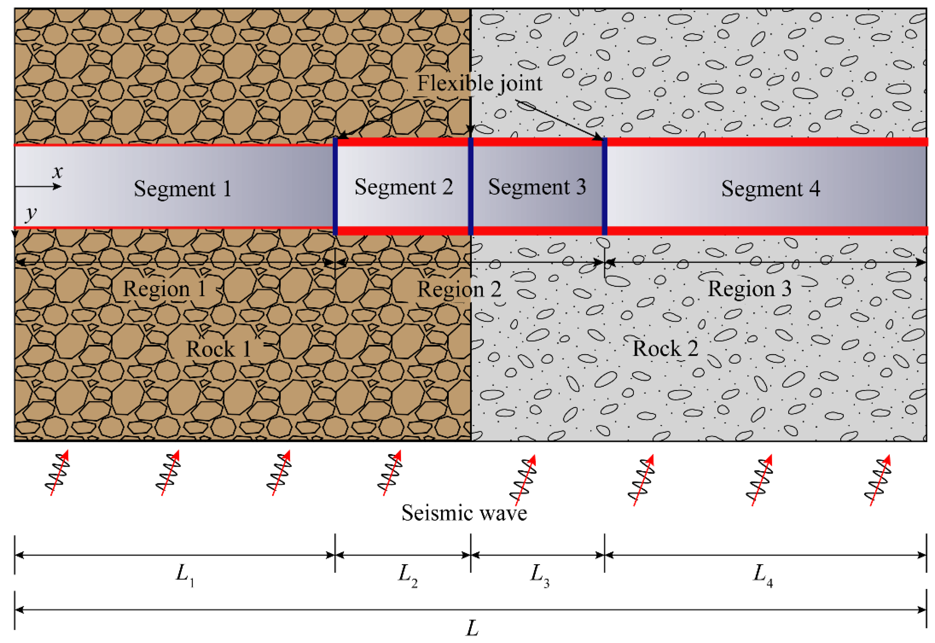
Figure 2.
Analytical model.
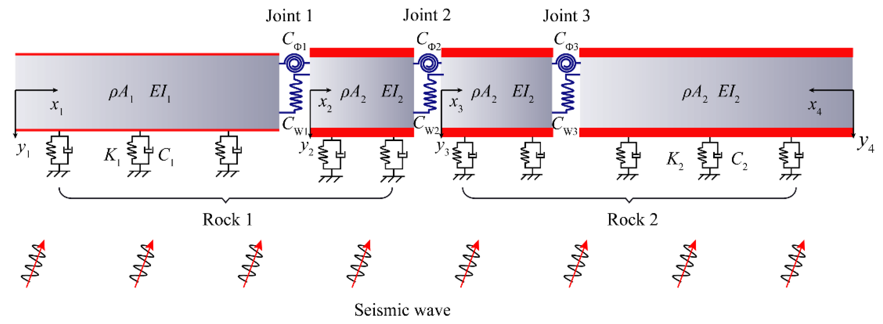
Figure 3.
Input earthquake wave.

Figure 4.
Responses of a tunnel buried in non-homogeneous ground (case 1).
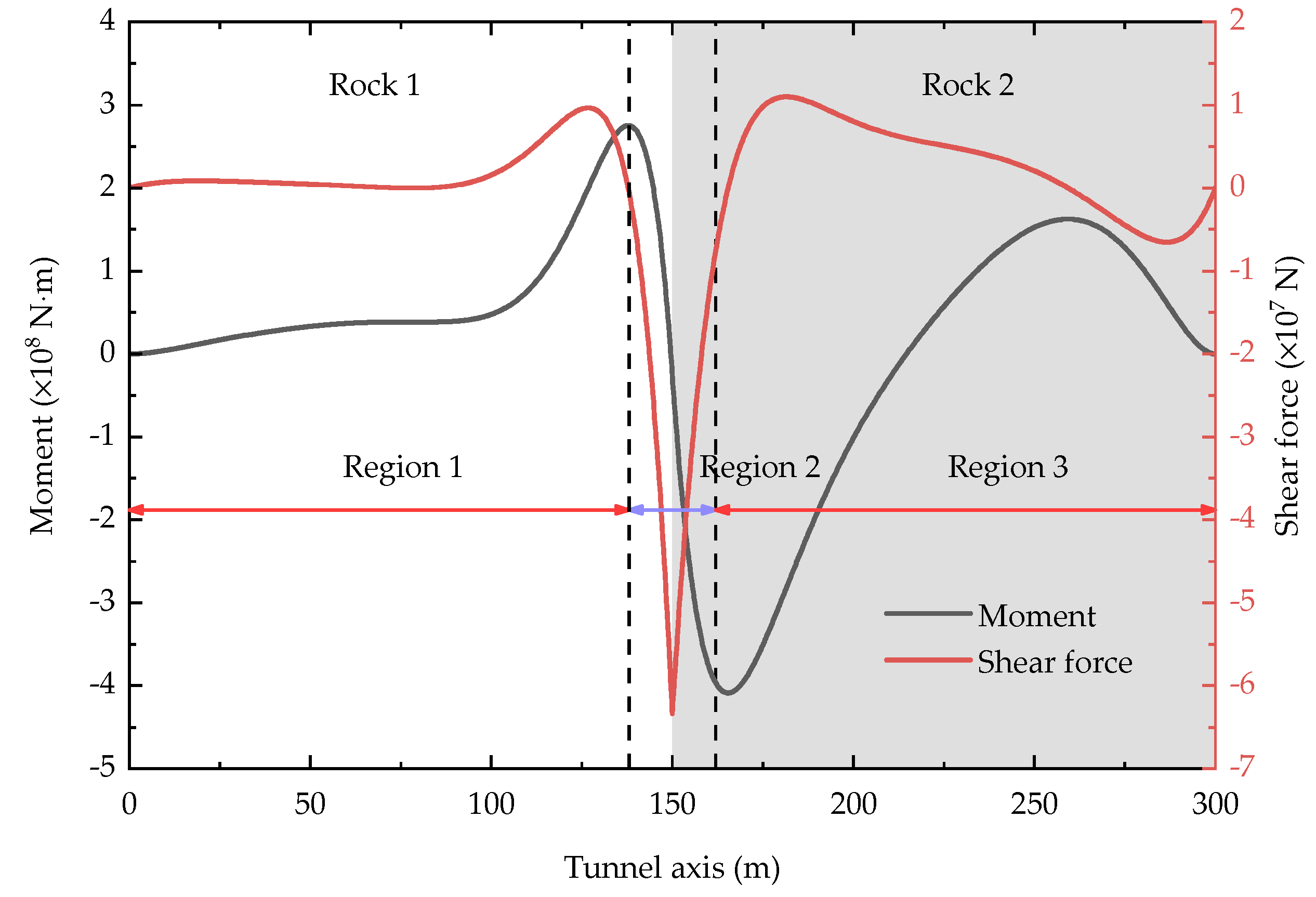
Figure 5.
Influences of the soft-hard stratum junction on normalized internal forces. (a) Normalized bending moment; (b) normalized shear force.
Figure 5.
Influences of the soft-hard stratum junction on normalized internal forces. (a) Normalized bending moment; (b) normalized shear force.
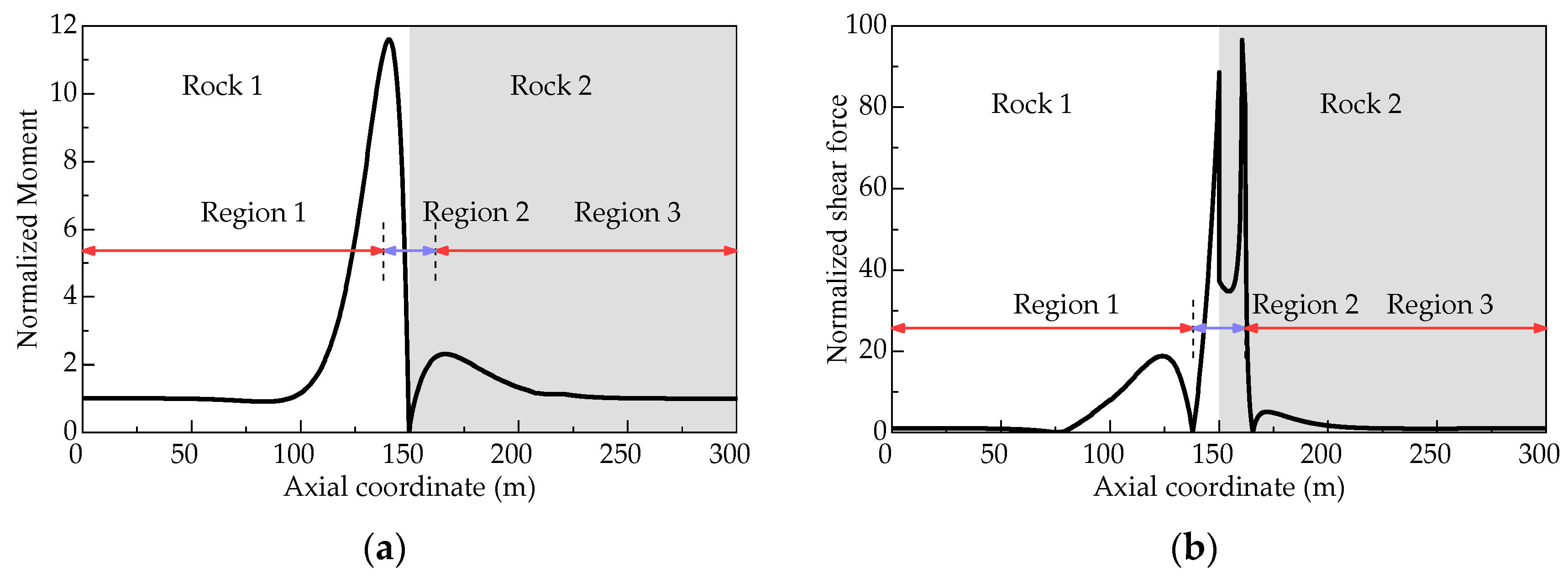
Figure 6.
Displacement along the tunnel axis.
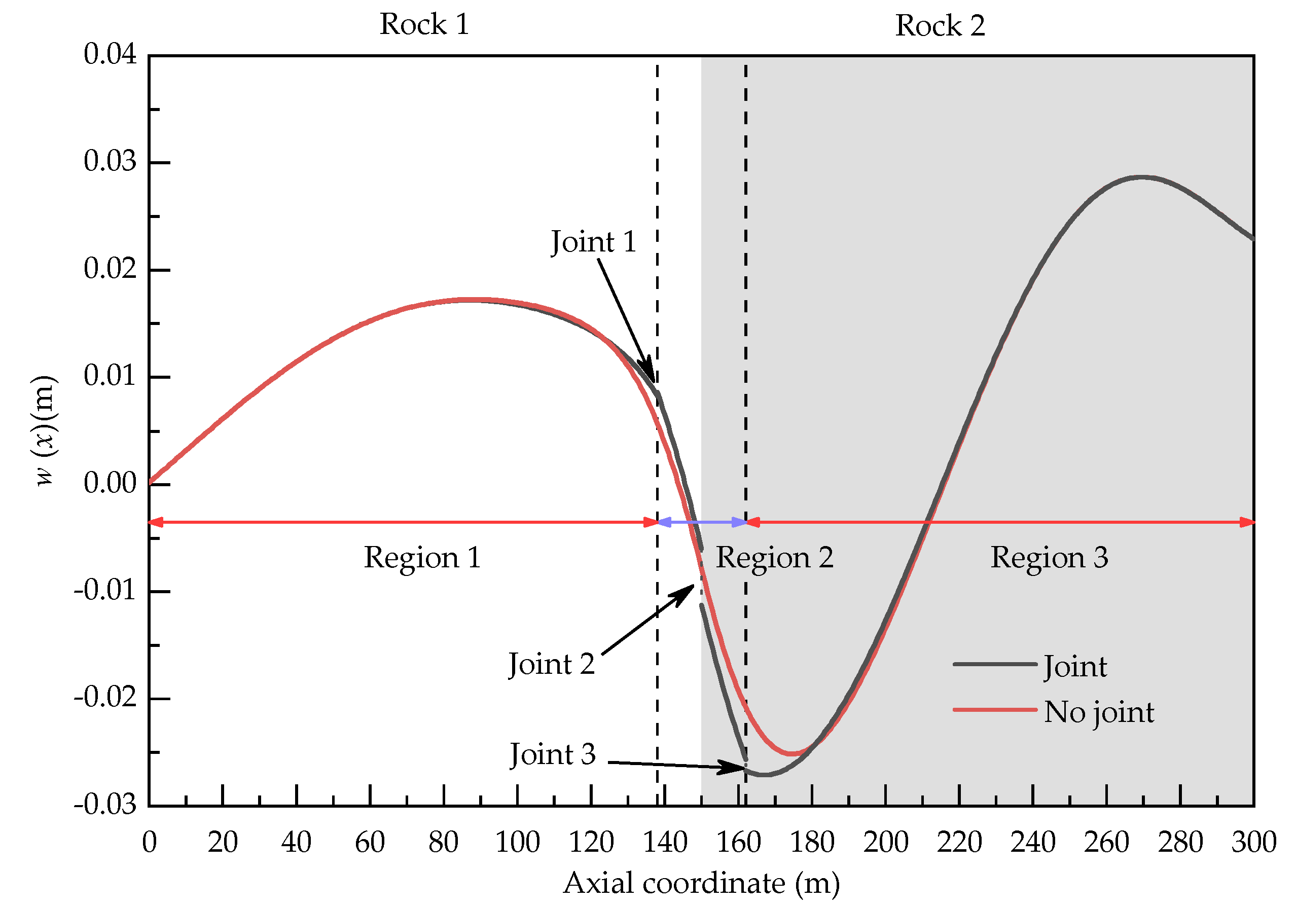
Figure 7.
Influence of the joint on tunnel responses. (a) Bending moment; (b) shear force.
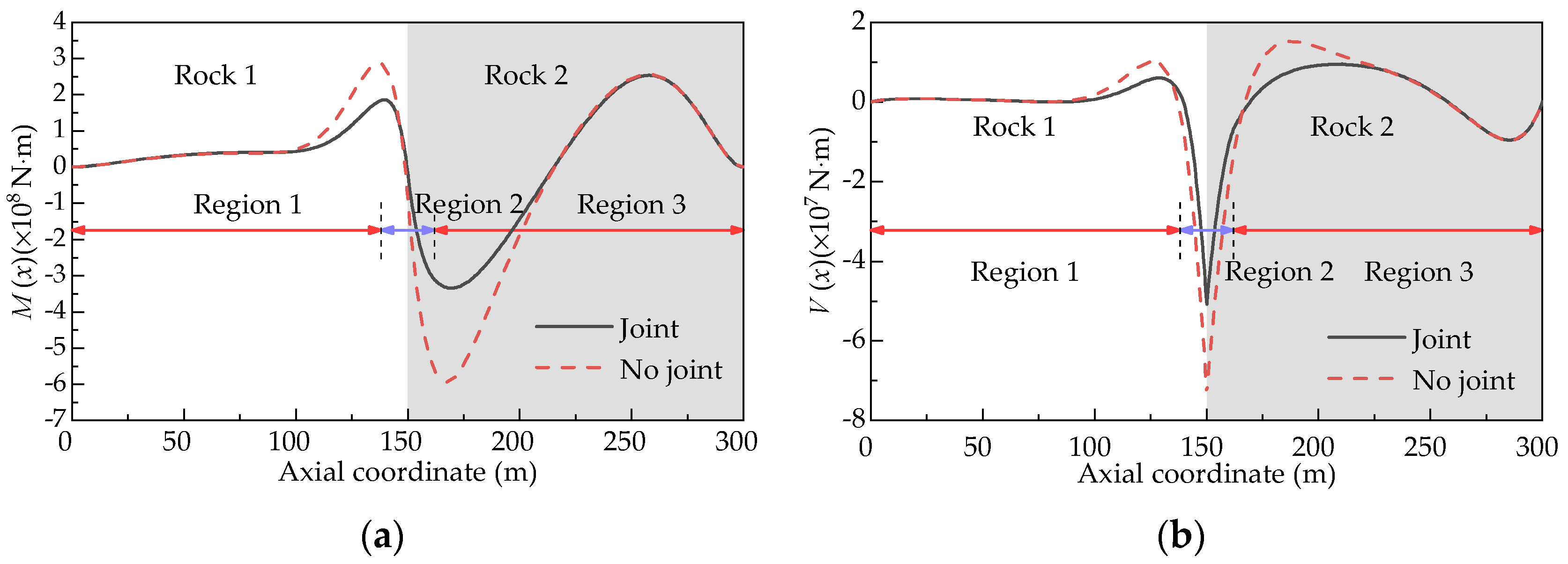
Figure 8.
Effect of the length of the transition zone on internal forces. (a) Bending moment; (b) shear force.
Figure 8.
Effect of the length of the transition zone on internal forces. (a) Bending moment; (b) shear force.

Figure 9.
Model soil interface control.

Figure 10.
Jointed lining segments.
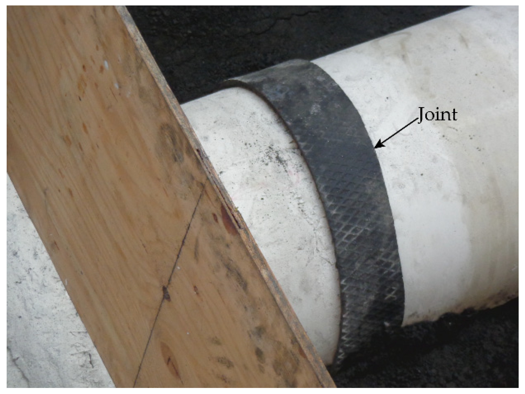
Figure 11.
Instrumentation for the shaking table tests.

Figure 12.
Input earthquake wave. (a) Acceleration time histories; (b) Fourier spectra.
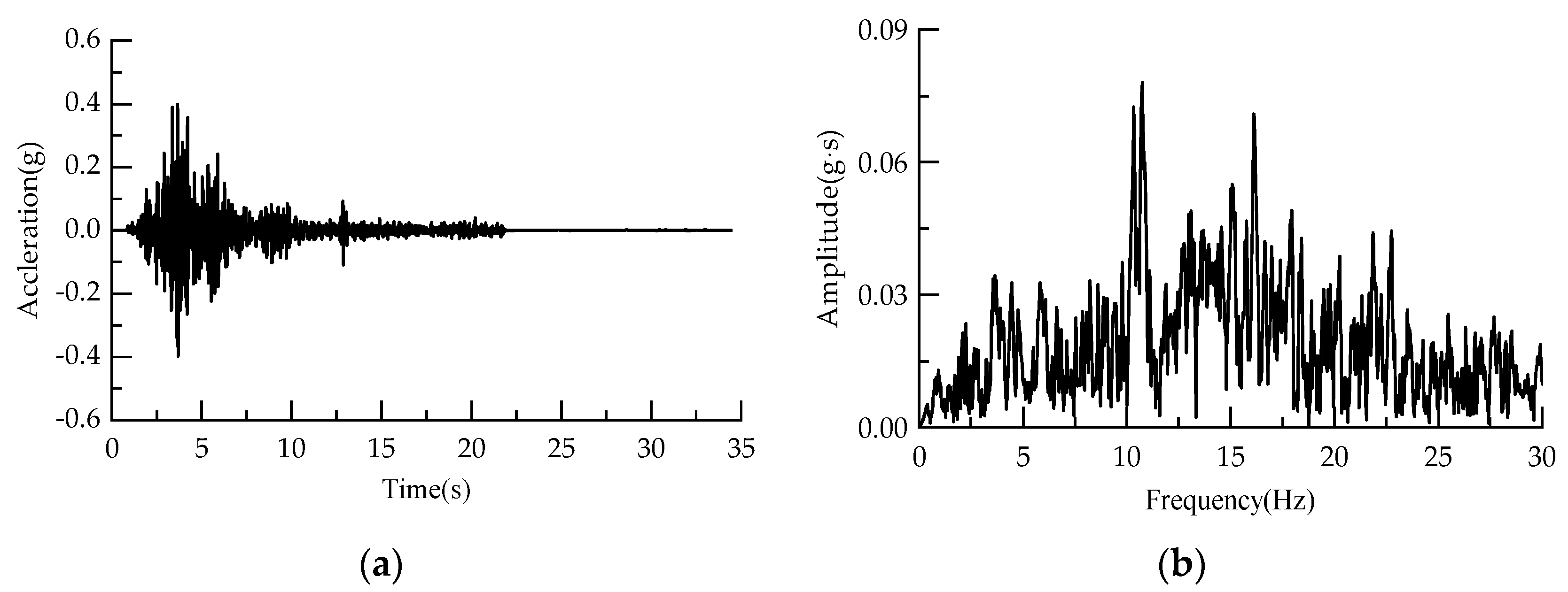
Figure 13.
Comparison of bending moments of lining between the theoretical analysis and the model tests.
Figure 13.
Comparison of bending moments of lining between the theoretical analysis and the model tests.

Figure 14.
Peak strains of measuring points for excitations with different amplitudes. (a) 0.2 g; (b) 0.4 g.
Figure 14.
Peak strains of measuring points for excitations with different amplitudes. (a) 0.2 g; (b) 0.4 g.
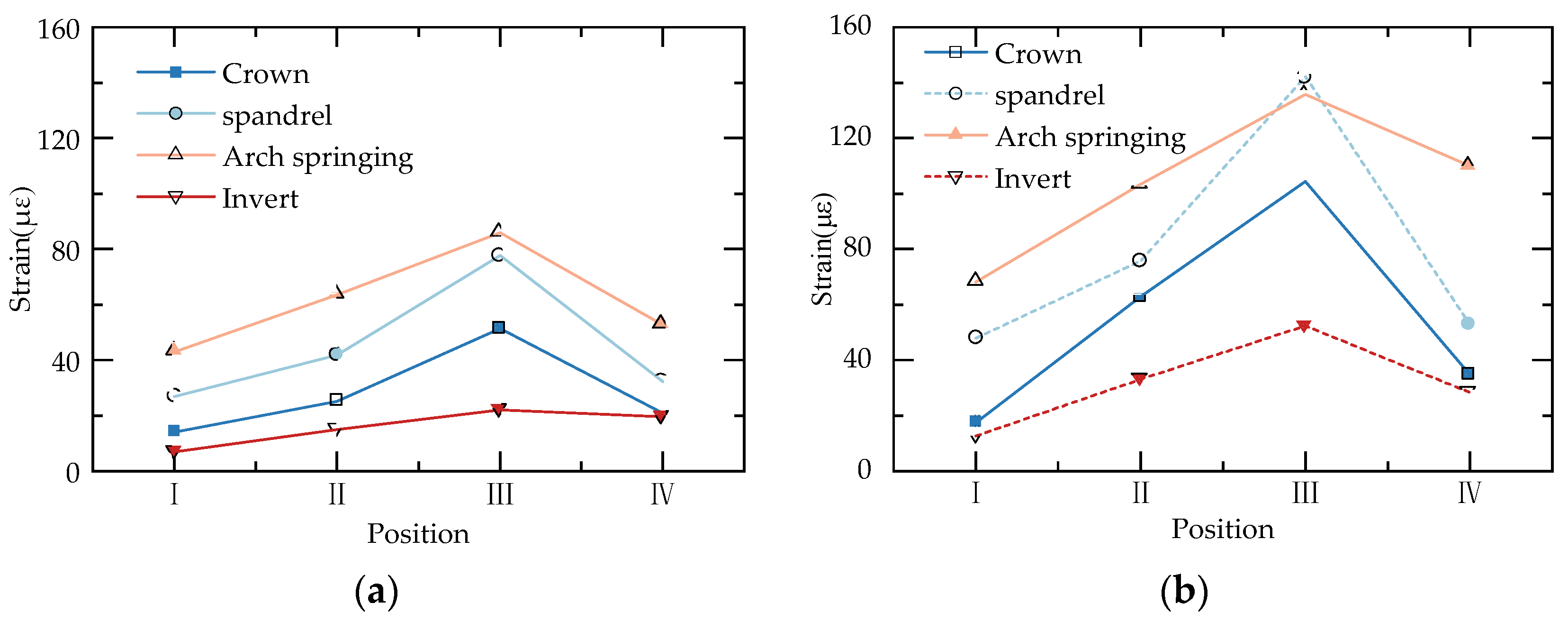
Figure 15.
Acceleration records and Fourier spectra of monitoring positions in the shaking table tests. (a) Acceleration time history and Fourier spectrum of monitoring point A1; (b) acceleration time history and Fourier spectrum of monitoring point A3; (c) acceleration time history and Fourier spectrum of monitoring point A4; (d) acceleration time history and Fourier spectrum of monitoring point A5.


Table 1.
Similarity relation for shaking table tests.
| Physical Quantity | Length | Density | Young’s Modulus | Cohesion | Friction Angle | Strain |
|---|---|---|---|---|---|---|
| Similarity relation | Cl | Cρ | CE | CC = CE | Cφ | Cε |
| Ratio of similarity ratio | 1/30 | 1/1.5 | 1/45 | 1/45 | 1 | 1 |
Table 2.
Parameters of the model.
| Name | Young’s Modulus (GPa) | Density (kg/m3) | Cohesion (kPa) | Friction Angle (°) | Poisson’s Ratio | Compression Strength (MPa) |
|---|---|---|---|---|---|---|
| Rock model | 0.06 | 1467 | 16.5 | 32.3 | - | - |
| Fault model | 0.02 | 1200 | 4.0 | 25 | - | - |
| Lining model | 0.68 | 1600 | - | - | 0.25 | 0.53 |
Publisher’s Note: MDPI stays neutral with regard to jurisdictional claims in published maps and institutional affiliations. |
© 2022 by the authors. Licensee MDPI, Basel, Switzerland. This article is an open access article distributed under the terms and conditions of the Creative Commons Attribution (CC BY) license (https://creativecommons.org/licenses/by/4.0/).
Share and Cite
MDPI and ACS Style
Yan, G.; Zhao, B. Analytical Solution and Shaking Table Test on Tunnels through Soft-Hard Stratum with a Transition Tunnel and Flexible Joints. Appl. Sci. 2022, 12, 3151. https://doi.org/10.3390/app12063151
AMA Style
Yan G, Zhao B. Analytical Solution and Shaking Table Test on Tunnels through Soft-Hard Stratum with a Transition Tunnel and Flexible Joints. Applied Sciences. 2022; 12(6):3151. https://doi.org/10.3390/app12063151
Chicago/Turabian StyleYan, Gaoming, and Boming Zhao. 2022. "Analytical Solution and Shaking Table Test on Tunnels through Soft-Hard Stratum with a Transition Tunnel and Flexible Joints" Applied Sciences 12, no. 6: 3151. https://doi.org/10.3390/app12063151
Note that from the first issue of 2016, this journal uses article numbers instead of page numbers. See further details here.