Featured Application
Convolutional neural networks are used on the channel impulse response data to predict the performance of underwater acoustic communications.
Abstract
Predicting the channel quality for an underwater acoustic communication link is not a straightforward task. Previous approaches have focused on either physical observations of weather or engineered signal features, some of which require substantial processing to obtain. This work applies a convolutional neural network to the channel impulse responses, allowing the network to learn the features that are useful in predicting the channel quality. Results obtained are comparable or better than conventional supervised learning models, depending on the dataset. The universality of the learned features is also demonstrated by strong prediction performance when transferring from a more complex underwater acoustic channel to a simpler one.
1. Introduction
Underwater acoustic (UWA) propagation is a complex probabilistic process dependent on many time-varying factors. For the general communication system, it is often desirable to establish a relationship between channel characteristics and the receiver decoding performance; however, the complex UWA environment often makes this a challenging task. Reliable prediction of the UWA communication performance is an enabling technology for many useful methods and systems, including adaptive networking and adaptive modulation strategies [1,2], for both point-to-point communications and underwater sensor networks; please refer to [3,4] for corresponding system characteristics and challenges.
Previous works have focused largely on utilizing meteorological data [5] or signal statistics as input features [6]. These features are either observed directly through additional sensors, such as the meteorological data, or are engineered features estimated from signal statistics.
The communication performance prediction is often cast as a classification problem by establishing ranges of performance. In the broader field of wireless sensor networks, decision trees and rule sets were introduced in [7] to predict a class of bit error rate (BER) to make routing decisions. Logistic regression was employed in [5] to estimate a range of packet success ratios based on environmental factors. A boosted regression tree was used in [2] to estimate the BER based on channel parameters such as the signal-to-noise ratio (SNR) and the delay spread, in order to apply an adaptive modulation scheme.
In our earlier work [8], taking as inputs the engineered features derived from the full communication waveform, conventional regression methods and classification methods were applied to predict the communication performance. Specifically, for the orthogonal frequency-division multiplexing (OFDM) system, the derived engineered features include the time-domain SNR, the pilot SNR that measures the SNR in the frequency domain in the presence of Doppler effect, and the channel root-mean-square delay spread. Despite providing reasonable prediction performance, deriving those features requires knowledge of the full OFDM waveform and additional receiver processing.
To create a method that can be extended to the scenario where the full waveform is not available or costly to obtain, this work studies the performance prediction based on channel impulse responses (CIRs). Compared to the engineered features, the CIR can be easily obtained with an impulsive source or derived from a known broadband signal; a chirp is often used as part of the preamble in many UWA communications for channel sounding. In addition, the CIR contains more information than the engineered features.
Convolutional neural networks (CNNs) have been heavily used in the field of computer vision and have been a breakthrough technology in the areas of image classification [9] and object detection [10]. Image processing methods have been extended to the domain of audio recognition by featurizing the audio signal into a 2D image through the use of mel-spectrograms and other related representations [11]. More recent work in the area of sound classification has explored the use of CNNs that only operate in one dimension [12].
Our work attempts to start with the CIR, a minimally processed input, and utilizes a CNN to interpret a meaningful performance prediction from that. The ability of the trained CNN as a feature extraction system is also explored by generating features and using them in conventional models. The proposed method can be extended to more challenging UWA channels, such as those with impulsive noise [13], by combining the CIR with impulsive noise for feature extraction.
The rest of this paper is organized as follows. The data used for this work, including pre-processing used for conventional methods is presented in Section 2. The processing methods, both conventional and the proposed CNN method are introduced in Section 3. Results of the conventional methods are presented in Section 4. Results using the proposed CNN method are presented in Section 5. A study of model transferability between different models is covered in Section 6. Conclusions are drawn in Section 7.
2. Datasets
Two datasets are used to evaluate the methods described in this work, one dataset collected in the Keweenaw Waterway in August, 2014, (abbreviated as KWAUG14) [14] and the other dataset from the Surface Processes and Acoustic Communication Experiment performed off the coast of Martha’s Vineyard in 2008 (abbreviated as SPACE08) [15].
- The KWAUG14 experiment lasted about 4.5 days. The water depth was about 10 m. A waveform of 8.8 s in the frequency band kHz was transmitted with a fixed power every 15 min over a link of 312 m. The waveform is modulated by the orthogonal frequency-division multiplexing (OFDM) technique with a quadrature shift keying (QPSK) constellation. Each transmission consists of 20 OFDM blocks.
- The SPACE08 experiment was conducted off the coast of Martha’s Vineyard at the Air-Sea Interaction Tower by Woods Hole Oceanographic Institution from 14 October to 1 November 2008 [15]. The water depth was about 15 m. An OFDM communication waveform within the frequency band kHz was transmitted every two hours. The experiment consisted of several different receiver arrays, but to commonize the datasets, in this work only the data collected from a single receiver array (S3, located 200 m from the source) and modulated by the QPSK constellation are used.
The KWAUG14 experiment took place in fresh water with mostly good weather conditions, while The SPACE08 experiment took place in the sea environment over a wider variety of weather conditions. Additional measurements of turbulence, turbidity, and temperature are not included in this study. It is expected that additional variation of these parameters would create a more diverse set of multipath effects and this warrants further study.
While only a single transmission distance from each dataset is included in this work, our previous work [8] considered different receiver arrays from the SPACE08 experiment and showed that the conventional methods worked well on the shorter and longer distance channels, at 60 m and 1 km respectively. The influence of temperature and ice cover isn’t considered in this work, but a study of channel condition variation [16] shows that an observable difference in CIRs and SNR is present with ice cover. It is expected that these changes (different transmission range, temperature, and ice cover) could be learned by the methods proposed in Section 5.
Feature Extraction
To shed insights into the CIRs from two experiments, two features are extracted from the CIRs. The CIR shows a representation of the multi-path channel between the source and the receiver as a convolutional system, with copies of the transmitted signal arriving at the receiver with different delays (sometimes referred to as arrivals). In order to use traditional supervised learning methods with the relatively long CIR, it is necessary create low dimensional representations, which are known as features. The first feature generated is an estimate of the SNR, in which the CIR before the first arrival is used to estimate the noise variance and everything over three times the noise standard deviation is considered to be an arrival. The delay spread is also calculated, which measures the time difference between the first arrival and the last arrival in milliseconds. An example of this processing can be seen in Figure 1, which shows data from an arbitrarily selected CIR from the KWAUG14 dataset. The two significant arrivals are identified by a marker; in this example, SNR is calculated to be 14.1 dB and the delay spread is 1.17 milliseconds.
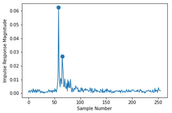
Figure 1.
An example of feature extraction from the KWAUG14 channel impulse response. Significant arrivals have a marker.
To better understand the distribution of these features for both datasets, crossplots of the extracted features and the BERs are generated and shown in Figure 2 and Figure 3. Due to the high density of points, density contours are shown on the lower off-diagonal crossplots to aid interpretation. There are some obvious trends, such as a weak inverse relationship between the SNR and the BER and different regimes of delay spreads that don’t correlate well to BER.
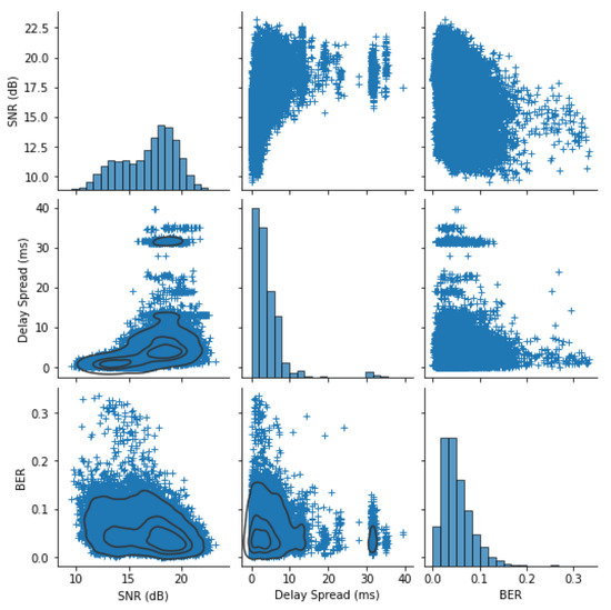
Figure 2.
KWAUG14: extracted feature distributions with kernel density estimate contours on lower left off-diagonal plots.
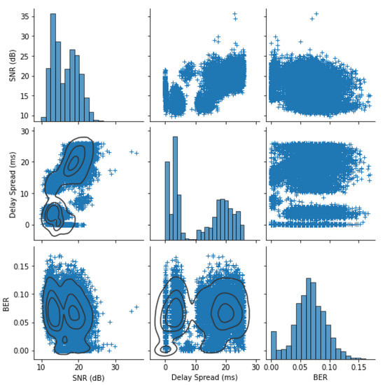
Figure 3.
SPACE08: extracted feature distributions with kernel density estimate contours on lower left off-diagonal plots.
For KWAUG14, due to the relatively static channel condition, a fairly consistent delay spread and low BERs can be observed in Figure 2. The trend between the SNR and the BER is not strong, but shows the slight negative trend one would expect.
For SPACE08, one can observe from Figure 3 that the CIR is much more complex and includes arrivals with a longer delay spread than KWAUG14. In addition, the CIRs vary substantially between measurements. The average BER is higher, but the weak negative trend between SNR and BER is still visible.
3. Methods
3.1. Convolutional Neural Network Architecture
The neural network design utilized in this work is based on the basic architecture used for some of the first successful convolutional neural networks proposed by LeCun [17]. Instead of using two-dimensional convolutional layers, as one would use for an image, this network uses one-dimensional convolutional layers. The input layer takes in the real and imaginary parts of the CIR as separate channels. Early investigations found that a real/imaginary representation performs better than a magnitude/phase representation, probably due to the lack of a jump introduced by the phase wrap [18].
The CNN is constructed using the Tensorflow library [19]. The CNN architecture is depicted in Figure 4. Each convolutional layer consists of 40 learned filters and uses a rectified linear unit [20] as the activation function. This is followed by a dropout layer to help prevent overfitting [21] and a maximum pooling layer. The pooling reduces the dimensionality, improves invariance to translation, decreases the processing time, and changes the scale of features being learned by the next convolutional layer. After four layers of this, the output of the pooling layer is flattened and attached to a fully-connected 100-element layer. To facilitate the use of this network for featurizing, a second eight-element layer is included before the regression output layer.
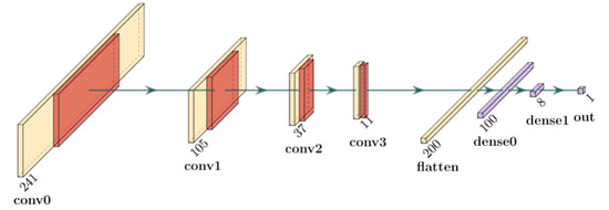
Figure 4.
Diagram of the proposed CNN architecture.
3.2. Conventional Regression Methods
The conventional regression models are included for the thoroughness of this work. The list of models considered is not exhaustive, but it includes a variety of methods. Some are selected for their simplicity and others are chosen for their capability. For example, the dummy method will always output the same value and provides a lower bound that any useful method should exceed.
The conventional regression methods used in this paper include:
- Linear Regression: A common numerical approach where each feature contributes linearly to the regressed output [22];
- Two-Layer Neural Network: The two-layer fully connected neural network has a capability of approximating any function [23];
- K-Nearest Neighbors: K-Nearest Neighbors (KNN) uses the data as the model and uses the nearest K points in the feature space to determine the regressed value [24];
- Dummy: This is a simple method that ignores input data and creates outputs based only on the training data; the version used for this work outputs the median value of the BER observed in the training data [25];
- Decision Tree: Decision trees are well studied graph-based methods where each node splits based on feature values. The specific decision tree utilized in this work is the Classification and Regression Tree (CART) algorithm [26] implemented in Scikit-learn [25].
3.3. Conventional Regression Methods with CNN-Derived Features
The neural network can be used as a featurizer by removing the final output regression layer and using the previous fully connected layer as the outputs. Because the network has already been trained to perform the task of predicting the BER, information related to the task is represented by the outputs of this layer. This can be thought of as a form of data compression. Similar work has been performed using autoencoders to generate compressed representations of the CIRs in massive multi-input multi-output systems [18].
3.4. Evaluation Metrics
Two different metrics are used to evaluate the success of each method, mean absolute error (MAE) and Pearson correlation coefficient. Mean absolute error is a common method for evaluating a regression method and is in units that are directly understandable [27]. Pearson correlation coefficient provides additional insight into regression performance by giving an indication of the linearity of the regression [28]. For each method studied, five fold cross validation is used with randomly selected groupings. In each table of reported results, the mean of the five folds is reported alongside the standard deviation, which is in parentheses. A one-sided, two sample t-test is used to determine if any other methods are statistically similar to the method with the lowest error. The method with the lowest error is bolded and any other method that is not significantly different (p > 0.05) is also bolded.
4. Results of Conventional Regression Methods with Traditional Features
In our previous work [8], traditional engineered features were derived from the full OFDM waveform and were used with conventional regression methods to predict the communication performance. For the purposes of this paper, traditional features refers to signal statistics derived from the OFDM waveform, such as SNR and delay spread. For prediction performance comparison with CIR-based methods, Table 1 lists the prediction performance based on the features derived from the full OFDM waveform, including the time-domain SNR and the delay spread. While performance for most methods is quite good, the decision tree performs best for KWAUG14 and the linear regression works best for SPACE08.

Table 1.
Conventional regression results using traditionally available features.
5. Results of the CIR-Based Methods
This section will present the prediction performance of several CIR-based methods.
5.1. Conventional Regression Method Results with CIR-Derived Features
To provide a bridge from the previous work using traditionally available features [8], engineered features derived only from CIRs are considered using the conventional regression methods. The results are shown in Table 2. Compared to Table 1, it can be seen that traditionally available features perform better with these methods, as the features derived from the full OFDM waveform capture additional information not available in features derived solely from the CIR.
Table 2.
Conventional regression results using CIR-derived features.
5.2. CNN Results
The proposed CNN architecture in Figure 4 is able to directly work on the CIR, which has benefits of reducing the operator influence. The results of the CNN method are shown in Table 3. Compared to the results in Table 1, the CNN results are close to the best performance using traditional features for the KWAUG14 dataset and superior for the more complex SPACE08 dataset. When both datasets are combined into one dataset, the model still performs well, close to or even better than independent models.
Table 3.
Convolutional neural network regression results.
5.3. Conventional Regression Methods with CNN Features
For certain applications, such as model interpretability, it may be desirable to utilize a traditional model. By using the penultimate layer of the CNN as the output, features are extracted and fed into the previously used conventional models. The results of this method can be seen in Table 4. Results are nearly identical to the CNN results.
Table 4.
Conventional regression results using CNN-derived features.
6. Transfer Learning between Datasets
To understand the universality of these models, it is informative to attempt transferring a learned model between the datasets. As discussed above, although both datasets could be described as from a “shallow water” environment, they vary quite substantially in terms of physical environment and the data observed reflects that. This makes them a useful pair of datasets for evaluating the transferability of these models.
6.1. Conventional Regression Models
For completeness and to provide a reference, the conventional models are transferred first. They are trained on the training split of one dataset’s and evaluated on the test split of the other dataset. The results are shown in Table 5. Interestingly, they perform about as well as the original models (cf. Table 2).
Table 5.
Conventional regression results with transfer learning using CIR-derived features.
6.2. CNN-Based Models
Transfer of the CNN-based model is explored as well. The results can be seen in Table 6. The model trained on the SPACE08 dataset perform decently well on the KWAUG14 dataset, although that does not work as well in reverse. This is a reasonable result, as the KWAUG14 dataset is fairly homogeneous in terms of environmental conditions while the SPACE08 data took place over several days with a wide variety of weather conditions.
Table 6.
Convolutional neural network transfer learning regression results.
7. Conclusions
In this work, we explored the use of 1D CNNs for performance prediction based on the CIR in UWA communications. We compared the results with those of conventional machine learning methods using traditionally available channel features as well as the features derived only from the CIRs. A brief investigation of using the trained CNN as a featurizer was also performed. This featurizer method opens up opportunities for easier implementation, as the convolutional layers could be implemented as FIR filters and less computation could be required within an adaptive modem or other application of this method. It was demonstrated that on a varied dataset such as SPACE08, the CNN-based methods can outperform conventional ones and their performances are comparable when using on a homogeneous dataset. The results in this work revealed that the CNN is a promising technique to extract useful information from UWA channels.
Author Contributions
Conceptualization, E.L. and Z.W.; methodology, E.L. and Z.W.; software, E.L.; validation, E.L.; formal analysis, E.L. and Z.W.; investigation, Z.W.; resources, Z.W.; data curation, E.L. and Z.W.; writing—original draft preparation, E.L.; writing—review and editing, E.L. and Z.W.; visualization, E.L.; supervision, Z.W.; project administration, Z.W.; funding acquisition, Z.W. All authors have read and agreed to the published version of the manuscript.
Funding
This work was supported by the NSF grant ECCS-1651135 (CAREER).
Institutional Review Board Statement
Not applicable.
Informed Consent Statement
Not applicable.
Data Availability Statement
The data presented in this study are available on request from the corresponding author.
Conflicts of Interest
The authors declare no conflict of interest.
Abbreviations
The following abbreviations are used in this manuscript:
| CIR | Channel Impulse Response |
| CNN | Convolutional Neural Network |
| KNN | K-Nearest Neighbors |
| KWAUG14 | Keweenaw Waterway August 2014 experiment |
| MAE | Mean Absolute Error |
| QPSK | Quadrature Phase Shift Keying |
| SNR | Signal-to-Noise Ratio |
| SPACE08 | Surface Processes and Acoustic Communication Experiment 2008 |
| UWA | Underwater Acoustic |
References
- Wang, C.; Wang, Z.; Sun, W.; Fuhrmann, D.R. Reinforcement learning-based adaptive transmission in time-varying underwater acoustic channels. IEEE Access 2017, 6, 2541–2558. [Google Scholar]
- Pelekanakis, K.; Cazzanti, L. On adaptive modulation for low SNR underwater acoustic communications. In Proceedings of the OCEANS 2018 MTS/IEEE Charleston, Charleston, SC, USA, 22–25 October 2018. [Google Scholar]
- Heidemann, J.; Stojanovic, M.; Zorzi, M. Underwater sensor networks: Applications, advances and challenges. Philos. Trans. R. Soc. A Math. Phys. Eng. Sci. 2012, 370, 158–175. [Google Scholar]
- Alfouzan, F.A. Energy-efficient collision avoidance MAC protocols for underwater sensor networks: Survey and challenges. J. Mar. Sci. Eng. 2021, 9, 741. [Google Scholar]
- Kalaiarasu, V.; Vishnu, H.; Mahmood, A.; Chitre, M. Predicting underwater acoustic network variability using machine learning techniques. In Proceedings of the CEANS 2017-Anchorage, Anchorage, AK, USA, 18–21 September 2017. [Google Scholar]
- Pelekanakis, K.; Cazzanti, L.; Zappa, G.; Alves, J. Decision tree-based adaptive modulation for underwater acoustic communications. In Proceedings of the 2016 IEEE Third UNDERWATER communications and networking Conference (UComms), Lerici, Italy, 30 August–1 September 2016; pp. 1–5. [Google Scholar]
- Wang, Y.; Martonosi, M.; Peh, L.S. Predicting link quality using supervised learning in wireless sensor networks. ACM Sigmobile Mob. Comput. Commun. Rev. 2007, 11, 71–83. [Google Scholar]
- Lucas, E.; Wang, Z. Supervised Learning for Performance Prediction in Underwater Acoustic Communications. In Proceedings of the Global Oceans 2020: Singapore–US Gulf Coast, Biloxi, MS, USA, 5–30 October 2020; pp. 1–6. [Google Scholar]
- Simonyan, K.; Zisserman, A. Very deep convolutional networks for large-scale image recognition. arXiv 2014, arXiv:1409.1556. [Google Scholar]
- Bochkovskiy, A.; Wang, C.Y.; Liao, H.Y.M. Yolov4: Optimal speed and accuracy of object detection. arXiv 2020, arXiv:2004.10934. [Google Scholar]
- Piczak, K.J. Environmental sound classification with convolutional neural networks. In Proceedings of the 2015 IEEE 25th International Workshop on Machine Learning for Signal Processing (MLSP), Gold Coast, Australia, 20–23 September 2015; pp. 1–6. [Google Scholar]
- Abdoli, S.; Cardinal, P.; Koerich, A.L. End-to-end environmental sound classification using a 1D convolutional neural network. Expert Syst. Appl. 2019, 136, 252–263. [Google Scholar]
- Wang, J.; Li, J.; Yan, S.; Shi, W.; Yang, X.; Guo, Y.; Gulliver, T.A. A novel underwater acoustic signal denoising algorithm for Gaussian/non-Gaussian impulsive noise. IEEE Trans. Veh. Technol. 2020, 70, 429–445. [Google Scholar]
- Sun, W.; Wang, Z. Modeling and prediction of large-scale temporal variation in underwater acoustic channels. In Proceedings of the OCEANS 201-6 Shanghai, Shanghai, China, 10–13 April 2016. [Google Scholar]
- Zhou, S.; Wang, Z. OFDM for Underwater ACOUSTIC Communications; John Wiley & Sons: Hoboken, NJ, USA, 2014. [Google Scholar]
- Sun, W.; Wang, C.; Wang, Z.; Song, M. Experimental comparison between under-ice and open-water acoustic channels. In Proceedings of the 10th International Conference on Underwater Networks & Systems, Arlington, VA, USA, 22–24 October 2015; pp. 1–2. [Google Scholar]
- LeCun, Y. Generalization and network design strategies. Connect. Perspect. 1989, 19, 143–155. [Google Scholar]
- Yang, Q.; Mashhadi, M.B.; Gündüz, D. Deep convolutional compression for massive MIMO CSI feedback. In Proceedings of the 2019 IEEE 29th International Workshop on Machine Learning for Signal Processing (MLSP), Pittsburgh, PA, USA, 13–16 October 2019; pp. 1–6. [Google Scholar]
- Abadi, M.; Agarwal, A.; Barham, P.; Brevdo, E.; Chen, Z.; Citro, C.; Corrado, G.S.; Davis, A.; Dean, J.; Devin, M.; et al. TensorFlow: Large-Scale Machine Learning on Heterogeneous Systems. 2015. Available online: www.tensorflow.org (accessed on 24 December 2021).
- Arora, R.; Basu, A.; Mianjy, P.; Mukherjee, A. Understanding deep neural networks with rectified linear units. arXiv 2016, arXiv:1611.01491. [Google Scholar]
- Baldi, P.; Sadowski, P.J. Understanding dropout. Adv. Neural Inf. Process. Syst. 2013, 26, 2814–2822. [Google Scholar]
- Bishop, C.M. Pattern Recognition and Machine Learning; Springer: Berlin/Heidelberg, Germany, 2006. [Google Scholar]
- Goodfellow, I.; Bengio, Y.; Courville, A.; Bengio, Y. Deep Learning; MIT Press: Cambridge, UK, 2016; Volume 1. [Google Scholar]
- Friedman, J.; Hastie, T.; Tibshirani, R. The Elements of Statistical Learning; Springer: New York, NY, USA, 2001; Volume 1. [Google Scholar]
- Pedregosa, F.; Varoquaux, G.; Gramfort, A.; Michel, V.; Thirion, B.; Grisel, O.; Blondel, M.; Prettenhofer, P.; Weiss, R.; Dubourg, V.; et al. Scikit-Learn: Machine Learning in Python. J. Mach. Learn. Res. 2011, 12, 2825–2830. [Google Scholar]
- Breiman, L.; Friedman, J.; Stone, C.J.; Olshen, R.A. Classification and Regression Trees; CRC Press: Boca Raton, FL, USA, 1984. [Google Scholar]
- Willmott, C.J.; Matsuura, K. Advantages of the mean absolute error (MAE) over the root mean square error (RMSE) in assessing average model performance. Clim. Res. 2005, 30, 79–82. [Google Scholar]
- Schober, P.; Boer, C.; Schwarte, L.A. Correlation coefficients: Appropriate use and interpretation. Anesth. Analg. 2018, 126, 1763–1768. [Google Scholar]
- Refaeilzadeh, P.; Tang, L.; Liu, H. Cross-validation. Encycl. Database Syst. 2009, 5, 532–538. [Google Scholar]
Publisher’s Note: MDPI stays neutral with regard to jurisdictional claims in published maps and institutional affiliations. |
© 2022 by the authors. Licensee MDPI, Basel, Switzerland. This article is an open access article distributed under the terms and conditions of the Creative Commons Attribution (CC BY) license (https://creativecommons.org/licenses/by/4.0/).