APF-IRRT*: An Improved Informed Rapidly-Exploring Random Trees-Star Algorithm by Introducing Artificial Potential Field Method for Mobile Robot Path Planning

Abstract

An Informed RRT* (IRRT*) algorithm is one of the optimized versions of a Rapidly-exploring Random Trees (RRT) algorithm which finds near-optimal solutions faster than RRT and RRT* algorithms by restricting the search area to an ellipsoidal subset of the state space. However, IRRT* algorithm has the disadvantage of randomness of sampling and a non-real time process, which has a negative impact on the convergence rate and search efficiency in path planning applications. In this paper, we report a hybrid algorithm by combining the Artificial Potential Field Method (APF) with an IRRT* algorithm for mobile robot path planning. By introducing the virtual force field of APF into the search tree expansion stage of the IRRT* algorithm, the guidance of the algorithm increases, which greatly improves the convergence rate and search efficiency of the IRRT* algorithm. The proposed algorithm was validated in simulations and proven to be superior to some other RRT-based algorithms in search time and path length. It also was performed in a real robotic platform, which shows that the proposed algorithm can be well executed in real scenarios.

1. Introduction

The purpose of mobile robot path planning is to find a feasible and collision-free optimal path from a start point to a target point in an obstacle working environment according to certain evaluation criteria, such as the shortest path length, the minimum energy consumption or the shortest walking time [1,2,3]. As one of the core technologies in mobile robot navigation, path planning ensures that mobile robots can accomplish tasks efficiently, safely and independently, and it has been widely used in motion planning problems, such as in manipulation robots [4], mobile robots [5,6] and unmanned aerial vehicles [7,8]. According to the robot’s knowledge about the environment, path planning is divided into two types [9]: local path planning and global path planning. In local path planning, the robots sense the current local environment (i.e., the location and geometry of the obstacles) and construct an estimated map of the environment in real time during the whole search process to find a feasible obstacle-free path from a start point to a target point. However, this category of path planning can easily conclude with a local optimal solution or even a non-reachable target due to a lack of prior information about the environment. Common local path planning algorithms are the Artificial Immune algorithm [10], A-star algorithm [11], Fuzzy algorithm [12] and APF algorithm [13], etc. In global path planning, owing to knowledge of prior information about the search space, the robots can acquire a global optimal path using optimization algorithms directly. Common global path planning algorithms are the Bee Colony algorithm [14], Genetic algorithm [15] and RRT algorithm [16], etc. Due to the disadvantage of their non-real time process, these algorithms are ineffective if the environment changes, such as an unknown obstacle appearing. Up to now, how to overcome their respective shortcomings and how to realize advantage complementation of different single algorithms remains a technical challenge.

The RRT algorithm, which is considered as one of the most popular global path planning algorithms, is an efficient incremental sampling-based method to find the global solution proposed by S. M. LaValle of Iowa State University in 1998 [16]. The main idea of the RRT algorithm is to construct a search tree rooted at the starting point and to grow the tree by random samples from the search space. The RRT algorithm is simple and can find a solution in any complex environment, and has been widely used in path planning for mobile robots. However, due to the random sampled process, the RRT algorithm usually provides non-optimal solutions. To combat the disadvantages of RRT algorithm, an optimized RRT inversion called RRT star (RRT*) was proposed [17] in 2010. Different from RRT, the RRT* algorithm does not stop sampling after the first solution is found. It continues iteration to optimize the current solution until a near-optimal solution is found. The increased sampling and iteration process also leads to inefficiency of the algorithm.

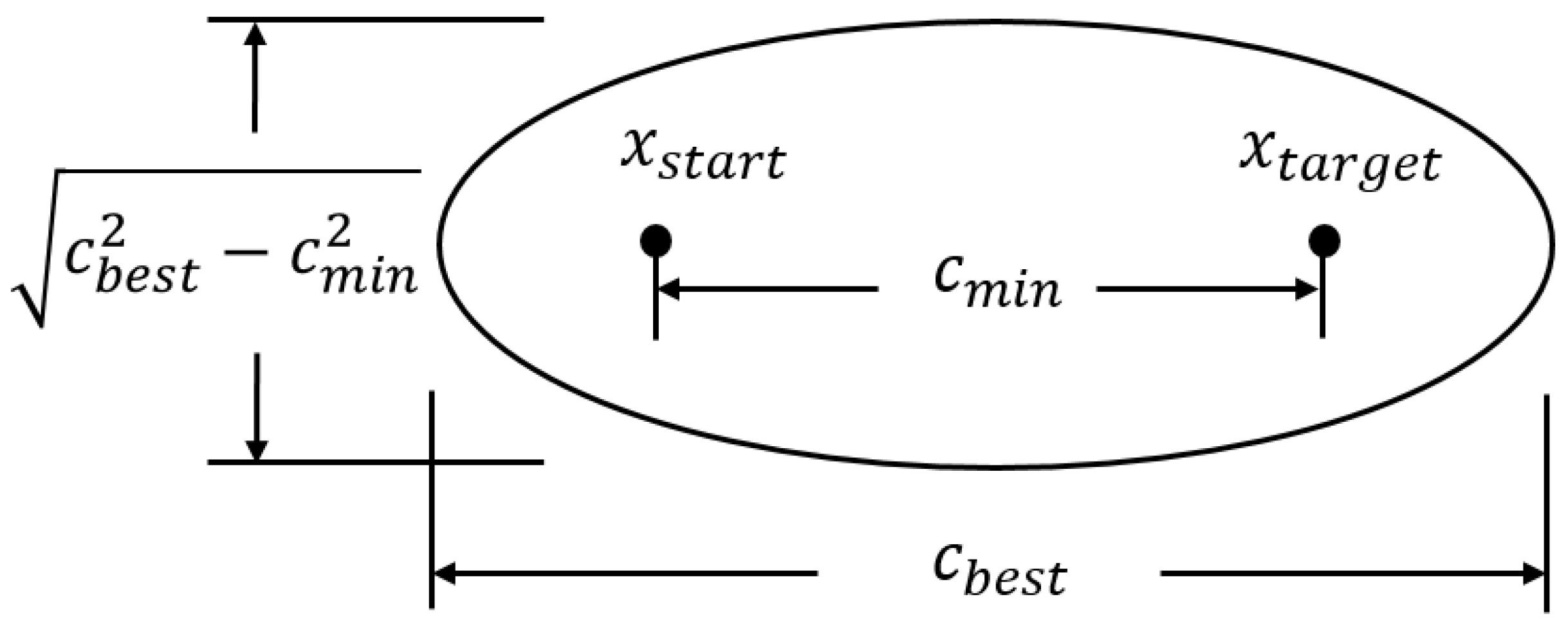
In 2014, Gammell from the University of Toronto further optimized the RRT* algorithm, which is called IRRT* algorithm, by restricting the search area to an ellipsoidal subset of the state space [18,19]. This method expedited the optimization process and improved the rate of convergence while retaining the same probabilistic completeness and asymptotic optimality as the RRT* algorithm. However, it still has the disadvantage of the RRT-based algorithm, in which it is difficult to avoid unnecessary extension and find the optimal solution due to the randomness of sampling and non-real time process.

Due to the disadvantages mentioned above, many algorithms were proposed to improve the quality of RRT-based algorithms. Kuffner proposed the RRT-Connect algorithm in which two search trees were constructed in the start state and target state, respectively, and grew toward each other [20]. This method greatly reduced the search time and improved the efficiency rate. However, due to the random sampling process, the RRT-Connect method still did not optimize their search tree. Wu et al. proposed Fast-RRT which can obtain a new near-optimal path 20 times faster than the RRT* algorithm [21]. To obtain an optimal path, the authors proposed a scheme in which an Improved RRT algorithm is used to quickly search a viable path and a Fast-Optimal algorithm is used to merge it with current best paths.

Recently, another kind of important method, which combines two different single algorithms, was proposed to improve the search efficiency. Brunner introduced A* algorithm into RRT* algorithm to guide the sampling procedure, which greatly accelerates the convergence rate [22]. However, it is inefficient for A* to find an initial solution in a large-scale scenario. Wang et al. applies a reinforcement learning algorithm to an RRT algorithm to direct the growth of search trees [23]. The algorithm developed the exploration ability of each search tree and improved the search efficiency, but the learning-based methods may not perform well in a new environment. In addition, some other hybrid algorithms were proposed to improve the quality of RRT-based path planning algorithms. Jeong et al. proposed the Q-RRT* algorithm which optimized the process of selecting the parent node and connection by using the triangle inequality [24]. The Q-RRT* algorithm obtained a better initial solution and convergence rate than RRT* algorithm. Wang et al. combined a bio-inspired algorithm and RRT algorithm to improve the search speed of finding the initial solution by modifying the sampling process [25]. Their algorithm greatly promoted the convergence rate and saved on memory usage. However, this method led to nonuniform sample distributions. Mashayekhi introduced a hybrid RRT method by combining the RRT-Connect algorithm and IRRT* algorithm [26]. Their algorithm combined the advantages of the two algorithms, which can find initial solutions as quickly as the RRT-Connect algorithm and return the near-optimal solutions as fast as IRRT* method. A. Qurishi et al. proposed P-RRT* algorithm by introducing the APF method into an RRT* algorithm to guide the exploration direction, which accelerated the convergence speed faster than the RRT* algorithm [27]. However, these algorithms only considered the presence of static obstacles and can be only used in global path planning. Up to now, there are only a few reports on path planning algorithms that can be used in complex static and dynamic environments. In 2015, Orozco-Rosas et al. proposed a pseudo-bacterial potential field (PBPF) method [28] by introducing the pseudo-bacterial genetic (PBG) algorithm into the traditional APF method to optimize the gain parameters based on evolutionary computation. Compared with the traditional APF method, the PBPF algorithm provides a simple and powerful way to automatically obtain an optimal value of attractive and repulsive potential gains. Another advantage of the PBPF method is that it is suitable to work in both static and dynamic environments, and it does not need to consider the global map information. Recently, Orozco-Rosas et al. improved their method by combining the APF method with membrane computing with the genetic algorithm [29]. These new algorithms greatly improved the research efficiency by shortening the path length and execution time.

In this paper, we propose a new hybrid APF-IRRT* algorithm by combining the APF algorithm and the IRRT* algorithm. The idea of the virtual force field of APF is introduced into the IRRT* algorithm to guide the random tree to grow towards the goal point, which does not need to model the global environment and avoids random sampling all over the state space. The contributions of the proposed algorithm are: (1) It greatly improves the search efficiency, and reduces the search time by more than 35% and 24% compared with the IRRT* and P-RRT* algorithms, respectively. (2) The APF method increases the guidance for the algorithm, which greatly reduces extended nodes and further shortens the path length and the search time. In addition, the modification of the growth direction of the random tree ensures the optimality of the solution of the algorithm. (3) Compared with most other RRT-based algorithms that can only be applied in static scenarios, the proposed hybrid algorithm includes the advantage of the APF method and can be applied both in static and dynamic environments. The combination of these complementary algorithms also provides another idea in solving the path planning for mobile robots.

The paper is structured as follows: Section 2 presents a short background about the IRRT* algorithm. The proposed algorithm, including the related APF algorithm, is described in detail in Section 3. In Section 4, simulation results are presented to show the effectiveness of the proposed algorithm. The conclusion of the work is presented in Section 5.

2. Background

In this section, we will review the background of the proposed algorithm for mobile robot path planning, including the definitions of the work and the main idea of the IRRT* algorithm.

2.1. Problem Definition

We define the path planning algorithm similarly to [18]. Let C ⊆ ℝⁿ be the state space of the system. Path planning is to search for an optimal continuous path from the starting state $x_{start}$ to the target state $x_{tar}$ in the given space C. To ensure accomplishment of task safely, the mobile robot should avoid collision with any obstacles or threats in the region $C_{obs}\subseteq C$, and should be in the set of the permissible state $C_{free}\subseteq C$ throughout navigation. Here, $C_{free}$ and $C_{obs}$ are complementary, and constitute the state space of the mobile robot.

We define the path function ${\pi }^{*}\left[x_{start}, x_{tar}\right]=\left(x\left[\tau \right]\right)$ to be the optimal path between $x_{start}$ and $x_{tar}$ as:

$${\pi }^{*}\left[x_{start}, x_{tar}\right]=\mathrm{argmin}\{\pi | x\left[0\right]=x_0,x\left[\tau \right]=x\},$$

(1)

where $x$ is the robot position at time $\tau$. It has nothing to do with the boundary and obstacles.

We define the cost function $c^{*}\left[x_{start}, x_{tar}\right]$ to be the energy loss of the search time and path length between $x_{start}$ and $x_{tar}$ as:

$$c^{*}\left[x_{start}, x_{tar}\right]=\min \{\pi | x\left[0\right]=x_0, x\left[\tau \right]=x_1\}c\left[\pi \right],$$

(2)

where $c\left[\pi \right]$ is the cost of the path.

For $0<t<\tau$, ${\pi }^{*}\left[x_0, x_1\right]$ can be expressed as:

$${\pi }^{*}\left[x_0,x_1\right]={\pi }^{*}\left[x_0,x\left[t\right]\right]+{\pi }^{*}\left[x\left[t\right],x_1\right]$$

(3)

which indicates that the optimal collision-free trajectory between the starting point and the target point of the robot ${\pi }_{free}^{*}$ can be connected with the best trajectory among a set of discrete subset states $\left(x_{start},x_1,x_2,x_3,\dots ,x_{tar}\right)$.

To search for the shortest path length in state space C, the IRRT* algorithm improves the subset state $X_{\widehat{f}}\supseteq X_f$ with the current solution $c_{best}$. The $X_{\widehat{f}}$ can be expressed as

$$X_{\widehat{f}}=\left\{x\in X | \parallel x_{start}-x{\parallel }_2+\parallel x-x_{tar}{\parallel }_2\le c_{best}\right\}$$

(4)

The subset space can also be described as a special hyperellipsoid whose cross section is shown in Figure 1, in which the $x_{start}$ and $x_{tar}$ are the focal points. The $c_{best}$ is the transverse diameter of the ellipse and the $\sqrt{c_{best}^2-c_{min}^2}$ is the conjugate diameter.

2.2. Description of IRRT* Algorithm

Algorithm 1 provides the steps of the IRRT* algorithm. It firstly behaves as an RRT* algorithm until a first solution $c_{best}$ is found in line 13, and adds the solution to a list of possible solutions (line 15). Then the IRRT* algorithm uses the minimum solution of this list (line 6) to calculate and continue sampling $X_{\widehat{f}}$ (line 7), and repeat the steps as above. Thus, the minimum value of $c_{best}$ of this list can be calculated and updated during iterations. IRRT* algorithm first acts similarly to RRT* algorithm to find an initial solution and calculate the path length. Then it structures an ellipse with the path length $c_{best}$ as its transverse diameter and the start point $x_{start}$ and goal point $x_{tar}$ as the focuses. Finally, it improves the sampling probability of the extended node in the ellipsoidal domain, and decreases the ellipse area by constantly iterating until the optimal solution is found. The iterative process can be shown in Figure 2.

Algorithm 1:${ \mathrm{IRRT}}^{*}\left({\mathit{x}}_{\mathit{s}\mathit{t}\mathit{a}\mathit{r}\mathit{t}},{\mathit{x}}_{\mathit{t}\mathit{a}\mathit{r}\mathit{g}\mathit{e}\mathit{t}}\right)$
1:	$V\leftarrow \left\{x_{start}\right\} ;$
2:	$E\leftarrow \varnothing ;$
3:	$X_{soln}\leftarrow \varnothing ;$
4:	$T=\left(V,E\right) ;$
5:	$\mathit{f}\mathit{o}\mathit{r} iteration=1 to n \mathit{d}\mathit{o}$
6:	$c_{best}\leftarrow mi{n}_{x_{soln}\in X_{soln}}\left\{Cost\left(X_{soln}\right)\right\} ;$
7:	$x_{rand}\leftarrow Sample\left(x_{start},x_{target},c_{best}\right) ;$
8:	$x_{near}\leftarrow Nearnest\left(T,x_{rand }\right) ;$
9:	$x_{new}\leftarrow Steer\left(x_{rand},x_{near},StepSize\right) ;$
10:	$\mathit{i}\mathit{f} CollisionFree\left(x_{nearest},x_{new}\right) \mathit{t}\mathit{h}\mathit{e}\mathit{n}$
11:	$X_{near}\leftarrow Nearest\left(T,x_{new},r_{RR{T}^{*}}\right) ;$
12:	$x_{parent}\leftarrow Parent\left(x_{near}\right) ;$
13:	$\mathit{i}\mathit{f} InEllipseRegion\left(x_{new}\right) \mathit{t}\mathit{h}\mathit{e}\mathit{n}$
14:	$X_{soln}\leftarrow X_{soln}\cup \left\{x_{new}\right\}$      $X_{soln}\cup \left\{x_{new}\right\} ;$
15:	$T.addNode\left(x_{new}\right) ;$
16:	$\mathit{R}\mathit{e}\mathit{t}\mathit{u}\mathit{r}\mathit{n} T ;$

The IRRT* algorithm restricts the search domain to a subset of the initial domain based on the current optimal solution, which improves the rate of convergence. It helps the robot find the near-optimal solution faster than the original RRT* algorithm does. However, due to the disadvantages of the randomness of sampling and non-real time process, the IRRT* algorithm still generates unnecessary extended nodes in invalid regions, which limits the search efficiency and convergence rate.

3. Proposed APF-IRRT* Algorithm

Aiming at improving low search efficiency and the convergence rate caused by unnecessary extended nodes in invalid regions of IRRT* algorithm, we propose a new hybrid method named the APF-IRRT* algorithm. It combines a local APF algorithm and an IRRT* algorithm by introducing the virtual force idea of APF into the IRRT* algorithm at the stage of the search tree expansion. It increases the guidance of the IRRT* algorithm, and improves the search efficiency, while retaining the same probabilistic completeness and asymptotic optimality as IRRT*.

3.1. APF Algorithm

The APF algorithm is a kind of virtual force field method. Its basic idea is to build virtual potential fields in state space C so that the point, which represents the mobile robot, is attracted by the target point $x_{tar}$, and is repelled by the obstacle $x_{obs}$ in C.

Let $x_t=(x_t^x,x_t^y)$ and $x_{goal}=(x_{tar}^x,x_{tar}^y)$ be the current position and target point, respectively. The attractive field, which guides the robot to the target point, is defined as

$$U_{att}\left(x\right)=\frac{1}{2}{k}_{att}{d}^2(x_t, x_{tar}),$$

(5)

where $k_{att}$ and $d(x_t,x_{tar})$ are the attractive coefficient and Euclidean distance between $x_t$ and $x_{tar}$, respectively. It is a special attractive field which will be stronger when it is further away from the target point. Especially, $U_{att}\left(x\right)\to 0$, if $d(x_t,x_{tar})=0$.

The attractive force $F_{att}\left(x\right)$ can be expressed as the negative gradient of $U_{att}\left(x\right)$,

$$F_{att}\left(x\right)=-\nabla U_{att}\left(x\right)=k_{att}d(x_t,x_{tar})$$

(6)

The direction of $F_{att}\left(x\right)$ passes through $x_t$ and $x_{tar}$ to the target point.

Similarly, the repulsive field and repulsive force, which keep the robot away from obstacles, can be expressed as

$$U_{rep}\left(x\right)=\{\begin{array}{cc}\frac{1}{2}{k}_{rep}{\left(\frac{1}{d(x_t,x_{obs})}-\frac{1}{d_0}\right)}^2& if d(x_t,x_{obs})\le d_0\\ 0,& if d(x_t,x_{obs})>d_0\end{array}$$

(7)

and

$$F_{rep}\left(x\right)=\{\begin{array}{cc}{k}_{rep}\frac{1}{d{(x_t, x_{obs})}^2}\left(\frac{1}{d(x_t, x_{obs})}-\frac{1}{d_0}\right)& if d(x_t,x_{obs})\le d_0\\ 0,& if d(x_t,x_{obs})>d_0\end{array},$$

(8)

where $k_{rep}$ is the repulsive coefficient, $d(x_t,x_{obs})$ is the Euclidean distance between $x_t$ and $x_{obs}$, $d_0$ is the range of influence of obstacle and $U_{rep}\left(x\right)\to \infty$ when $d(x_t,x_{obs})=0$. The direction of $F_{rep}\left(x\right)$ passes through $x_t$ and $x_{obs}$ from the target point.

The total potential $U\left(x\right)$ is the sum of an attractive $U_{att}\left(x\right)$ and a repulsive potential $U_{rep}\left(x\right)$ as

$$U_{total}\left(x\right)=U_{att}\left(x\right)+U_{rep}\left(x\right),$$

(9)

whose negative gradient $-\nabla U_{total}\left(x\right)$ indicates the most promising local direction of motion.

Having the APF method has the advantages of less calculation, low complexity and good real-time performance; the APF method has been widely used in path planning for mobile robots. However, it easily falls into the target non-reachable and local minima problems due to the lack of prior information about the environment. To this end, the APF method usually combines with other algorithms to overcome these disadvantages. In this article, we propose a hybrid algorithm by combining IRRT* and the APF method by introducing the APF method into the search tree expansion stage of IRRT* algorithm. The APF method greatly improves the guidance for the algorithm, which further shortens the path length and the search time. Furthermore, due to the real-time process of the APF method, the proposed algorithm can be used not only in static environments, but also in dynamic environments.

3.2. Procedure of Hybrid Algorithm

The basic process of the hybrid APF-IRRT* algorithm is described as follows:

Step 1: Establish a grid map based on the workspace of the mobile robot, including the position of obstacles, starting point $x_{start}$ and target point $x_{tar}$.

Step 2: Set the number and neighborhood radius of iteration. Set step size of I-RRT* algorithm.

Step 3: Using the RRT algorithm to plan the initial path, calculate the path length ${\mathit{c}}_{\mathit{b}\mathit{e}\mathit{s}\mathit{t}}$ and the Euclidean distance $c_{min}$ between the starting point and the target point.

Step 4: Randomly generate node $x_{rand}$, find the neighbor node $x_{near}$, and calculate the vector $\alpha$ from $x_{near}$ to $x_{rand}$.

Step 5: Initialize the APF parameters, including the attractive coefficient, maximum attractive force, repulsive coefficient and repulsion distance. Calculate the sum vector $\beta$ of APF.

Step 6: Calculate sum vector $\theta$ of $\alpha$ and $\beta$, generate a new node $x_{new}$, and rewrite the parent node for $x_{new}$.

Step 7: Perform collision detection and elliptical domain detection for the path.

Step 8: Search for a path from the start point to the target point. If found, calculate the path length. If not found, expand the search tree.

Step 9: Determine whether the convergence goal is achieved or not. If it is not achieved, expand the node of the IRRT* until achieved. If it is achieved, end the algorithm.

The chart of the hybrid APF-IRRT* algorithm is shown as Figure 3.

3.3. Description of Hybrid Algorithm

An algorithm example using the proposed hybrid algorithm is presented in Algorithm 2. It is similar to an IRRT* algorithm, which adds the virtual force of APF into an IRRT* algorithm to generate new nodes (line 9). This results in increasing the guidance of the IRRT* algorithm, which will avoid random sampling all over the state space and reduce unnecessary extended nodes in invalid regions. It greatly reduces computation while improving the IRRT* algorithm in real time.

Algorithm 2:$\mathit{A}\mathit{P}\mathit{F}-\mathit{I}\mathit{R}\mathit{R}{\mathit{T}}^{\mathit{*}}\left({\mathit{x}}_{\mathit{s}\mathit{t}\mathit{a}\mathit{r}\mathit{t}},{\mathit{x}}_{tar}\right)$
1:	$V\leftarrow \left\{x_{start}\right\} ;$
2:	$E\leftarrow \varnothing ;$
3:	$X_{soln}\leftarrow \varnothing ;$
4:	$T=\left(V,E\right) ;$
5:	$\mathit{f}\mathit{o}\mathit{r} iteration=1 to n \mathit{d}\mathit{o}$
6:	$c_{best}\leftarrow mi{n}_{x_{soln}\in X_{soln}}\left\{Cost\left(X_{soln}\right)\right\} ;$
7:	$x_{rand}\leftarrow Sample\left(x_{start},x_{tar},c_{best}\right) ;$
8:	$x_{near}\leftarrow Nearnest\left(T,x_{rand }\right);$
9:	${\mathit{x}}_{\mathit{n}\mathit{e}\mathit{w}}\leftarrow \mathit{S}\mathit{t}\mathit{e}\mathit{e}\mathit{r}\left({\mathit{x}}_{\mathit{r}\mathit{a}\mathit{n}\mathit{d}},{\mathit{x}}_{\mathit{n}\mathit{e}\mathit{a}\mathit{r}},{\mathit{x}}_{tar},\mathit{m}\mathit{a}\mathit{p},\mathit{s}\mathit{t}\mathit{e}\mathit{p}\mathit{s}\mathit{i}\mathit{z}\mathit{e}\right) ;$
10:	$\mathit{i}\mathit{f} CollisionFree\left(x_{nearest},x_{new}\right) \mathit{t}\mathit{h}\mathit{e}\mathit{n}$
11:	$X_{near}\leftarrow Nearest\left(T,x_{new},r_{RR{T}^{*}}\right) ;$
12:	$x_{parent}\leftarrow Parent\left(x_{near}\right) ;$
13:	$\mathit{i}\mathit{f} InEllipseRegion\left(x_{new}\right) \mathit{t}\mathit{h}\mathit{e}\mathit{n}$
14:	$X_{soln}\leftarrow X_{soln}\cup \left\{x_{new}\right\}$      $X_{soln}\cup \left\{x_{new}\right\} ;$
15:	$T.addNode\left(x_{new}\right) ;$
16:	$\mathit{R}\mathit{e}\mathit{t}\mathit{u}\mathit{r}\mathit{n} T ;$

The key steer function algorithm (line 9) can be realized with three steps, as shown in Figure 4. Step one is to calculate the sum vector $\mathsf{\alpha }$ of $x_{new}$ and $x_{rand}$ (Figure 4a). Step two uses APF to calculate $F_{att}$ and $F_{rep}$, and then calculates the sum vector $\beta$ (Figure 4b). The last step is to calculate the sum vector $\theta$ of $\alpha$ and $\beta$ (Figure 4c).

The steer function Algorithm 3 is described as:

Algorithm 3:$\mathit{S}\mathit{t}\mathit{e}\mathit{e}\mathit{r}\left({\mathit{x}}_{\mathit{r}\mathit{a}\mathit{n}\mathit{d}},{\mathit{x}}_{\mathit{n}\mathit{e}\mathit{a}\mathit{r}},{\mathit{x}}_{tar},\mathit{m}\mathit{a}\mathit{p},\mathit{s}\mathit{t}\mathit{e}\mathit{p}\mathit{s}\mathit{i}\mathit{z}\mathit{e}\right)$
1	$\mathit{i}\mathit{f} x_{rand}\in C_{free} \mathit{t}\mathit{h}\mathit{e}\mathit{n};$
2	$\alpha \leftarrow atan2\left(x_{near},x_{rand}\right) ;$
3	$angle\leftarrow angle\left(x_{near},x_{tar},map,length\left(map\right)\right) ;$
4	$Calculation \beta ();$
5	$F_a\leftarrow APF\_attact\left(x_{near},x_{tar},angle,AFP\_a,AFP\_amax\right) ;$
6	$F_r\leftarrow APF\_repulsion\left(x_{near},map,angle,AFP\_r,AFP\_po\right);$
7	$\beta \leftarrow atan2\left(F_a,F_r\right) ;$
8	$x_{new}\leftarrow Steer\left(\alpha ,\beta ,stepsize\right) ;$
9	$\mathit{e}\mathit{l}\mathit{s}\mathit{e}$
10	$x_{rand}~U\left(X\right) ;$
11	$\mathit{R}\mathit{e}\mathit{t}\mathit{u}\mathit{r}\mathit{n} T;$

4. Simulation Results and Discussion

In this section, we first perform simulation experiments in six different environments using Matlab to verify the effectiveness of the APF-IRRT* algorithm. Then, a comparison of the proposed algorithm against RRT*, P-RRT* and IRRT* algorithms on a variety of planning problems is presented. Lastly, we perform the proposed APF-IRRT* algorithm in a real laboratory environment to test the path planning on a real mobile robot.

4.1. Comparison with APF Algorithm

To verify the superiority of the algorithm, we first compare the APF-IRRT* with APF algorithm alone. We first construct a grid map as 50 m × 50 m, and set (1, 1) and (49, 49) as start point and target point, respectively. Three obstacles, which are represented by black squares, are set at (15, 20), (32, 16) and (36, 40), respectively. The parameters of APF are set as: attractive coefficient $APF\_a=20$, the maximum attractive force $APF\_amax=1$, repulsive coefficient $APF\_r=15$, and repulsion distance $APF\_po=20m$. The maximum number of iterations is set to 1000, and the step size is set to 0.4.

Figure 5 shows the simulation results of APF algorithm and proposed algorithm. From 20 independent experiments, we obtained the average path lengths of the APF algorithm as 82.34 m and search time as 10.27 s, and the APF-IRRT* algorithm obtained an average of 70.76 m and 2.36 s. Obviously, compared to the APF algorithm, the APF-IRRT* algorithm has significant advantages in terms of path length and search time.

4.2. Path Planning in Static Scenarios

In this section, the grid map used to model the environmental information is set to 150 m × 250 m. The parameters of APF are set as: attractive coefficient $APF\_a=200$, the maximum attractive force $APF\_amax=1$, repulsive coefficient $APF\_r=150$, and repulsion distance $APF\_po=50m$. The maximum number of iterations is set to 3000, and the step size of $x_{rand}$ and $x_{near}$ are both set to 5.

Table 1. Test environment of the simulations.

Test Environment	Start Position	Target Position	Obstacles Position
M1	(10, 75)	(240, 75)	(125, 75)
M2	(10, 75)	(240, 75)	(125, 52), (125, 75), (125, 98)
M3	(10, 75)	(240, 75)	(100, 52), (160, 75), (100, 98)
M4	(10, 10)	(240, 140)	(100, 98), (100, 75), (120, 45)
M5	(10, 10)	(240, 140)	(60, 60), (60, 35), (100, 98), (100, 75), (120, 45)
M6	(80, 85)	(80, 200)	(55, 104), (55, 92), (55, 80), (55, 68), (72, 68), (89, 68) (89, 104), (72, 104), (123, 68), (123, 80), (123, 92), (123, 104)

shows the test environments which contain start position, target position and the obstacles information. Our aim is to find a feasible and collision-free optimal path from a start point to a target point in each obstacles test environment.

Figure 6 presents the best path which has the shortest collision-free path length based on the proposed algorithm in each test environment described in Table 1. To understand the advantage of the proposed hybrid algorithm directly, the path lengths of the RRT*, IRRT*, A*-RRT*, P-RRT* and APF-IRRT* algorithms for the above six test environments are shown in Figure 7. The simulation results in Figure 7 shows that the proposed APF-IRRT* algorithm provides better solutions than those obtained using RRT* and IRRT*, A*-RRT*, and P-RRT* algorithms, especially in more complex environments. For example, in the test environment M5, the RRT* algorithm obtained an average path length of 305.47 m, the IRRT* algorithm obtained 295.47 m, the A*-RRT* algorithm obtained 289.74 m and the P-RRT* algorithm obtained 283.24 m from 20 independent experiments, the APF-IRRT* algorithm obtained an average of 268.01 m. This gives a difference of 37.47 m, 27.46 m, 21.50 m and 15.23 m between the average path length that was obtained by the RRT*, IRRT*, A*-RRT* and P-RRT* algorithms, respectively.

Figure 7 also shows that the standard deviation for the 20 independent experiments of the APF-IRRT* algorithm, compared with other four algorithms, is superior in each test environment. Similarly, taking the test environment M5 as an example, the RRT*, IRRT*, A*-RRT* and P-RRT* algorithms obtained a standard deviation of 9.21, 7.46, 6.45, and 4.60 m, respectively, while the standard deviation of APF-IRRT* algorithm was 3.35 m. This reveals that the path length value of the APF-IRRT* algorithm is closer to the mean value in each experiment, which indicates that the proposed algorithm has lower deviation than the other three algorithms. We can also see from Figure 7 that the more complex the environment is, the more apparent the superiority of the standard deviation of APF-IRRT* algorithm over the other algorithms is. For example, in test environment M1, the RRT*, IRRT*, A*-RRT* and P-RRT* algorithms obtained a standard deviation of 6.54 m, 5.00 m, 4.05 m, and 4.16 m, respectively; the standard deviation of APF-IRRT* algorithm was 3.18 m. This gives a difference of 3.36, 1.82, 0.87, and 0.98 m between the RRT*, IRRT*, A*-RRT*, P-RRT* algorithms and the APF-IRRT* algorithm. While in test environment M5, the differences are 5.86, 4.11, 1.41, and 1.25 m, respectively. It is indicated that compared with the other three algorithms, the APF-IRRT* algorithm has an advantage in complex environments.

Another important evaluation parameter is search time.

Table 2. The mean value of search time for 20 independent simulations of RRT*, IRRT*, A*-RRT*, P-RRT* and APF-IRRT* algorithms.

Environment	RRT*	IRRT*	A*-RRT*	P-RRT*	APF-IRRT*
M1	3.56	2.31	2.33	2.01	1.53
M2	4.08	2.53	2.52	2.25	1.67
M3	4.01	2.51	2.45	2.15	1.60
M4	4.21	3.01	2.78	2.55	1.93
M5	4.50	3.24	3.02	2.76	2.10
M6	2.02	1.64	2.84	1.58	1.22

gives the mean value of search time for the four algorithms mentioned above in six different test environments described in Table 1. All simulations were performed 20 times. As can be seen in Table 2, the APF-IRRT* algorithm could find the optimal solution faster than other algorithms. Again, taking the environment M5 as an example, it gives a difference of 1.14 s between the APF-IRRT* and IRRT* algorithms. According to the search time of the algorithm, the search efficiency of APF-IRRT* algorithm increases by about 35%, 30.5%, and 24% more than that of IRRT*, A*-RRT*, and P-RRT* algorithm, respectively. The simulation results indicate that the APF-IRRT* algorithm, by introducing the virtual force of APF into the expansion stage of the search tree, increases the guidance for the algorithm, greatly improves the search efficiency, and further shortens the path length of the algorithm.

To verify the effectiveness of the APF-IRRT* algorithm in more complex environments, we construct a grid map based on a real environment of our laboratory, as shown in Figure 8. We can see from Figure 8 that the proposed algorithm can find a best path which has the shortest collision-free path length from the start point to the target point. It also indicates that the proposed APF-RRT* algorithm is effective in a more complex environment.

4.3. Path Planning in a Dynamic

In real working scenarios, the mobile robots are usually faced with environmental changes—one or more unknown obstacles appear. To ensure the mobile robot works well, the state-of-the-art path planning methods present solutions to respond to the unknown information and adjust the original path by considering the unknown information. In this sub-section, we employ the proposed APF-IRRT* algorithm to perform the on-line path planning in the test environment M5 where some unknown random static obstacles appear on the known path.

To complete the experiment, we perform the path planning as the following steps: First, we perform the off-line path planning in the known test environment M5 in which information is described in Table 1. An average path length of 268.01 m from the start point to the target point is obtained. Next, when the mobile robot travels along the original path at position (120, 60), the mobile robot senses a new obstacle. It calculates the obstacle position and re-plans a new feasible path to avoid collision with the obstacle, as shown in Figure 9b. Then, when the mobile robot travels along the new path at position (190, 85), the mobile robot senses another obstacle. Again, the mobile robot calculates the second obstacle position and re-plans another feasible path to avoid collision with the second obstacle, as shown in Figure 9c. Finally, the mobile robot travels along the latest path to the target point, as shown in Figure 9d. The total path length from the start point to the target point is 285.54 m.

4.4. Effect of Complexity and Size of Grid Map in Search Time of the Algorithms

To test the effect of different complexities and sizes of grid maps in the search time of the proposed hybrid algorithm, two different complexity maps and two different area maps are selected for the simulation using the four algorithms mentioned above.

Figure 10a shows a comparison of search times for the four algorithms in the test environments M2 and M5. The results were obtained by repeating the simulations 20 times independently. We can see from the figure that the complexity does not change the trend of the curves, nor change the superiority of APF-IRRT* algorithm over the other three algorithms. It indicates that the proposed APF-RRT* algorithm has a good ability to adapt to the complexity of the map.

To test the effect of different sizes of grid maps for the proposed algorithm, the test environment M5 was enlarged to 300 m × 500 m. The start point and the target point were reset to (10, 290) and (490, 10), and the coordinates of the obstacles were changed proportionally as (205, 135), (205, 170), (235, 215), (140, 185), and (140, 240), respectively. The comparison of the mean search time for 20 independent simulations of the four algorithms is shown in Figure 10b. We can see from the figure that the two curves, except for numerical differences, keep a similar trend. It indicates that the proposed algorithm has a good ability to adapt to the change of the size of the map.

4.5. Experiment in a Real Environment

To test the proposed APF-IRRT* algorithm for mobile robot path planning, we performed it on an open robotic platform: the Mecanum wheel omni-directional mobile robot U-car, as shown in Figure 11. The main parameters of the U-car are the maximum linear velocity (4.5 m/s) and the maximum angular velocity (3.5 rad/s).

The experiments were performed in a real laboratory environment considering the test environment M3 with three static obstacles. The size of the experiment area was set as 5 m × 5 m. The start point and the target point were set to (0, 2.5) and (5, 2.5), and the obstacles were set to (1.5, 3), (1.5, 2), (3, 2.5), respectively. For testing purposes, the linear velocity and the angular velocity of the omni-directional mobile robot were set to 1.0 m/s and 1.5 rad/s, respectively. The proposed APF-IRRT* algorithm planned a path to provide a sequence of motion commands to the mobile robot from the start point to the target point. The test results are shown in Figure 12, with a set of images of the mobile robot which show that the mobile robot drove at different positions. From Figure 12, we can see that the Mecanum wheel omni-directional mobile robot executes the path planning satisfactorily in a real test environment.

To test the ability of avoiding dynamic obstacles for APF-IRRT* algorithm in a real environment, we performed the experiment with two Mecanum wheel omni-directional mobile robot U-cars, robot 1 was used as a main robot, robot 2 was used as a dynamic obstacle. To distinguish the two robots, the robot 1 was set to move backward, and its linear velocity and angular velocity were set to 0.4 m/s and 1 rad/s, respectively. Robot 2 was set to move forward, and its linear velocity and the angular velocity were set to 0.2 m/s. A set of images of the test results, which show how the robot moves at different positions, is shown in Figure 13. As shown in Figure 13, we can see that the main robot can avoid dynamic obstacles well.

5. Conclusions

A hybrid algorithm based on the APF method and IRRT* algorithms was proposed to solve the path planning of mobile robots. By introducing the virtual force field of APF into the search tree expansion stage of the IRRT* algorithm, the guidance of the proposed algorithm was greatly improved, which greatly reduces extended nodes and further shortens the path length and search time. In addition, since the APF method is a local path planning algorithm which can construct an estimated map of the environment in real time, the proposed algorithm can be used both in known static scenarios and partially dynamic scenarios.

The simulations were performed in different static scenarios and a dynamic scenario. For the static scenarios, the results show that the hybrid APF-IRRT* algorithm, compared with RRT*, IRRT* and P-RRT* algorithms, has the smallest values in search time and path length. For the dynamic scenario, the APF-IRRT* also finds a feasible path to avoid collision with unknown obstacles. Therefore, the proposed APF-IRRT* algorithm exhibits great potential in real path planning applications.

As for future work, we will focus on the following aspects: (1) we are going to find a solution to obtain the optimal parameters automatically. In our experiment, the gain parameters of the APF were set heuristically, which leads to non-optimal parameters. (2) We will extend the proposed algorithm for the mobile robot path planning to a 3D environment since this work only considered a 2D environment. (3) We are considering improving the proposed algorithm in a maze-like environment since the success rate is not high comparing with that in other environments