
SPM: A Novel Hierarchical Model for Evaluating the Effectiveness of Combined ACDs in a Blockchain-Based Cloud Environment

1
Shenzhen Graduate School, Peking University, Shenzhen 518055, China
2
Peng Cheng Laboratory, Shenzhen 518055, China
3
Purple Mountain Laboratories, Nanjing 211111, China
4
National Key Laboratory of Science and Technology on Communications, University of Electronic Science & Technology of China, Chengdu 611731, China
*
Author to whom correspondence should be addressed.
Appl. Sci. 2022, 12(18), 9230; https://doi.org/10.3390/app12189230
Submission received: 24 August 2022
/
Revised: 11 September 2022
/
Accepted: 13 September 2022
/
Published: 14 September 2022
(This article belongs to the Special Issue Blockchain in Information Security and Privacy)
Abstract
:Cloud computing provides blockchain a flexible and cost-effective service by on-demand resource sharing, which also introduces additional security risks. Adaptive Cyber Defense (ACD) provides a solution that continuously changes the attack surface according to the cloud environments. The dynamic characteristics of ACDs give defenders a tactical advantage against threats. However, when assessing the effectiveness of ACDs, the structure of traditional security evaluation methods becomes unstable, especially when combining multiple ACD techniques. Therefore, there is still a lack of standard methods to quantitatively evaluate the effectiveness of ACDs. In this paper, we conducted a thorough evaluation with a hierarchical model named SPM. The proposed model is made up of three layers integrating Stochastic Reward net (SRN), Poisson process, and Martingale theory incorporated in the Markov chain. SPM provides two main advantages: (1) it allows explicit quantification of the security with a straightforward computation; (2) it helps obtain the effectiveness metrics of interest. Moreover, the hierarchical architecture of SPM allows each layer to be used independently to evaluate the effectiveness of each adopted ACD method. The simulation results show that SPM is efficient in evaluating various ACDs and the synergy effect of their combination, which thus helps improve the system configuration accordingly.
1. Introduction
Blockchain technology provides cryptographically auditable, append-only ledgers by combining data storage, cryptography, data transmission, and other technologies. The features of distribution, smart contracts, and transaction traceability have led to the significant adoption of blockchain. To guarantee security and reliability, blockchain-based services should use the largest and most secure blockchain [1]. However, few companies and projects have enough resources to build a new blockchain network or just join an existing blockchain network such as Bitcoin. Hence, some platforms, such as Blockchain as a Service (BaaS), emerged as solutions that embed the blockchain architecture in the cloud computing platform, which provides the internet or big data environments with sharing resources in an on-demand manner. The task of the same user may be executed with multiple virtual machines (VMs) on various physical servers. Hence, developing the blockchain on the cloud infrastructure provides a resilient architecture that supports rapid deployment and eliminates the waste of scaling devices [2].
Nevertheless, this widely adopted virtualization technique in the cloud environment brought security challenges to traditional defensive methods. The conventional defense contains security risks for presenting attackers with a static attack surface, which is defined as a set of ways in which an adversary can enter the system and potentially cause damage. If the information is static and never expires, attackers will have enough time and resources to eventually find vulnerabilities for exploiting, developing, and launching a successful attack. Besides, they can keep the acquired privilege for a long time without being discovered. In brief, the static and passive defense strategy in the cloud environment puts defenders in a disadvantaged situation. To address this problem, the Adaptive Cyber Defense (ACD) technology “constantly changes a system to reduce or move the attack surface available for exploitation by attackers” [3]. Such technology contains various variants, such as Moving Target Defense (MTD) [4], Cyber Mimic Defense (CMD) [5], Evolving Defense Mechanism (EDM) [6]. The developed ACDs can be classified into three categories: diversity, redundancy, and shuffling. Applications from different categories can be further used in combination [7].
When deploying MTDs, as for any other security mechanism, there exists an inevitable trade-off between the security and the overhead [8]. There is an apparent demand for studies to find out how to evaluate the effectiveness of ACDs and protect the system at a reasonable cost. For evaluating ACDs, a vast array of methods has been proposed in the literature. In some offensive and defensive experimental evaluations [9,10,11,12,13,14], a specific ACD technology (e.g., address space randomization, data randomization) was applied to a concrete system, and then attacks were carried out. These methods are always considered to provide high validity and high flexibility, but they are limited in the sense that they lack a shared metric among multiple ACDs [15]. With a certain level of simplicity and abstraction, some research based on security or mathematical models [7,16,17,18,19,20,21,22,23,24] formulated the defensive process into specific security or mathematical problems and solved them using the corresponding models. Nevertheless, compared to static networks, the dynamic and adaptive features of ACDs lead to a more complicated scenario. As a result, multiple traditional security evaluation methods (e.g., Attack Trees, Attack Surfaces, Cyber epidemic dynamics) are restricted by the service condition and computational complexity [25]. In addition, most of the current analyses focus on a specific ACD technology without considering the combined use of multiple ACDs. There is still a lack of standard methods to quantitatively evaluate the overall cost and benefit of adopting ACDs in combination.
In this paper, the three categories of ACDs are supported by N-version programming (NVP) [22] and virtual machine (VM) migration [23,24,26]. An adaptive cloud network for blockchain consisting of multiple ACD nodes is taken as the application scenario. Adversaries join the network as outsiders towards a specific target. According to the attacking purposes, such a specific target can be either the node with the most computing power or the node existing at a crucial location in the network.
The ACD blockchain cloud is built in two-layer with VM migration in the upper layer and NVP in the lower layer. Then we propose a hierarchical model named SPM based on Stochastic Reward net (SRN) [27], Poisson process [28], Martingale theory [29] and Markov chain [28] accordingly. This three-layer model describes the different stages of an attack spreading through the network. In the first layer, an SRN-based model is built to capture details of a single-step attack with fine granularity, then initially evaluate the NVP approach. In the second layer, adding a description of the time factor, the Poisson process is adopted to quantify the defensive effectiveness of a single NVP node against repetitive attacks. The first two layers evaluate the security of an ACD node, i.e., a blockchain node, which lays a foundation for the following abstracted computations. Focused on VM migration, the third layer describes adversaries’ movements along with the topology of blockchain and calculates the attack success rate and time. Furthermore, the simulations explore the relationship between resource consumption and security. The obtained results indicate the effectiveness of each ACD technology and the synergy effect of combining ACDs, which helps optimize configurations accordingly.
It should be indicated that an earlier version of this paper has been published in [30]. So, in this paper, we extend our previous investigations as follows. 1. The research objective is extended from improved MTD networks to more complex ACD networks integrating multiple ACD techniques. 2. The first two layers of the early model are reconstructed to describe the defensive process adequately. The SRN is introduced for analyzing the security of each blockchain node and enhancing the extensibility of SPM. 3. We elaborate on the Markov chain and Martingale theory, then we obtain the relation between system failure rate and configuration and hence verify the result of each.
To the best of our knowledge, the proposed SPM model is the first work that evaluates the security of a combination of ACDs that partially uses the Martingale theory. The main contributions of this paper are three folds:
1. Hierarchical. The hierarchical structure of SPM improves the flexibility and scalability of modeling. The three layers of SPM can be used either combined altogether to obtain the security of the entire ACD network, or independently to evaluate the effectiveness of each ACD method.
2. Thorough. Multiple metrics are set to describe the effectiveness of ACDs, including each ACD node being compromised probability, the probability of the target being compromised, mean time to attack, and mean time to repair. This thorough assessment describes the effect of ACD technologies adopted at different network layers, improving the evaluation scope.
3. Integrated. Incorporating the synergy of multiple ACD mechanisms in the evaluation, we analyze the complete attacking process in an integrated ACD network. Further, we compare the effectiveness of various defensive strategies to optimize the configurations.
The rest of this paper is organized as follows. Section 2 discusses some related works. We provide background information on ACD structures in Section 3. The three-layer security analysis model is explained in Section 4. The simulations and analysis are presented in Section 5. Finally, conclusions and future works are drawn in Section 6.
2. Related Work
Cloud computing, as a new applied scenario, provides blockchain with flexible and cost-effective services by on-demand resource sharing. One of the main concerns in the new scenarios of blockchain is its security and risks of attacks. For evaluating the risks of static defensive strategy, there are a vast array of suitable methods in the literature, such as epistemological analysis [31], attack graph, artificial intelligence [32], entailment relationships-based methods [33], vulnerability evaluation [34]. In view of the difficulty with the Internet-of-Things (IoT) environment of assessing risk quantitatively due to uncontrollable risks in complex systems, Radanliev et al. [31] proposed a set of methods based on epistemological analysis. On the one hand, this method identifies and captures the state of the evaluated objects in the network. It also provides a transformation roadmap for the existing various risk assessment methods in different systems. Nhlabatsi et al. [33] extended the entailment relationships from the field of requirements engineering in terms of the ability to describe information security. An evaluation method is proposed, which is based on relationships between defense strength, the exploitability of vulnerabilities, and attack severity. This method evaluates the satisfaction degree of software requirements on a continuous scale rather than a boolean value. These works help security managers evaluate the system risks and devise more effective solutions.
To protect the system from another aspect, ACD techniques have been proposed to defend against unknown network attacks. ACD technologies, such as MTD [14], CMD [35], Evolving Defense Mechanism [6], as well as artificial diversity and bio-inspired defense [36], have been applied in various application domains. By replicating important components and continuously randomizing the network configuration, ACDs significantly increase the difficulty and cost of launching attacks [37].
Because ACDs are evolving rapidly, a wide range of research [38,39,40,41,42,43,44,45,46,47,48] focus on how to build ACD structures. Jafarian et al. [38] proposed the random host address mutation as a comprehensive MTD address randomization technique. They aimed at maximizing unpredictability and mutation rate in adversary scanning. The adversarial behaviors were analyzed and characterized with a two-level mutation scheme in this work. Varadharajan et al. [49] developed a dynamic security policy-based approach for SDN to protect end-to-end services and guarantee flow-based security enforcement. These techniques guaranteed the network’s security while paying a certain defensive cost. Levitin et al. [22] proposed a threshold-voting-based N-version Programming service component, then built a model of its reliability and vulnerability under co-resident attack. The NVP service components were advanced by evaluating and optimizing the voting threshold and dynamic decision time. In this way, the service reliability was maximized while satisfying service vulnerability constraints.
The evolved ACD technologies have been verified with various evaluation methods. In this regard, existing previous research can be divided into two categories: (1) experiment-based models and (2) analytical models.
Experiment-based models are always written based on the information of discrete-event in reality with fine granularity, thus producing results with high accuracy. Without being bound by conditions of using mathematical models and tools, experiment-based models have advantages for small-scale scenarios. This is due to the ability to simulate various parameters and conditions by modifying the code. In [50], Zhuang et al. came up with an exploratory MTD system, then compared the effectiveness between a simple MTD system and an intelligent MTD system by estimating the successful attack rate. This was a preliminary analysis of the security of MTDs with more focus on the effectiveness of intervals for random adaptation. Supported by software-defined networking and network function virtualization techniques, Aydeger et al. [51] proposed an MTD route mutation method that dynamically changes the routes for packets. The verification process of the proposed MTD system for these works was achieved using the “Mininet” emulator. To sum up, for experiment-based models, most existing literature results and verification were based on a variety of simulation methods that are challenging in terms of the requirements for a long period of time to achieve a steady state. Also, these methods do not provide portability and reuse characteristics. In other words, if an experiment-based assessment is designed for a specific ACD system, it becomes difficult to reuse it or migrate it to another ACD system due to the lack of explicit expression.
Another recognized analytical method is assessing the effectiveness of ACD through theoretical models, such as the security models, stochastic processes, and Petri nets. Compared with experiment-based methods limited by the number of samples and complex application scenarios, analytical models explicitly describe the ACDs’ effectiveness. They always provide generalized expressions with various metrics such as attack success probability, attack utility, mean time to failure, and defense utility [3]. Such metrics make different ACDs comparable.
As a mathematical model describing parallel systems, Petri nets are widely used with many variants [18,52,53], such as Colored Petri nets, Generalized stochastic Petri nets (GSPN), and Stochastic Reward Net (SRN). Mitchell et al. [18] classified system failures into three types, including attrition, pervasion, and exfiltration. The failures and transferring relation were described with SPN to optimize the system configuration, including intrusion detection interval and the redundancy level. However, the costs of defenders were not considered. Moody et al. [53] modeled the MTD using SPN with distributed and parallel applications. They derived a qualitative conclusion that more frequent group transitions lead to a safer system. Torquato et al. [24] focused on VM migration scheduling and proposed an SRN for the probability of attack success and availability evaluation of an MTD. The presented results cover VM migration scheduling, VM migration failure probability, and attack success rate. Chang et al. [23] also researched in an environment with a migration-based dynamic platform technique. Concerned with job completion time, they proposed the SRN-based model to describe tradeoffs between performance and security. Chen et al. [54] also presented an SRN for performance evaluation of MTD, but they focused on the dynamic platform technique. They described the performance with job finish time and job fail times.
The Markov-based model is one of the most commonly used mathematical models for finding the optimal defending strategy [55,56,57] and analyzing security. Related researches also inspire our work. Focusing on the effect of MTD on an enterprise network, Zhuang et al. [58] built a Markov chain. The probability of a successful intrusion for each node was preliminarily computed in different attack paths. Nevertheless, disturbed by the modeling problems as the increasing network size, they ignored the situations where attackers can be pushed back to any previous node, leading to reduce modeling reliability. Maleki et al. [19] introduced a Markov-based method to analyze the relationship between the probability of a successful attack and the cost spent by the adversary in the MTD system. They defined the concept of security capacity as a measurement to analyze the effectiveness of single-target hiding and multiple-target hiding. However, the lack of simulation led to a decrease in modeling reliability. Connell et al. [17] presented a quantitative model for assessing the resource availability and performance of MTDs. They defined a stability metric and devised a method to determine the maximum reconfiguration rate that meets stability constraints. Their work provided further analysis of the reconfiguration-related performance of MTD but lacked discussion about the security of MTD.
As mentioned in Section 4.1, ACD techniques are always described with categories: Shuffle, Diversity, and Redundancy. When evaluating their effectiveness, most literature focuses on one or two categories. As another comprehensive assessment work, Hong et al. [7] proposed a hierarchical attack representation model to assess the effectiveness of MTD. Such a model contains an attack graph in the upper layer and attack trees in the lower layer. Besides, the model’s scalability was improved with “importance measure”. However, they assess the effectiveness of Shuffle, Diversity, and Redundancy one by one, rather than adopting them in combinations.
Existing studies have contributed to the optimization of ACDs in different aspects, but there is still a lack of comprehensive analysis of an integrated system combining various ACD technologies.
3. System and Model Description
A virtualized blockchain network on a cloud computing platform depicted in Figure 1 is used as an example to illustrate the ACD framework with N-version programming (NVP) [22] in the lower layer and VM migration [23,24,26] in the upper layer. In this section, we describe the defensive process, the attacking process, and assumptions.
For the convenience in description, we use blockchain node and ACD node interchangeably in the following. Each blockchain node consists of a resource management system (RMS) and multiple heterogeneous service component versions (SCVs). An RMS communicates with other RMSs from distinct nodes, and it also manages multiple SCVs that belong to the same node. Hence, the network is described in two layers. The upper network layer indicates the connections between RMSs, and the lower network layer indicates connections between the RMS and VMs within each node.
N-version programming technology is adopted at each blockchain node in the lower layer, allocating the received tasks to multiple diversified versions. VM migration is adopted in the upper layer, which reshuffles some nodes periodically.
3.1. System Model
NVP is one of the core redundant techniques to enhance the reliability of critical software or services [22,59]. The requirements and tasks are performed in parallel by functionally-equivalent variants, so-called SCVs. Then, their outputs will be voted to determine an ultimate result provided to users according to the predetermined voting rules, such as majority voting, Byzantine voting, threshold voting, and plurality voting. Similar to [22], in this paper, we adopt a threshold voting, and the outputting threshold is denoted as M.
When receiving a request, the RMS assigns it to N online SCVs denoted as . After a while, each online SCV has one chance to send output vectors as responses. The RMS waits until receiving enough result vectors. The identical vector counted more than or equal to M is regarded as the correct one and is outputted to the users. Standby SCVs will replace other SCVs that sent different vectors in the next round to prevent the attack pervasion among multiple blockchain nodes. When all SCVs complete their tasks, if the number of identical results is less than M times, the RMS will return an error message prompting subsequent processing. To avoid more than one result reaching this threshold simultaneously, we defined .
VM migration is prevalent among ACD technologies for securing cloud computing. The targets to be protected are moved across diverse platforms randomly. Various techniques are available for container migration [23,40,60] and VM migration [23,24,26] between heterogeneous physical hosts.
In the ACD network, each node randomly migrates with probability in each fixed migration period T. The corresponding RMS migrates to a new physical host, and the old VMs are taken off. Then the current state of the application, along with the associated service, is migrated to the new VMs [14]. VM migration invalidates sniffed information and inserted back doors, so time is an essential constraint for attackers. In this way, the diffusion of attacks in the network is disrupted.
3.2. Attacking Model
We use the attacking model combining scenarios from [7,14,22]. In Figure 1, the system hardware is assumed to be trusted, and only vulnerabilities of SCVs are taken into consideration as in [7]. We also assume that online SCVs are attacked independently, and the attacker is located outside the virtualized system. Based on the severity of the damage, the attacks can be (a) passive attacks or (b) active attacks [61,62]. In the former case, attackers are interested in eavesdropping on the communication between users to reconnoiter some information without meddling in the database, such as traffic analysis and wiretapping. In these scenarios, attackers achieve their goal without compromising all SCVs. Interested in disrupting, intercepting, or modifying network communications, the latter case always generates false data and tampers with clean data, such as tampering, forgery, and Denial of Service (DoS). In these scenarios, attackers need to compromise a certain number of executors. The first scenario can be seen as a particular case of the second one when . Hence, in this paper, we concentrate on the second case, which is more intricate whereas the proposed model can be adjusted to suit the first case.
To launch a 51% attack that threatens the system security, attackers only need 25% of the computing power [63]. Hence, nodes with more computing power are easier to be targeted by attackers. For instance, for an active attack scenario, an outsider attacker intrudes into the ACD network from the internet through a blockchain node (entrance) towards another target node. As in [14,22], the RMS manages the locations of nodes it needs to communicate with and defines communication patterns between them. As a result, even if a node is compromised, the attacker must follow the exact communication pattern to hide and keep their privileges. So, for this attacker, a legitimate path of nodes between an entrance and the target makes up an attack chain. We assume that attacks outside the attack chain will be identified and captured by the defender, so only attacks inside the chain will be analyzed. On the way to approach the target, the attacker needs to compromise each node one by one throughout the attack chain. For every movement forward, the attacker must compromise connective SCVs to detect the following location to attack before the node is migrated. When attacking each node, the attacker tends to compromise a certain amount of SCVs with a specific wrong output out of expectation for the defenders and obtain sensitive information about the subsequent nodes.
An example. Before we present the three-layer analytical model, we introduce an example to illustrate the attacking process, as shown in Figure 2. As Figure 1 shows, the attacker has crushed two nodes and is attacking the third node (i.e., the online SCVs of the first two nodes are all compromised drawn in red cold, and part of the SCVs of the third node is drawn in red).
The attacking process can be divided into three layers. The whole attacking process contains many migration periods according to the adopted defensive mechanism. Each migration period consists of many repetitive attacks on a single node. Repetitive attacks involve many single-step attacks. Firstly, to compromise an ACD node, the attacker sends requests with malware to the node’s RMS after obtaining the host information. RMS is unable to distinguish a malicious request from the arriving requests. So, all requests are allocated to the VMs together. By co-residing with VMs, attackers can obtain and tamper with sensitive information. When the attacker compromises at least M VMs, corresponding to the threshold required to pass in the N-version verification, it successfully corrupts the ACD node. At this time, the attacker can obtain all sensitive information related to traffic between nodes and the necessary privileges to advance towards the destination nodes, such as the locations of the following hosts and the communication pattern between them. This attacking process on an ACD node is called a single-step attack, taken as an atomic process. Secondly, to improve the successful attacking probability, single-step attacks can be launched repeatedly until a successful attack or a service migration occurs. Due to the replacement of suspicious SCVs after the voting process, the experience gained from performing repetitive attacks on the same node cannot be accumulated indicating that in this context, the attacks are memoryless, and they can be modeled that way. Finally, depending on the offensive and defensive results obtained over each migration period, the attacker moves along the attack chain and changes its target. The movements among different migration periods correspond to the upper layers of Figure 1, and we focus on analyzing the movements of the attacking locations in the third part of the analysis. The timeline of attacking is shown as Figure 3.
Therefore, the attacking processes in the blockchain cloud can be analyzed from the three layers as shown in Figure 4, including single-step attacks, repetitive attacks against one node over a migration period, and attacker movements among different migration periods. According to the characteristics of the defensive process in each layer, we propose a three-layer model named SPM to analyze the effectiveness of an ACD network. SPM is a hybrid model combining multiple theoretical methods, including Stochastic Petri nets, Poisson process, Markov chain, and Martingale theory. Similar to most theoretical models [64], we do not aim at evaluating the system parameters into an absolute security value but in relative terms to the set under evaluation.
- 1.
- The attacker compromises one blockchain node at most in each migration period.
- 2.
- Node information is wholly changed after migration, so the attacking difficulty will be the same when attacking the same node again.
- 3.
- The probability of compromising each node is independent and identically distributed.
- 4.
- In the third part of the SPM model, only the node under attack and the node from which attacks originated are considered in the migration process, which results in attack failure, and the attacker is repelled.
- 5.
- All time intervals are assumed to be exponentially distributed.
4. Security Analysis
We summarize the main notations as in Table 1. Figure 4 describes the framework of the SPM model. Generally, the proposed model is made up of three interconnected layers. On the bottom layer, we built an SRN model for evaluating the security of each node that is guaranteed by NVP technology, whereas a Markov model that analyzes the effectiveness of VM migration was presented at the top layer. Both layers are connected through the Poisson-based model (middle layer).
It should be mentioned that although the bottom layer’s SRN is a Markovian formalism, it has no direct relevance to the Markov-based evaluation computations performed on the top layer. While the steady-state of the SRN model describes the possible result of attacking an ACD node once, the steady-state of the Markov model describes the total number of the compromised nodes within the attack chain (i.e., the attacker location). Each layer focuses on an attacking phase in a way that the output of each layer is used as an input to the upper layer. Each evaluation method, be it SRN, Poisson process, or Markov and Martingale, was selected based on the features of the corresponding defensive process (NVP and VM migration). The reasons for selecting each of these methods for each layer are given below.
First, for the single-step attacking process against a node, we focus on the internal structure of an ACD node by adopting NVP. Such a defensive process by nature includes many detailed behaviors and interactions between the attacker and the defender. This makes it complicated to be described by Markov or the probabilistic method. We use SRN for its ability to model a system in a form that is closer to the system designer’s intuition about what a model should look like [23]. Consequently, for the bottom layer, we suggest an SRN-based model to evaluate the single-step attacking process with graphical expression. The defensive capability is quantitatively measured by the success rate of each one-step attack as in [18,53,65]. The details are shown in Section 4.1.
Then, because the repetitive attacks during a migration period are memoryless, we adopt the Poisson distribution for describing the number of attacks in each migration period similar to [23,60]. The Poisson distribution is most appropriate for modeling the times of occurrence of critical memoryless events. We demonstrate how the success rate of repetitive one-step attacks over each migration is obtained, as shown in Section 4.2.
The position of an attacker on an attacking chain is identified by the corresponding attacked node’s position. Compared with the last migration period, the attacker moves along the attack chain in three possible directions: going to attack the next node, going back to the previous node, or staying at the same node. Regardless of how an attacker reaches his current position on the attack chain, his next position depends solely on his current position. Therefore, in the third layer, a homogeneous discrete-time Markov chain (DTMC) is built to describe this process and calculate the steady-state probability of compromising the target. This analysis forms the foundation for Martingale theory whereby we further develop a Martingale model for calculating the time of compromising the whole network. The details are shown in Section 4.3.
4.1. Single-Step Attacks
SRN improves on Stochastic Petri Nets (SPN) in terms of the ability to specify output measures as reward-based functions. It is a mathematical modeling language for a detailed description of current systems such as concurrency, synchronization, sequencing, and multiple resource possession.
This section presents the proposed SRN model, consisting of two sub-models: Task Sub-model and Arbitrating Sub-model. The example in Figure 5 presents one of the configurations and . In such an example, the RMS of an ACD node is mapped to three SCVs, and the output threshold is two.
The proposed SRN model describes the execution process of a task by N SCVs. It has several possible results: either (1) the task is completed with a correct vector, (2) the task is tampered with by a compromised vector, or (3) the SCVs mistakenly return erroneous vectors even if they are not attacked. In the third case, it is challenging for these SCVs to generate an identical error. Similar to [22], we assume a negligible probability that an unexpected mistake and the compromised output designed by the attacker coincide. Additionally, we distinguish them with and states and assume that the corresponding and never match each other.
Depending on the number of , , and results, the states of an ACD node are classified into three types.
Working (W). SCVs finish with at least M correct results. In this state, the RMS takes the correct result as the output.
Attacked (A). An attacker compromises at least M SCVs with a compromised result. RMS receives these consistent wrong results and votes them as the legal ones to output. The node is in a compromised state.
Error (E). In N results from SCVs, there is no legal output received more than M times.
In Figure 5, the Task sub-model represents a task executed in online SCVs, and Arbitrating Sub-model describes that the RMS votes on the received vectors. The notations, settings of transitions, and guard functions are defined in Table 2, Table 3 and Table 4 respectively. In these three tables, the index i represents the number identifying the selected SCV where . The element x indicates different status and for transitions and for places. Using these graphs, the SRN model describes the intricate defensive processes in a more comprehensible way.
In Figure 5, the “place” circles denote the system status. Filled rectangles denote immediate transitions, while open rectangles denote timed transitions. Both transitions describe “behaviors” during the defensive process. Immediate transitions are controlled with transferring probabilities and guard functions. Timed transitions are measured with firing rate, whereas their firing time is an exponentially distributed random variable.
Places and initially have a token, respectively, representing that the ACD node receives the task. The executing process contains two steps: (1) task execution, and (2) arbitration.
Task execution. If the place holds a token, the task is allocated to each SCV. This is described by transition . After the place receives the token, the corresponding executes the task in , , or status and outputs a corresponding result. As shown in Table 3, tokens go in such three statuses with different firing probabilities. Such firing probabilities would be assigned based on the parameters measured in reality and current scores of vulnerabilities in each SCV [50]. These details are shown in Section 5. The place , , and receive tokens when SCVs return results. When all SCVs finish their task, they wait for RMS arbitration.
Arbitration. The arbitration process is mainly controlled by guard functions, which are listed in Table 4. Guard functions are Boolean expressions evaluated based on the net current marking. They disable the associated transition when the boolean expression returns false [26].
When all SCVs finish their task, tokens represented , , results are intercepted at places , , and respectively due to the function . According to the voting rule and the number of tokens in such places, RMS will pick one vector as the “correct” output. The picked vector reflects the state of this node. Hence one of the three functions , , and will return 1, and the other two will return 0. The detailed definition of guard functions is listed in Table 4. Then the token in arbitrating sub-model goes to the corresponding place . After a while, the token moves to the place , indicating the end of arbitration. By this time, the function of the task sub-model returns 1, and all tokens move to place . Places and collect tokens in the proposed sub-models. Functions and are utilized to guarantee that tokens in two sub-models are transferred to the initial places and simultaneously.
It is worth noting that the number of the arbitrating sub-model is always 1, but in the task sub-model, the token number increases to 3 after the transition and it should be reinitialized to 1 when the token is set back to the initial place. The re-initialization is supported by setting the arc weights between and as 3. After that, collects 3 tokens and returns 1 token to .
The average number of tokens in place , and in steady-state expresses working probability (), being compromised probability (), and error probability () respectively.
4.2. Repetitive Attacks against a Node before Migration
As mentioned in the previous section, to improve the successful attacking probability, single-step attacks can be launched repeatedly until a successful attack or an effective migration occurs. Similar to [7], we assume an attacker without memory. In this case, the repetitive attacks are independent of each other. Following [18,60,66], we describe the number of attacks on a node as a Poisson distribution. The average number of arrivals per interval is denoted as . According to the previous section, a single-step attack follows a Binomial distribution with successful probability. Then, in a migration period, the number of successful attacks follows a Compound Poisson distribution [28].
Let be a discrete random variable for the number of attacks before time t. indicates that attacks of this node start at time 0. According to Poisson distribution, the probability of a node being attacked i times can be obtained as
Let be a discrete random variable for successful attacks before time t. Considering the Binomial distribution, the probability of the node being compromised k times is
Thus, the number of successful attacks on a node also follows a Poisson distribution with . If attack rate for the system is represented as r, and .
Then we have the probability of no successful single-step attack in the first period is
Computationally, it is possible to successfully attack a single node repeatedly within one migration period. But in reality, the attacker only needs to succeed in attacking this node once. The probability of compromising one node over each migration period is
4.3. The Attacking Process after ACD Migration
In this section, we focus on the effectiveness of adopting migration at the upper network. Discrete-time Markov chain and Martingale theory are performed for analyzing the migration process. The movement of an attacker is described as a stochastic walk along the attack chain. Markov chain is used to calculate the steady-state probability of an attacker staying at each node. Further, a Martingale sequence is constructed based on the Markov chain. Using the Martingale stopping-time theorem, we quantitatively obtain the expected time of an attacker moving to the next or previous node.
4.3.1. Stochastic Walk
In the previous subsection, we obtained the probability of compromising a single node over a migration period denoted as . Defenders randomly reconfigure the allocation of each node with probability in each migration period to prevent attacks. An attacker’s movement is described as stochastic walks along an attack chain. The corresponding Markov chain is built as Figure 6. The Markov chain has states where L indicates the length of the attack chain. The state i denotes that i nodes have been compromised after the last migration, and the attacker is currently attacking node. The successful state of attacks is represented by state L (i.e., node G shown in Figure 1). As mentioned in Section 3.2, we concentrate on the active attack. In this scenario, while the attacker aims to shut down the functionalities of nodes, the defender attempts to resume functions using VM migration.
Similar to [18,19], we slightly modify the game by giving the adversary an extra advantage. The defender can only migrate the nodes from where the attack occurred. For this defenders’ restriction game, only if the attacker has compromised node then the attacker and defender are allowed to play at node .
We describe the stochastic walk with a transition matrix , where columns (and rows) denote the states. The cell denotes the transition probability from the node to the node. Compared with the last period, the attack will move in three possible directions: going to the next node, going back to the previous node, or staying at the same node. The transition probabilities are shown as follows:
(1). . Once the node from which the attacks originated (i.e., node i) migrates, attacks cannot be carried on. The attacker must return to the previous node and attack node i again.
(2). . No effective migration occurred before the node was compromised, so the attacker moves to the next node. The probability is , with probability attacking node successfully and probability means that node i does not migrate.
(3). . No successful attack or effective migration has occurred, which are expressed with probabilities and respectively.
4.3.2. The Steady-State Probability of Each Node
Let be random variables, where denotes the attacking location at the beginning of migration period. At , the attacker is at the initial position which is the attacking entrance.
When a Markov chain is irreducible aperiodic, it has only one stationary distribution {} [28]. First, for each pair of nodes in the built Markov chain, a path exists from node i to node j, so this makes it an irreducible Markov chain. Then, as for periodicity, the Markov chain can return to its state with a period greater than 1. For a positive recurrent state i, its period d can be calculated as
where denotes the greatest common divisor of the set elements. The period of this Markov chain is 1. Thus, it is an aperiodic Markov chain.
Then the steady-state probability that the attacker has compromised i nodes satisfies,
where .
If , follows a uniform distribution, then
Otherwise, , according these relations, can be given by formulas by tagging . Then, since the sum of all probabilities is equal to 1, can be computed. Through the finite number of computing steps according to the relation between and , we get the values of . For ease of presentation, we denote that .
where . It can be proved that and , if .
Hence, the steady-state probability of the target node being compromised can be expressed as
4.3.3. The Expected Time about Attacking
In this subsection, the attacking process is analyzed on a longer and extended attack chain that has no closure on both ends to study the relative mobility of attacks, as shown in Figure 7. We also assume that the attacker has compromised k nodes. The martingale theory is adopted to calculate the expected time for the attacker to move to the next L node (i.e., node ) or be returned to the previous L node (i.e., node ). Martingale [29] is formally defined as:
Definition 1.
A stochastic process is said to be a martingale process if, for all n, and .
We elaborate on the Markov chain, which structures a foundation for introducing the Martingale theory. When the attacker stays at the node k at the beginning of migration period, the probabilities of the following states are expressed as follows:
Hence,
Then we build a martingale sequence.
Theorem 1.
Let be independent random variables, where , then the sequence is a Martingale with respect to .
Proof.
It can be seen that . As mentioned in Section 4.3.2, the random walk starts at the attacking entrance, i.e., . Then
□
After building a Martingale sequence, we now need to calculate the attacking time by first addressing the stochastic stopping time.
Definition 2.
The positive inter-valued, possibly infinite, random variable N is said to be a random time for the process {} if the event {} is determined by the random variables . That is, determines whether or not . If , then the random time N is said to be a stopping time.
The overall movement direction of the attacker on the attack chain can be affected by the different relative strengths between defending and attacking abilities. For example, in case the attacking ability () is bigger than the defensive ability (), then the attacker is getting closer to his target and vice versa. This means that the arrival time to the next node tends to be positive, when , i.e., . On the contrary, When , i.e., , the probability of moving to the next node is smaller than this of returning to the previous node. Migrations exile the attacker who eventually loses all the obtained illegal privileges and hence the arrival time to the next node tends to be “negative”.
However, the metric of “time” must be positive. So, we analyze the first arrival time to a specific node in different scenarios according to different relations between and .
A.
In this case, the position at which an attack starts is denoted as the initial position, i.e., .
Definition 3.
The stopping time S of the Martingale is the minimum value of i making
when .
To calculate the expected number of steps to the next node, we adopt the Martingale stopping-time theorem, which is proved in [28].
Lemma 1.
When S is a stopping time of a martingale process {, }, and satisfy either:
A. The stopped process are uniformly bounded, or
B. S is bounded, or
C. , and there is an such that
then
Theorem 2.
For an ACD game with μ as a probability of compromising a single node and ω as the probability for each node to be migrated in every period T, the expected number of migration periods until the attacker arrives at the next node is
Proof.
When , the condition of stopping time S is . The arrival time of the next node tends to be positive. The last n rounds can determine whether n and S are equal. So, the time S is the stopping time of Martingale. To show that Lemma 1 is applicable, we verify the third condition.
Then, the number of steps required to reach the node L can be calculated based on the Lemma 1: .
and because
thus
□
B.
Similar to the Markov model analysis, the states follow the uniform distribution when and so, the attacker tends to stay at the same position. His arrival time to any other node goes to infinity because of .
C.
When , the expected arrival time to the next node is “negative”, which has no practical significance. Nevertheless, in this case, the time to exile the attacker can be calculated, which reflects the network’s ability to repair itself from its worst condition.
When , we assume that the attack has been successful initially, denoted as . represents the identical distribution with , but it indicates that the attacker starts at a different position than . The node being attacked at the beginning of the migration period is represented by the random variable . We analyze the expected time for migration to exile an attacker to the previous node (the newly assumed entrance).
Definition 4.
The stopping time of the Martingale is the minimum value of i making
when .
The condition of stopping time is . The corresponding sequence is still a Martingale with respect to . The different beginning times and relations between and affect the selection of stopping time, but they do not affect the sequence and . and can be viewed as the sequence and starting from other nodes.
Theorem 3.
For an ACD game with μ as the probability of compromising a single node and ω as the probability for each node to be migrated in every period T, when the attacker currently stays at the node, the expected number of migration periods until the attacker is being returned back to the entrance is
Proof.
Similar to the proof when , the time is the stopping time of Martingale, and the Lemma. 1 is applicable.
According to the Lemma. 1, the number of steps to repair the network satisfies .
Then the number of steps required to reach node L can be calculated according to the Lemma 1 and :
thus
□
Corollary 1.
For an ACD game with μ as the probability of compromising a single node and ω as the probability for each node to be migrated in every period T, the expected time until the attacker moves to the next or previous node is
4.4. Conclusions
The Mean Time to Attack () and Mean Time to Repair () are used to distinguish different scenarios. For a given system with parameters: L, , T, r, M, N and , we distinguish the time from as
5. Simulation and Analysis
The simulation is carried out in three steps. In the first step, we focus on the security of each NVP node in various configurations, including the number of SCVs (i.e., N) and the output threshold (i.e., M). The defensive ability against repetitive attacks with time (t) is further analyzed. These simulations correspond to the analysis in Section 4.1 and Section 4.2. Then, considering Section 4.3, we demonstrate the defensive ability of migration from two aspects: the steady-state probability and the time of compromising the target. Thus, in the second step, we explore the influences of single-node compromising rate (i.e., ) and migration range (i.e., ). In the third step, by combining the previous analysis altogether, we explore the security of the whole network (i.e., and ), when adopting NVP and VM migration together.
The network setup is initialized by giving some default settings. The attack chain consists of 30 nodes. For each node, 10 SCVs are prepared as standby SCVs. For each SCV, the probability of being compromised is listed in Table 5. BS indicates the Base score obtained according to the Common Vulnerability Scoring System when the proposed model is adopted in a real-world system. Other default values used in the proposed SRN model are listed in Table 6. Besides, the single-step attack rate is set to per hour for repetitive attacks. This simulation scenario with the given parameters was adopted from distinct recent papers [18,24,60,67] and adjusted according to our application systems.
5.1. Anti-Attack Ability Brought by NVP
We take and correspondingly. For the 10 SCVs in Table 5, the 2nd, 4th, 6th, and 8th SCVs are selected as the online SCVs for , which is denoted as =, , , . Analogously, the set of online SCVs with different N value are built as follows: =, , , , , =, =, , , , , , , as well as =, , , , , , , .
5.1.1. Single-Step Attack
The SRN model is formulated with the Stochastic Petri Net Package (SPNP) [68] whereby we obtained the probabilities of a node being compromised and working under single-step attacking. Table 7 compares the effectiveness of various redundant systems, where baseline values BLs describe the corresponding standard system without NVP. The relevant compromising probability of is calculated as the average as
For the same N value, when M approaches N, a strict criterion is indicated. With M approaching N, Table 7 exhibits both the rapid decrease in the probability of a single node being compromised and normally working. That is, while the probability of “error” is increasing, the attack success and system availability rates decrease. Although it is difficult for the attacker to tamper with the final result, the system function can be disabled by tampering with several outputs from online SCVs. Therefore, an extremely high output threshold is not recommended.
Moreover, to compare the effectiveness of various N, we observe the values where . We found that all compromising probabilities are lower than the corresponding which demonstrates the effectiveness of NVP. However, compared with M, the differences among different N were insignificant. The decrease in the probability of a node being compromised is related to the statistical properties of the original set. In other words, there exist a proportional relation between and this probability, in a way that the safer the is, the more significant safety gain will be brought by NVP. According to the values where indicates the reachable minimum for a certain N value, with the increase in N, value decreases and therefore makes the system’s dependability higher.
5.1.2. Repetitive Attacks
The repetitive attacks on an ACD node are simulated to describe the anti-attack ability of a single node for a long time. According to the above simulation, we choose the data with due to the relatively small “error” probability. Figure 8 shows the reduction of attack success probabilities to describe the difference between ACD nodes and other standard nodes without ACD () in terms of their defensive ability. The reduction of repetitive attack success probability for can be represented as
where indicates the average of in Table 7.
Figure 8 shows the reductions over time. There is an optimal defensive time for each () pair, where the ACD provides the most effective defense. The optimal T value is related to the set and the threshold M. Given the and M, the optimal defensive duration is obtained as Equation (34).
Results in Figure 8 help network designers find an appropriate value for the migration period T based on the optimal defensive duration. A small T indicates a high defensive cost, so based on designers’ standpoint long migration periods implicate both lower defensive cost and acceptable security.
5.2. The Defensive Ability Brought by VM Migration
Ignoring the security gain brought by NVP technology, we evaluate the defensive ability of the top layer brought by the random migration in this subsection. Figure 9 shows the security gain, which is measured by the steady-state probability of compromising the target node.
There is a clear boundary in Figure 9. The steady-state probability on the right of the boundary has a significantly lower value than that on the left. Hence Figure 9 is analyzed in different regions as follows.
5.2.1. Boundary
Observing the Equation (10), the boundary is . The probability of an attacker moving to the next node equals moving one step back to the previous one. Hence, when the system tends to the steady state, the probability of the attacker staying at each node is uniformly distributed, i.e., .
5.2.2. Left of the Boundary (Ordinary Scenario)
In this part of Figure 9, . When , which means, the probability of returning to the previous node is smaller than moving to the next node. Attacks will go forward along the attack chain and approach the target as time passes. So, when the system tends to be in a steady state, the probability of compromising k nodes increases with increasing k. The small value performs worse than a great migrating range. Overall, the left of the boundary shows less security than the right.
5.2.3. Right of the Boundary (Worse-Case Scenario)
According to the above analysis, in this part of Figure 9, . Compared with the left of the boundary, the value seems to be 0 which is not the case. To make the curves more obvious, Figure 10 shows the corresponding logarithm curves. When , the probability of an attacker staying on the target node is lower than staying at the entrance because the large migration range keeps the attacker away from the target. So, it is difficult for an attacker to approach the target node in this case. Similar to the values on the left, a larger migration probability brings a higher security level.
Whether it is on the left or right side of the boundary, the security of ACDs changes sharply while and approach the boundary. A significant change in security is brought with minor changes in defensive costs. Therefore, if we only consider reshuffling technology, values approaching the boundary are preferred. In daily dealt with scenarios, we can select the values from the left side of the boundary and approach the boundary, which guarantees that the attack probability is less successful. When attacks are detected, i.e., in worse-case scenarios, we can choose an value from the right region to provide more powerful defenses.
5.3. The Defensive Ability of an ACD Network
Based on the result of the first part, for the Equation (31) and (32), we take three kinds of ACD nodes picked from Table 7 as the examples, including , , and . The corresponding probability of each node being compromised is , , and , as shown in Table 7. is taken as the Baseline (BL) value. In the BL scenario, only VM migration is adopted, and indicates the original defensive ability of the SCVs. In the other two scenarios, NVP and VM migration are adopted in combination. We do not discuss the cases where only NVP technology is deployed and where no ACD technology is deployed, because the defensive abilities of these two cases have been shown in Table 7.
There are two ways to prevent the spread of attacks within the network: First, increasing the frequency of migrations (i.e., decreasing T) and second expanding the range of migrations (i.e., increasing ). However, if we use each of these ways independently (alone), it may result in consuming more network and defensive resources. For this reason, it should be better to adopt both ways together. Therefore, to guarantee security at a lower cost, the configuration is optimized by balancing the parameter pair .
As analyzed in Section 4.3, depending on the relative strength of the attacker and defender, the attacker may move closer to the target or be removed from the system over time. Hence, we discuss two typical scenarios defined in the last subsection according to the relationship between the defensive strength and the attacking strength . (1) Ordinary scenario: the attacker can get close to the target, then the attack time is described as . (2) Worst-case scenario: migrations will exile the attacker who eventually loses all the obtained illegal privileges by improving the cost, then the time to exile the attacker is . Figure 11 compares for several parameter pairs , when . Figure 12 compares under . Baseline represents the system that only adopts the VM migration without NVP. Contour lines represent the contour of the upper corresponding or curves. The same contour line represents the parameter pairs that bring the same or value.
Observing Equation (31), starting from , the theoretical attack time increases as increases. When approaches , the time tends to infinity, which indicates the extreme hardness for attackers to approach the target. Compared with the Baseline, the NVP node achieves the same security level with a smaller or a larger T, providing a lower cost. In addition, comparing NVP nodes (8,6) and (4,3), providing the same level of security, a smaller or a larger T can be used in the (8,6) node. In other words, if each NVP node has a stronger defensive ability, the VM migration technology will have less pressure, then it will spend less defensive cost on the upper network layer.
When exceeds , Figure 12 describes the time for the network to reach a self-repair after having L compromised nodes. The time decreases from infinity to with increasing . Similar to the last scenario depicted by Figure 11, the NVP node needs a smaller or a larger T than the Baseline to exile the attacker simultaneously.
Observing contours of the ACD systems and the baseline system, the value needs to be adjusted to guarantee the same defensive ability for different value pairs of . When the security gain brought by NVP is weaker, we should pay more cost on VM migration and vice versa. Hence when these two technologies are adopted in combination appropriately, they can protect the system with better defensive efficiency. To make the conclusion more obvious, we simulate the resource consumption of different systems when they are used to guarantee the same level of security. The attack time (i.e., or ) is taken as the metric of security in this simulation.
As mentioned above, the parametric configuration is simulated in two typical scenarios: ordinary and worse-case scenarios. In general, ordinary defenses guarantee a certain level of security with low consumption of resources (i.e., ). In worst-case scenarios, defenders pay more cost (i.e., ) for anti-attacking in exchange for stronger security due to the detected attacks. We calculate the number of reshuffled SCVs in each time period as the metric of the defensive cost.
is related to three values: the migrating period T, migrating range , and the number N of online SCVs in each node. The T value can be selected according to the system requirement. For example, we set T as 12 h representing that VM migration is executed each half day. According to Equations (31) and (32), the migrating range is obtained.
where is the expected time until the attacker moves to the next or previous node. In the ordinary scenario, represents the value of , and in the worst-case scenario, represents the value of .
After obtaining the analysis formula, upon their design requirements , the system can flexibly adjust the value indicating the different number of reshuffled SCVs. For example, in an ordinary scenario, the aim of attack time is set as h; and in the worst-case scenario, the aim of driving the attacker back to the previous node is set as h. We select 6 systems as examples from Table 7, including , (, ), (, ), (, ), (, ), and (, ). Then, according to the value from Table 7, s of different ACD system are obtained, as shown in Table 8 ( h, h).
In Table 8, represents the system which only adopts VM migration, which can be described as . When , the reshuffle number of SCVs in (8,7) and (8,8) systems are 0. Because, in such two scenarios, each ACD node presents a strong defensive ability. Even though only one SCV is migrated in each migration period, the whole ACD network guarantees enough security (i.e., a value much larger than ). Comparing (4,3) and , (4,3) guarantees the same security level with a higher cost than , although its ACD node is more secure. In the (4,3) scenario, the redundancy overhead brought by NVP technology is more evident than the security gain, so the defensive efficiency of the whole network is lower than the BL system that only adopts VM migration. However, as for (8,6), (8,7), and (8,8) systems, there is an apparent discount of overhead compared with the BL system. Through the combination of NVP and VM migration, the whole system presents a better defensive efficiency due to the apparent security gain in each ACD node, although there are 8 SCVs need to be reshuffled for each migration. In addition, the combined system provides higher robustness and stability than only VM migration, and the bandwidth consumption brought by frequent migration is reduced.
In summary, by using ACD technologies, the system’s security can be significantly improved. Further, compared with a node that only adopts one of the N-variant and reshuffle technologies, the nodes deploying multiple ACD technologies can guarantee the same level of security with lower defensive costs embodied by a long migration period and/or small migration probability. The defenders can choose the value approaching , then flexibly adjust values of or and to improve the defensive effectiveness.
6. Conclusions and Future Work
Blockchain cloud provides users with a cost-effective service through on-demand resource sharing, but the widely adopted virtualization technique in the cloud also introduces additional security risks for blockchain. ACDs emerge as a solution that constantly changes the attack surface exploitable for attackers. However, there is still a lack of standard methods to quantitatively evaluate the overall cost and benefit of adopting ACDs in combination.
In this work, we address the effectiveness of ACDs in solving the security problem brought by resource sharing in the blockchain cloud. This paper proposes SPM, a layered model to evaluate the effectiveness of an ACD network adopting technologies such as NVP on each node and VM migration. To the best of our knowledge, this work is the first to analyze the security of a network that combines multiple ACDs using a hierarchical combination of methods involving Martingale theory along with SRN, Poisson process, and Markov chain.
We distinguish three kinds of attacks aiming at a specific target within three layers, namely single-step attacks (on the bottom layer), repetitive attacks against a node before the migration (middle layer), and attacks after the migration (on the top layer). First, the SRN-based model captures the attack’s fine-grained information, the output of which is used later as an input to the second layer of analysis. Then, the Poisson process is used to describe the process of repetitive attacks on a single node. These two layers evaluate the defensive ability of each ACD node. Over different migration periods, the random walk of an attacker along the attack chain is described by a Markov chain, which is set up to calculate the steady-state probability of compromising the target. Moreover, the Markov chain is studied to build a Martingale sequence to calculate the time of compromising the target and the time of repairing the network after it being entirely compromised. Finally, based on the simulations, we discuss how to choose applicable and optimum configurations from the network designers’ standpoint. On the other hand, the synergy of combining multiple ACD mechanisms is demonstrated.
The findings in this paper include (1) a hierarchical structure loosely coupled with three-layer models, which improves the flexibility and scalability; (2) the thorough assessment included various metrics describing the effectiveness of ACDs adopted at different network layers, which improves the evaluation scope; (3) an integrated evaluation analyzed the complete attacking process in an ACD network integrated various ACD technology.
For our future works, we plan to further research the defensive process to revise our assumptions that can help generalize our approach. In addition, we will adopt the proposed evaluation method in a more elaborate and practical case study, such as defensive experiments in a real cloud environment. By doing so, we aim at verifying the proposed model with extensive evaluations through real-world experiments rather than theoretical simulations. Besides, we then plan to evaluate and compare different ACD technologies, such as MTD and CMD and summarize the main positive and negative aspects of each approach. We believe that this combination of evaluation methods gives expectations toward building stronger defensive mechanisms in the actual systems.
Author Contributions
X.Y. contributed to concept conceptualization, formal analysis, investigation, methodology, preparing figures, writing—original draft. A.S. contributed to the investigation, validation, visualization, writing—review & editing. H.L. contributed to funding acquisition, project administration, resources, supervision, writing—review & editing. H.Z. contributed to validation, visualization, writing—review & editing. S.-Y.R.L. contributed to supervision, validation, writing—review & editing. All authors have read and agreed to the published version of the manuscript.
Funding
This work was supported by the Guangdong Province Research and Development Key Program [grant number 2019B010137001]; Guangdong Basic and Applied Basic Research Foundation [grant number 2022A1515010836]; Basic Research Enhancement Program of China [grant number 2021-JCJQ-JJ-0483]; Shenzhen Research Programs [grant number GXWD2020 1231165807007-20200807164903001]; [JCYJ202103241 22013036]; [JCYJ-201908081556073 40]; China Environment for Network Innovation(CENI) GJFGW No. [2020] 386, SZFGW [2019]261; the National Keystone Research and Development Program of China [grant number 2017YFB0803204]; ZTE Funding [grant number 2019ZTE03-01]; HuaWei Funding [grant number TC20201222002].
Institutional Review Board Statement
Not applicable.
Informed Consent Statement
Not applicable.
Data Availability Statement
Not applicable.
Conflicts of Interest
The authors declare that they have no conflict of interest.
References
- Ali, M.; Nelson, J.; Shea, R.; Freedman, M.J. Blockstack: A Global Naming and Storage System Secured by Blockchains. In Proceedings of the 2016 USENIX Conference on Usenix Annual Technical Conference, Denver, CO, USA, 22–24 June 2016; pp. 181–194. [Google Scholar]
- Li, X.; Ge, L.; Chen, J.; Peng, Z. Comments on “A blockchain-based attribute-based signcryption scheme to secure data sharing in the cloud”. J. Syst. Archit. 2022, 131, 102702. [Google Scholar] [CrossRef]
- Cho, J.H.; Sharma, D.P.; Alavizadeh, H.; Yoon, S.; Ben-Asher, N.; Moore, T.J.; Kim, D.S.; Lim, H.; Nelson, F.F. Toward Proactive, Adaptive Defense: A Survey on Moving Target Defense. IEEE Commun. Surv. Tutorials 2020, 22, 709–745. [Google Scholar] [CrossRef]
- Jajodia, S.; Ghosh, A.K.; Swarup, V.; Wang, C.; Wang, X.S. Moving Target Defense: Creating Asymmetric Uncertainty for Cyber Threats; Springer Science & Business Media: Berlin/Heidelberg, Germany, 2011; Volume 54. [Google Scholar]
- Li, G.; Wang, W.; Gai, K.; Tang, Y.; Si, X. A Framework for Mimic Defense System in Cyberspace. J. Signal Process. Syst. 2021, 93, 169–185. [Google Scholar] [CrossRef]
- Zhou, H.; Wu, C.; Jiang, M.; Zhou, B.; Gao, W.; Pan, T.; Huang, M. Evolving defense mechanism for future network security. IEEE Commun. Mag. 2015, 53, 45–51. [Google Scholar] [CrossRef]
- Hong, J.B.; Kim, D.S. Assessing the effectiveness of moving target defenses using security models. IEEE Trans. Dependable Secur. Comput. 2016, 13, 163–177. [Google Scholar] [CrossRef]
- Okhravi, H.; Hobson, T.; Bigelow, D.; Streilein, W. Finding Focus in the Blur of Moving-Target Techniques. IEEE Secur. Priv. 2014, 12, 16–26. [Google Scholar] [CrossRef]
- Shu, Z.; Yan, G. Ensuring deception consistency for FTP services hardened against advanced persistent threats. In Proceedings of the 5th ACM Workshop on Moving Target Defense, Toronto, ON, Canada, 15 October 2018; pp. 69–79. [Google Scholar]
- Sengupta, S.; Chowdhary, A.; Huang, D.; Kambhampati, S. Moving target defense for the placement of intrusion detection systems in the cloud. In International Conference on Decision and Game Theory for Security; Springer: Berlin/Heidelberg, Germany, 2018; pp. 326–345. [Google Scholar]
- Chowdhary, A.; Pisharody, S.; Alshamrani, A.; Huang, D. Dynamic game based security framework in SDN-enabled cloud networking environments. In Proceedings of the ACM International Workshop on Security in Software Defined Networks & Network Function Virtualization, Scottsdale, AZ, USA, 24 March 2017; pp. 53–58. [Google Scholar]
- Steinberger, J.; Kuhnert, B.; Dietz, C.; Ball, L.; Sperotto, A.; Baier, H.; Pras, A.; Dreo, G. DDoS Defense using MTD and SDN. In Proceedings of the IEEE/IFIP Network Operations and Management Symposium (NOMS), Taipei, Taiwan, 23–27 April 2018; pp. 1–9. [Google Scholar]
- Zheng, J.; Namin, A.S. The impact of address changes and host diversity on the effectiveness of moving target defense strategy. In Proceedings of the 40th Annual Computer Software and Applications Conference (COMPSAC), Atlanta, GA, USA, 10–14 June 2016; Volume 2, pp. 553–558. [Google Scholar]
- Zhuang, R.; Zhang, S.; Deloach, S.A.; Ou, X.; Singhal, A. Simulation-Based Approaches to Studying Effectiveness of Moving Target Network Defense. Available online: https://people.cs.ksu.edu/~zhangs84/papers/mtd.pdf (accessed on 12 September 2022).
- Sengupta, S.; Chowdhary, A.; Sabur, A.; Alshamrani, A.; Huang, D.; Kambhampati, S. A survey of moving target defenses for network security. IEEE Commun. Surv. Tutor. 2020, 22, 1909–1941. [Google Scholar] [CrossRef]
- Yang, X.; Li, H.; Wu, J.; Yi, P. A two-dimension security assessing model for CMDs combined with Generalized Stochastic Petri Net. Sci. Sin. Inf. 2020, 50, 166–182. [Google Scholar]
- Connell, W.; Menasce, D.A.; Albanese, M. Performance modeling of moving target defenses with reconfiguration limits. IEEE Trans. Dependable Secur. Comput. 2018, 18, 205–219. [Google Scholar] [CrossRef]
- Mitchell, R.; Chen, I.R. Modeling and analysis of attacks and counter defense mechanisms for cyber physical systems. IEEE Trans. Reliab. 2015, 65, 350–358. [Google Scholar] [CrossRef]
- Maleki, H.; Valizadeh, S.; Koch, W.; Bestavros, A.; Dijk, M.V. Markov modeling of moving target defense games. In Proceedings of the ACM Workshop on Moving Target Defense, Vienna, Austria, 24 October 2016; pp. 81–92. [Google Scholar]
- Nguyen, T.H.; Wright, M.; Wellman, M.P.; Baveja, S. Multi-stage attack graph security games: Heuristic strategies, with empirical game-theoretic analysis. In Proceedings of the ACM Workshop on Moving Target Defense, Dallas, TX, USA, 30 October 2017; pp. 87–97. [Google Scholar]
- Lei, C.; Ma, D.H.; Zhang, H.Q. Optimal strategy selection for moving target defense based on Markov game. IEEE Access 2017, 5, 156–169. [Google Scholar] [CrossRef]
- Levitin, G.; Xing, L.; Xiang, Y. Reliability vs. vulnerability of N-version programming cloud service component with dynamic decision time under co-resident attacks. IEEE Trans. Serv. Comput. 2020, 15, 1774–1784. [Google Scholar] [CrossRef]
- Chang, X.; Shi, Y.; Zhang, Z.; Xu, Z.; Trivedi, K. Job completion time under migration-based dynamic platform technique. IEEE Trans. Serv. Comput. 2020, 15, 1345–1357. [Google Scholar] [CrossRef]
- Torquato, M.; Maciel, P.; Vieira, M. Security and availability modeling of VM migration as moving target defense. In Proceedings of the 2020 IEEE 25th Pacific Rim International Symposium on Dependable Computing (PRDC), Perth, WA, Australia, 1–4 December 2020; pp. 50–59. [Google Scholar] [CrossRef]
- Pendleton, M.; Garcia-Lebron, R.; Cho, J.H.; Xu, S. A survey on systems security metrics. ACM Comput. Surv. (CSUR) 2017, 49, 62. [Google Scholar] [CrossRef]
- Torquato, M.; Maciel, P.; Vieira, M. Analysis of VM migration scheduling as moving target defense against insider attacks. In Proceedings of the 36th Annual ACM Symposium on Applied Computing, Virtual, 22–26 March 2021; pp. 194–202. [Google Scholar]
- Chiola, G.; Marsan, M.A.; Balbo, G.; Conte, G. Generalized stochastic Petri nets: A definition at the net level and its implications. IEEE Trans. Softw. Eng. 1993, 19, 89–107. [Google Scholar] [CrossRef]
- Ross, S.M.; Kelly, J.J.; Sullivan, R.J.; Perry, W.J.; Mercer, D.; Davis, R.M.; Washburn, T.D.; Sager, E.V.; Boyce, J.B.; Bristow, V.L. Stochastic Processes; Wiley: New York, NY, USA, 1983. [Google Scholar]
- Li, S.Y.R. A martingale approach to the study of occurrence of sequence patterns in repeated experiments. Ann. Probab. 1980, 8, 1171–1176. [Google Scholar] [CrossRef]
- Yang, X.; Li, H.; Wang, H. NPM: An anti-attacking analysis model of the MTD system based on martingale theory. In Proceedings of the 2018 IEEE Symposium on Computers and Communications (ISCC), Natal, Brazil, 25–28 June 2018; pp. 566–572. [Google Scholar]
- Radanliev, P.; de Roure, D.; Burnap, P.; Santos, O. Epistemological Equation for Analysing Uncontrollable States in Complex Systems: Quantifying Cyber Risks from the Internet of Things. Rev. Socionetwork Strateg. 2021, 15, 381–411. [Google Scholar] [CrossRef]
- Radanliev, P.; de Roure, D. Review of Algorithms for Artificial Intelligence on Low Memory Devices. IEEE Access 2021, 9, 109986–109993. [Google Scholar] [CrossRef]
- Nhlabatsi, A.M.; Khan, K.M.; Hong, J.B.; Kim, D.S.D.; Fernandez, R.; Fetais, N. Quantifying Satisfaction of Security Requirements of Cloud Software Systems. IEEE Trans. Cloud Comput. 2021. [Google Scholar] [CrossRef]
- Nhlabatsi, A.; Hong, J.B.; Kim, D.S.; Fernandez, R.; Hussein, A.; Fetais, N.; Khan, K.M. Threat-Specific Security Risk Evaluation in the Cloud. IEEE Trans. Cloud Comput. 2021, 9, 793–806. [Google Scholar] [CrossRef]
- Hu, H.; Wu, J.; Wang, Z.; Cheng, G. Mimic defense: A designed-in cybersecurity defense framework. IET Inf. Secur. 2017, 12, 226–237. [Google Scholar] [CrossRef]
- Cybenko, G.; Jajodia, S.; Wellman, M.P.; Liu, P. Adversarial and uncertain reasoning for adaptive cyber defense: Building the scientific foundation. In International Conference on Information Systems Security; Springer: Berlin/Heidelberg, Germany, 2014; pp. 1–8. [Google Scholar]
- Manadhata, P.K. Game theoretic approaches to attack surface shifting. In Moving Target Defense II; Springer: New York, NY, USA, 2013; pp. 1–13. [Google Scholar]
- Jafarian, J.H.; Al-Shaer, E.; Duan, Q. An effective address mutation approach for disrupting reconnaissance attacks. IEEE Trans. Inf. Forensics Secur. 2015, 10, 2562–2577. [Google Scholar] [CrossRef]
- Lin, Z.; Li, K.; Hou, H.; Yang, X.; Li, H. MDFS: A mimic defense theory based architecture for distributed file system. In Proceedings of the 2017 IEEE International Conference on Big Data (Big Data), Boston, MA, USA, 11–14 December 2017; pp. 2670–2675. [Google Scholar]
- Jin, H.; Li, Z.; Zou, D.; Yuan, B. DSEOM: A framework for dynamic security evaluation and optimization of MTD in container-based cloud. IEEE Trans. Dependable Secur. Comput. 2019, 18, 1125–1136. [Google Scholar] [CrossRef]
- Jajodia, S.; Park, N.; Serra, E.; Subrahmanian, V. Share: A stackelberg honey-based adversarial reasoning engine. ACM Trans. Internet Technol. (TOIT) 2018, 18, 1–41. [Google Scholar] [CrossRef]
- Sianipar, J.; Sukmana, M.; Meinel, C. Moving sensitive data against live memory dumping, spectre and meltdown attacks. In Proceedings of the 2018 26th International Conference on Systems Engineering (ICSEng), Sydney, NSW, Australia, 18–20 December 2018; pp. 1–8. [Google Scholar]
- Zhang, H.; Lei, C.; Chang, D.; Yang, Y. Network moving target defense technique based on collaborative mutation. Comput. Secur. 2017, 70, 51–71. [Google Scholar] [CrossRef]
- Gupta, A.; Namasudra, S. A Novel Technique for Accelerating Live Migration in Cloud Computing. Autom. Softw. Eng. 2022, 29, 1–21. [Google Scholar] [CrossRef]
- Hummaida, A.R.; Paton, N.W.; Sakellariou, R. Scalable Virtual Machine Migration using Reinforcement Learning. J. Grid Comput. 2022, 20, 1–26. [Google Scholar] [CrossRef]
- Najm, M.; Tamarapalli, V. Towards cost-aware VM migration to maximize the profit in federated clouds. Future Gener. Comput. Syst. 2022, 134, 53–65. [Google Scholar] [CrossRef]
- Ren, Q.; Hu, T.; Wu, J.; Hu, Y.; He, L.; Lan, J. Multipath resilient routing for endogenous secure software defined networks. Comput. Netw. 2021, 194, 108134. [Google Scholar] [CrossRef]
- Hu, T.; Ren, Q.; Yi, P.; Li, Z.; Lan, J.; Hu, Y.; Li, Q. An efficient approach to robust controller placement for link failures in Software-Defined Networks. Future Gener. Comput. Syst. 2021, 124, 187–205. [Google Scholar] [CrossRef]
- Varadharajan, V.; Karmakar, K.; Tupakula, U.; Hitchens, M. A policy-based security architecture for software defined networks. IEEE Trans. Inf. Forensics Secur. 2018, 14, 897–912. [Google Scholar] [CrossRef]
- Zhuang, R.; Zhang, S.; Bardas, A.; Deloach, S.A.; Ou, X.; Singhal, A. Investigating the application of moving target defenses to network security. In Proceedings of the 2013 6th International Symposium on Resilient Control Systems (ISRCS), San Francisco, CA, USA, 13–15 August 2013; pp. 162–169. [Google Scholar]
- Aydeger, A.; Saputro, N.; Akkaya, K. A moving target defense and network forensics framework for ISP networks using SDN and NFV. Future Gener. Comput. Syst. 2019, 94, 496–509. [Google Scholar] [CrossRef]
- Nguyen, T.A.; Kim, M.; Lee, J.; Min, D.; Lee, J.W.; Kim, D. Performability evaluation of switch-over Moving Target Defence mechanisms in a Software Defined Networking using stochastic reward nets. J. Netw. Comput. Appl. 2022, 199, 103267. [Google Scholar] [CrossRef]
- Moody, W.C.; Hu, H.; Apon, A. Defensive maneuver cyber platform modeling with stochastic Petri nets. In Proceedings of the 10th IEEE International Conference on Collaborative Computing: Networking, Applications and Worksharing, Miami, FL, USA, 22–25 October 2014; pp. 531–538. [Google Scholar]
- Chen, Z.; Chang, X.; Han, Z.; Yang, Y. Numerical evaluation of job finish time under MTD environment. IEEE Access 2020, 8, 11437–11446. [Google Scholar] [CrossRef]
- Lei, C.; Zhang, H.; Wan, L.; Liu, L.; Ma, D. Incomplete information Markov game theoretic approach to strategy generation for moving target defense. Comput. Commun. 2018, 116, 184–199. [Google Scholar] [CrossRef]
- Tan, J.; Lei, C.; Zhang, H.; Cheng, Y. Optimal strategy selection approach to moving target defense based on Markov robust game. Comput. Secur. 2019, 85, 63–76. [Google Scholar] [CrossRef]
- Hu, H.; Liu, Y.; Chen, C.; Zhang, H.; Liu, Y. Optimal decision making approach for cyber security defense using evolutionary game. IEEE Trans. Netw. Serv. Manag. 2020, 17, 1683–1700. [Google Scholar] [CrossRef]
- Zhuang, R.; DeLoach, S.A.; Ou, X. A model for analyzing the effect of moving target defenses on enterprise networks. In Proceedings of the Annual Cyber and Information Security Research Conference (CISR), Oak Ridge, TN, USA, 8–10 April 2014; pp. 73–76. [Google Scholar]
- Azab, M.; Hassan, R.; Eltoweissy, M. ChameleonSoft: A moving target defense system. In Proceedings of the 7th International Conference on Collaborative Computing: Networking, Applications and Worksharing (CollaborateCom), Orlando, FL, USA, 15–18 October 2011; pp. 241–250. [Google Scholar] [CrossRef]
- Azab, M.; Eltoweissy, M. Migrate: Towards a lightweight moving-target defense against cloud side-channels. In Proceedings of the 2016 IEEE Security and Privacy Workshops (SPW), San Jose, CA, USA, 22–26 May 2016; pp. 96–103. [Google Scholar]
- Uma, M.; Padmavathi, G. A survey on various cyber attacks and their classification. Int. J. Netw. Secur. 2013, 15, 390–396. [Google Scholar]
- Dunlop, M.; Groat, S.; Urbanski, W.; Marchany, R.; Tront, J. The Blind Man’s Bluff Approach to Security Using IPv6. IEEE Secur. Priv. 2012, 10, 35–43. [Google Scholar] [CrossRef]
- Eyal, I.; Sirer, E.G. Majority Is Not Enough: Bitcoin Mining Is Vulnerable. In Financial Cryptography and Data Security; Christin, N., Safavi-Naini, R., Eds.; Springer: Berlin/Heidelberg, Germany, 2014; pp. 436–454. [Google Scholar]
- Navas, R.E.; Cuppens, F.; Boulahia Cuppens, N.; Toutain, L.; Papadopoulos, G.Z. MTD, Where Art Thou? A Systematic Review of Moving Target Defense Techniques for IoT. IEEE Internet Things J. 2021, 8, 7818–7832. [Google Scholar] [CrossRef]
- Almutairi, L.M.; Shetty, S. Generalized stochastic Petri net model based security risk assessment of software defined networks. In Proceedings of the MILCOM 2017-2017 IEEE Military Communications Conference (MILCOM), Baltimore, MD, USA, 23–25 October 2017; pp. 545–550. [Google Scholar]
- Debroy, S.; Calyam, P.; Nguyen, M.; Stage, A.; Georgiev, V. Frequency-minimal moving target defense using software-defined networking. In Proceedings of the 2016 International Conference on Computing, Networking and Communications (ICNC), Kauai, HI, USA, 15–18 February 2016; pp. 1–6. [Google Scholar]
- Alavizadeh, H.; Hong, J.B.; Kim, D.S.; Jang-Jaccard, J. Evaluating the effectiveness of shuffle and redundancy MTD techniques in the cloud. Comput. Secur. 2021, 102, 1–18. [Google Scholar] [CrossRef]
- Ciardo, G.; Muppala, J.; Trivedi, T. SPNP: Stochastic Petri net package. In Proceedings of the International Workshop on Petri Nets and Performance Models, PNPM, Kyoto, Japan, 11–13 December 1989; pp. 142–151. [Google Scholar]
Figure 1.
An ACD Framework of the blockchain cloud.

Figure 2.
The Attacking Process.

Figure 3.
Attack Timeline.

Figure 4.
SPM model framework.

Figure 5.
SRN model.

Figure 6.
Markov chain of the stochastic walk.

Figure 7.
The extension Markov chain.

Figure 8.
Reduction of repetitive attack success probability.

Figure 9.
Steady-state probability of compromising target node .

Figure 10.
Steady-state probability of compromising target node , where .

Figure 11.
Attack time , where .

Figure 12.
Repair time , where .


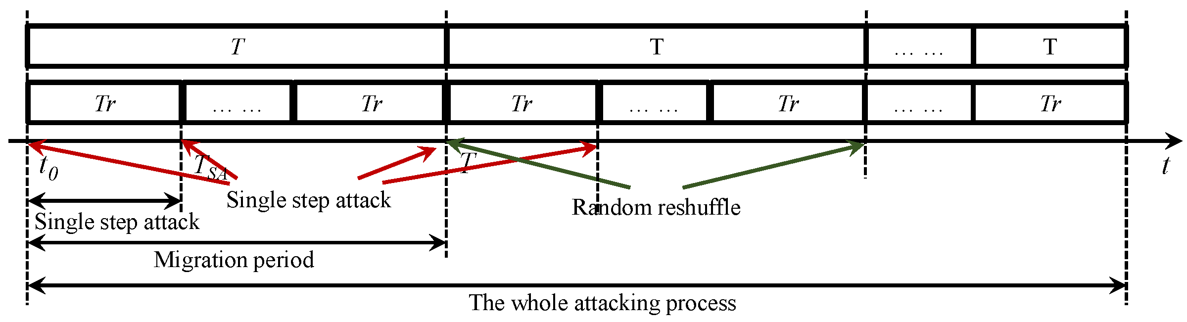
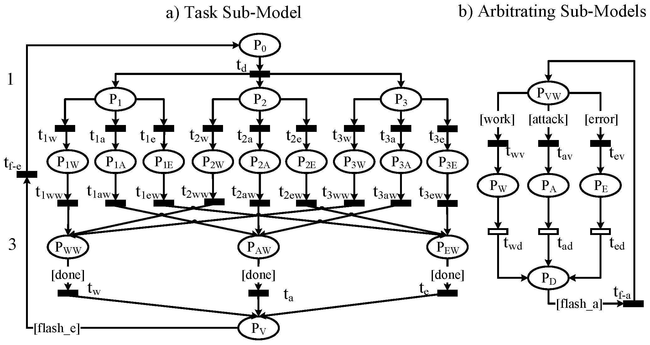
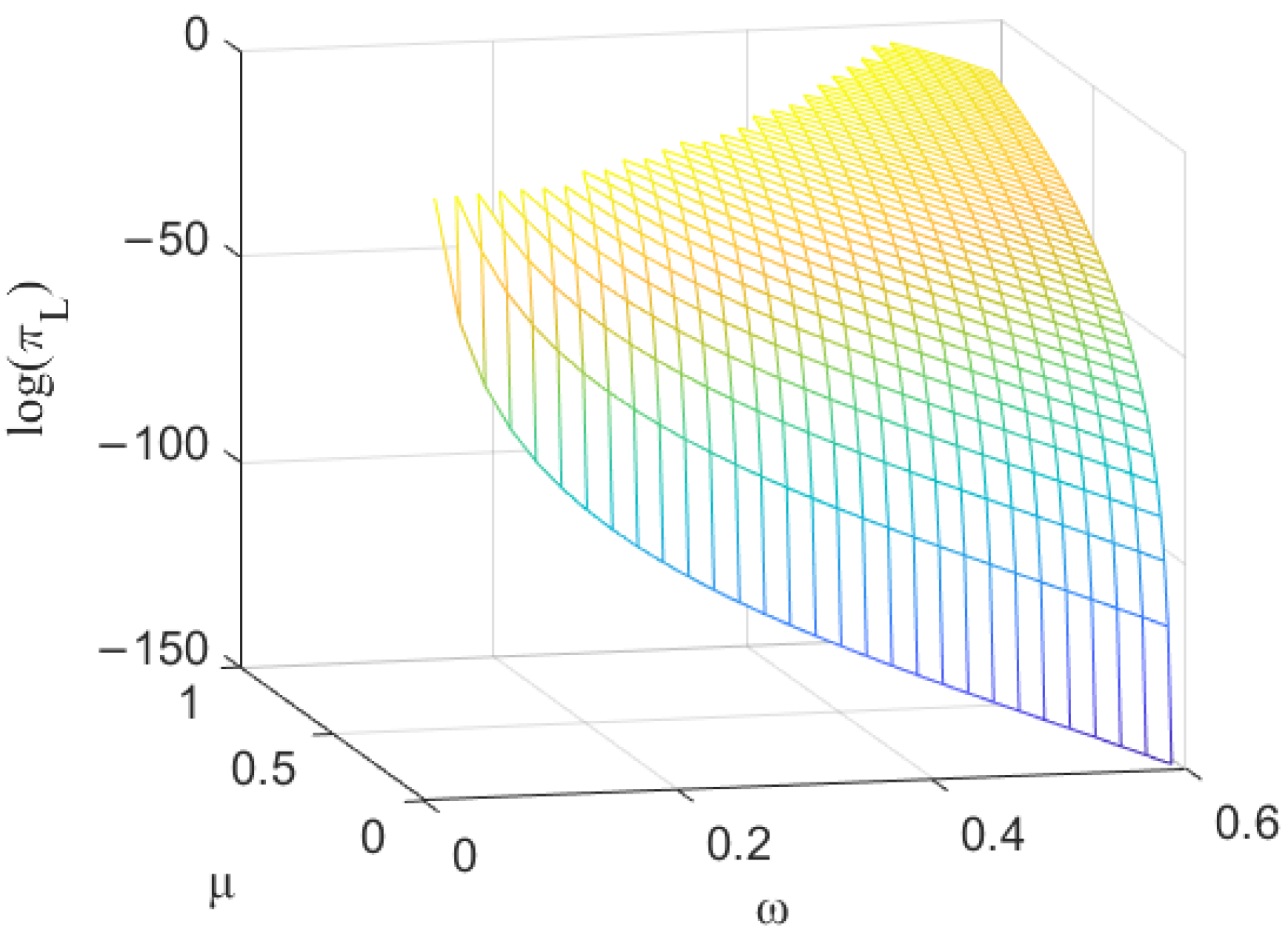
Table 1.
Summary of Notations.
| Variable | Description | |
|---|---|---|
| SRN model | N | A positive integer denoting the number of online SCVs |
| M | A positive integer indicating the output threshold, | |
| The being compromised probability of | ||
| The probability of compromising one node by an attack | ||
| The working probability of a node | ||
| Poisson model | r | Attack rate |
| The probability of compromising one node over each migration period | ||
| Markov Martingale | T | Migration period |
| The probability for each node to be migrated in every migration period | ||
| L | The length of attack chain | |
| The probability of node being compromised | ||
| Mean Time to Attack: the expected time until the attacker compromises his target () | ||
| Mean Time to Repair: the expected time until the attacker is being returned back to the entrance () |
Table 2.
Notation in the SRN.
| Notation | Description |
|---|---|
| The ACD node receives a task | |
| / | starts proceeding the task |
| / | executes the task in status |
| / | is attacked |
| / | There are some errors in |
| / | returns a result to the RMS and waits for arbitrating |
| / | returns a result to the RMS and waits for arbitrating |
| / | returns another result to the RMS and waits for voting |
| / | RMS finishes the vote |
| RMS is waiting for voting | |
| / | The x vector is arbitrated as the right one. The ACD node is in an x state |
| / | The arbitration is done |
| / | Flash and the next round |
Table 3.
Firing probabilities of transitions in the SRN.
| Transition | Firing Probability |
|---|---|
Table 4.
Guard functions of the SRN.
| Guard Function | Definition |
|---|---|
| if() return (1); else return (0); | |
| if( || ) return (1); else return (0); | |
| if(&& || ) return (1); else return (0); | |
| if(&& || || &&&&) return (1); else return (0); | |
| if() return (1); else return (0); | |
| if() return (1); else return (0); |
Table 5.
10 SCVs and Their Base Score.
| 1 | 2 | 3 | 4 | 5 | 6 | 7 | 8 | 9 | 10 | |
|---|---|---|---|---|---|---|---|---|---|---|
| BS | 5.8 | 6.0 | 7.5 | 5.0 | 9.3 | 6.8 | 5.0 | 7.5 | 10 | 4.3 |
Table 6.
Parameters used in the SRN.
| Name | Description | Parameter |
|---|---|---|
| The error probability of a SCV | 0.1 | |
| The compromising probability of a SCV | ||
| r | The single-step attack rate | /h |
| L | The length of attack chain | 30 |
Table 7.
Probabilities of a node being compromised and working.
| (3,2) | - | (3,3) | (4,3) | - | (4,4) | |||
| 0.6483 | 0.7164 | - | 0.2716 | 0.5838 | 0.4467 | - | 0.1147 | |
| 0.2517 | 0.1574 | - | 0.0156 | 0.3162 | 0.0951 | - | 0.0096 | |
| (5,3) | (5,4) | (5,5) | (6,4) | (6,5) | (6,6) | |||
| 0.524 | 0.5458 | 0.2130 | 0.0362 | 0.5508 | 0.4410 | 0.1573 | 0.0248 | |
| 0.376 | 0.2727 | 0.0649 | 0.0063 | 0.3492 | 0.1096 | 0.0190 | 0.0014 | |
| (7,4) | (7,5) | (7,7) | (8,5) | (8,6) | (8,8) | |||
| 0.5586 | 0.6282 | 0.3306 | 0.0157 | 0.6006 | 0.5960 | 0.3151 | 0.0163 | |
| 0.3414 | 0.1822 | 0.0473 | 0.2994 | 0.0559 | 0.0106 |
Table 8.
The number of reshuffled SCVs in each 100 h.
| (4,3) | (8,5) | (8,6) | (8,7) | (8,8) | |||
|---|---|---|---|---|---|---|---|
| 36.45 | 50.84 | 60.38 | 9.02 | 0 | 0 | ||
| 38.76 | 61.08 | 81.29 | 30.49 | 19.37 | 18.07 |
Publisher’s Note: MDPI stays neutral with regard to jurisdictional claims in published maps and institutional affiliations. |
© 2022 by the authors. Licensee MDPI, Basel, Switzerland. This article is an open access article distributed under the terms and conditions of the Creative Commons Attribution (CC BY) license (https://creativecommons.org/licenses/by/4.0/).
Share and Cite
MDPI and ACS Style
Yang, X.; Smahi, A.; Li, H.; Zhang, H.; Li, S.-Y.R. SPM: A Novel Hierarchical Model for Evaluating the Effectiveness of Combined ACDs in a Blockchain-Based Cloud Environment. Appl. Sci. 2022, 12, 9230. https://doi.org/10.3390/app12189230
AMA Style
Yang X, Smahi A, Li H, Zhang H, Li S-YR. SPM: A Novel Hierarchical Model for Evaluating the Effectiveness of Combined ACDs in a Blockchain-Based Cloud Environment. Applied Sciences. 2022; 12(18):9230. https://doi.org/10.3390/app12189230
Chicago/Turabian StyleYang, Xin, Abla Smahi, Hui Li, Huayu Zhang, and Shuo-Yen Robert Li. 2022. "SPM: A Novel Hierarchical Model for Evaluating the Effectiveness of Combined ACDs in a Blockchain-Based Cloud Environment" Applied Sciences 12, no. 18: 9230. https://doi.org/10.3390/app12189230
Note that from the first issue of 2016, this journal uses article numbers instead of page numbers. See further details here.