
A Study on the Freeze–Thaw Damage and Deterioration Mechanism of Slope Rock Mass Based on Model Testing and Numerical Simulation


1
Key Laboratory of Geotechnical Mechanics and Engineering of Ministry of Water Resources, Changjiang River Scientific Research Institute, Wuhan 430010, China
2
School of Civil Engineering and Architecture, Wuhan Polytechnic University, Wuhan 430023, China
*
Author to whom correspondence should be addressed.
Appl. Sci. 2022, 12(13), 6545; https://doi.org/10.3390/app12136545
Submission received: 9 June 2022
/
Revised: 20 June 2022
/
Accepted: 24 June 2022
/
Published: 28 June 2022
(This article belongs to the Special Issue Multiphysics Modeling for Fracture and Fragmentation of Geomaterials)
Abstract
:Engineering rock mass in cold regions has obvious freeze–thaw damage as a result of extreme differences in temperature, rainfall, snow, and other factors, which is one of the main causes of frequent geological disasters. Therefore, it is important to investigate the deterioration mechanism and evolution laws of rock mass freeze–thaw damage. Considering a hydropower station’s left bank slope in a cold region, model testing and numerical testing of slope rock mass failure under freeze–thaw conditions are here carried out by developing a generalized model. The results reveal that heat is transmitted from the outside to the inside of the slope and that the rate of temperature change varies with depth; the frost-heave force causes tensile cracks in the rock mass, with crack propagation taking the form of a circular arc; the presence of an original structural plane influences the propagation direction of the frost-heave crack, whereas the freezing rate of the fissure water influences the amplitude and growth rate of the frost-heave force. Additionally, a novel method of measuring frost-heave force is proposed. The largest frost-heave force caused by water–ice phase change is 19.3 kPa, which is equivalent to 3.17 MPa of the actual slope.
1. Introduction
In recent years, with the steady progress of China’s ‘western development’ strategy, a large number of water conservancy and hydropower projects, railways, highways, oil pipelines, and other engineering projects have been built in the western high-cold mountains. The frost damage to high and steep slopes, subgrades, tunnels, and building foundations poses a great challenge to the engineering construction and maintenance. The field of frozen soil mechanics has been studied for almost 70 years [1,2,3,4,5,6]. According to previous engineering experience, the formation of frozen soil is frequently accompanied by frozen rock issues, while the study of frozen rock is relatively new. Under the influence of periodic temperature changes for many years, the pore water in the rock mass has experienced repeated frost-heave and thaw-shrinkage processes. This also causes the original fractures inside the rock mass to continuously expand to a certain depth. Rock mass will be destroyed and degraded under varying temperatures and water content, resulting in geological disasters such as landslides [7,8,9,10,11,12]. According to the specific characteristics of rock slope engineering, it is necessary to carry out corresponding research on frozen rock mechanics. Here, the research status of freeze–thaw problems will be briefly introduced and analyzed. (1) In the investigation of the physical and mechanical properties of rock during the freeze–thaw cycle, Winkler et al. first pointed out that human research on frozen rocks began with the recognition of the frost heaving and thawing of ice in the 19th century. Frost heave, capillary water movement, and lithological variations are the main causes of freeze–thaw damage to rock masses [13]. Kostromitinov et al. analyzed the evolution law of the uniaxial compressive strength of rocks in different freeze–thaw temperature ranges [14]. Yamabe et al. conducted uniaxial and triaxial compression tests on sandstone under single freeze–thaw conditions at various temperatures, observing that frost-heave deformation in dry samples is elastic, whereas it is the opposite in saturated samples. Furthermore, freeze–thaw samples have a higher elastic modulus and higher compressive strength than unfrozen ones [15]. Yavuz et al. pointed out that the variation law of rock parameters after a freeze–thaw cycle is determined by the initial state and porosity of the rock [16]. Khanlari et al. assessed the long-term durability of Iranian red sandstone after 30 freeze–thaw cycles and proposed that the distribution law of pores plays a significant role in the degree of freeze–thaw damage in red sandstone [17]. Ghobadi et al. considered Brazilian tensile strength to be a critical criterion for determining the durability of freeze–thaw rocks [18]. Momeni et al. carried out 300 freeze–thaw cycles on granites from three different origins, compared and analyzed the evolution laws of various physical and mechanical parameters, and concluded that the longitudinal wave velocity is the best index for evaluating the physical and mechanical properties of freeze–thaw granite [19]. The impacts of freeze–thaw cycles on the physical and mechanical properties of some sedimentary rocks in Turkey were investigated by Sarici et al. The freeze–thaw cycle causes sample porosity to rise while decreasing point load strength, Schmidt hardness, and weight. The point load strength loss and the Schmidt hardness loss have a strong relationship after 20 cycles, which is highly useful for estimating the point load strength following freeze–thaw cycles [20]. In brief, the main trends in the research on the physical and mechanical properties of rock freeze–thaw are as follows: The freeze–thaw cycle treatment methods change from a single freeze–thaw cycle and a single temperature gradient to different cycles and different temperature gradients. The test method has progressed from the uniaxial compression test to the conventional triaxial compression test and then to the triaxial compression unloading and creep tests. The research content has developed from simple static characteristics to complex dynamic characteristics. (2) The mechanism of rock freeze–thaw damage, rock freeze–thaw damage is caused by the combined action of volume expansion caused by water–ice phase change and ice segregation caused by water migration. The mechanism is often studied by microscopic means. The effect of critical saturation and pore-size distribution in freezing injury was investigated by Al-Omari. The findings suggest that first and foremost, freeze–thaw failure will occur even after a few freeze–thaw cycles when the saturation of the two types of limestone investigated surpasses 80–85%. The freezing effect is quite quick if the water saturation is sufficient. The critical saturation of these rocks is the same, notwithstanding the differences in porosity. Finally, increasing the number of freeze–thaw cycles has no influence on critical saturation; rather, the pore-size distribution, rather than total porosity, controls the freezing damage. The critical saturation, it is stated, can be described as the fundamental features of stone [21]. Martínez-Martínez et al. studied the freeze–thaw resistance of rocks as well as their physical evolution during weathering. The crack initiation, propagation, and fracture processes during the freeze–thaw cycle were observed by microscopic observation. The spatial attenuation of ultrasonic waves was discovered to be the most sensitive parameter for detecting the critical attenuation threshold of rock and its imminent fracture. The standardized durability test cannot accurately reflect the reality of rock frost weathering. It is suggested that the number of freeze–thaw cycles be increased and that the weathering process of samples be monitored using ultrasonic measurement [22]. De Argandona et al. imaged the texture characteristics and internal void structure of dolomitic rocks using X-ray computed tomography. X-ray CT was used to study the evolution of pore structure during the freeze–thaw cycle test. The images obtained can be used to track the progressive decay and evaluate the internal depth of damage, and damage was observed primarily in the form of cracks [23]. Ruedrich et al. carried out a long-term experimental study of over 1400 freeze–thaw cycles on four selected rocks. The samples in the freeze–thaw test were affected by changes in temperature and moisture, indicating that different decay mechanisms may interfere with each other. Thermohygric and moisture expansion were mentioned as important damage processes [24]. (3) The numerical simulation of rock freezing and thawing: Davidson et al. prefabricated open single-fracture rock samples, injected water into the fractures, conducted frost-heave tests, and measured the frost-heave force. Based on this, a two-dimensional finite element model was established, and the numerical solution of the frost-heave force was calculated using the equivalent thermal expansion coefficient [25]. Rode et al. pointed out that the rock moisture in the freezing and thawing process is the key factor in frost weathering. They extrapolated the water content information for natural rock walls from other relevant knowledge and integrated it into the WUFI® software package to simulate the freezing–thawing and weathering mechanisms of natural rock walls related to water [26]. Yahaghi et al. used the in-house three-dimensional mixed finite element code to study the failure mechanism of Tasmanian sandstone subjected to different freeze–thaw cycles in UCS and BTS tests. The three-dimensional numerical simulation shows that for the model both with and without freeze–thaw cycles, the final failure occurs in the central part, but with the increase in the number of freeze–thaw cycles, the failure surface becomes more tortuous [27]. Neaupane et al. developed a numerical model of a thermal–mechanical–fluid flow coupling system and used it to simulate the freezing and thawing of rocks, taking into account pore water phase change during the freezing process. Temperature transfer and deformation behavior can be well predicted in the limit range of elastic deformation. However, irreversible and plastic effects cannot be taken into account [28]. Neaupane et al. further created a nonlinear elastoplastic simulation program for rock freezing and thawing. The Mohr–Coulomb failure criterion is assumed to be valid for yield locus and plastic potential. The program’s prediction of temperature transfer and deformation agrees well with the results of the freeze–thaw test [29].
Numerous investigations into physical and mechanical rock freeze–thaw testing at the sample level have been conducted, and various methods for measuring frost-heave force and distinguishing rock frost-heave phases have been proposed. Physical model experiments of medium and large-scale rock mass damage and failure under freeze–thaw conditions, on the other hand, are rarely conducted. In the aspect of numerical simulation, the study results generally focus on the solution of frost-heave force and the distribution of stress fields in the model, while the research on the initiation and propagation process of frost-heave crack is comparatively limited.
Relying on a water conservancy project in the cold region of China, the minimum temperature in the dam site area of the project for many years has been −45 °C, the maximum temperature is 36.6 °C, and the extreme temperature difference is more than 80 °C, which places high requirements on a freeze–thaw damage study of high and steep slopes with such an extreme temperature difference. Next, the physical model test and numerical simulation of the dam site slope will be carried out to explore the evolution law of frost-heave failure of slope rock mass under the freeze–thaw conditions. The main contents of the research are as follows: (a) Using the similarity theorem, the similarity criterion and similarity ratio of a freeze–thaw test of a rock mass are derived, and a physical model of a cracked slope rock mass is built. The freeze–thaw cycle test is then used to investigate the variation laws of the temperature field, fissure water pressure, and frost-heave deformation of the model slope. (b) The numerical model of the slope is established using RFPA2D-thermal software to analyze the frost-heave failure mode and crack propagation law of an ice-containing fractured slope.
2. Physical Model Testing of Freeze–Thaw Damage and the Deterioration Mechanism of Slope Rock Mass
Taking a slope on the left bank of the dam site of the aforementioned hydropower station as a prototype, we select appropriate similar materials, build an indoor scale model, carry out a large-scale physical model test of slope rock mass failure under freeze–thaw conditions, and conduct related research.
2.1. Design of Physical Model of Freeze–Thaw Slope
Shown in Figure 1 is the engineering geological map of the left bank slope of the power station. The slope’s shallow layer is composed of class IV rock mass, while the upper portion is composed of class III rock mass, and the deep portion is composed of class II rock mass. The elevation of the left bank slope is 800~980 m. In the upper and lower parts, two weak interlayers, f2 and f3, are developed. The BQ classification is used to classify the quality of the rock mass. In this case, the prototype slope is generalized as a right triangle slope with a height of 180 m and a bottom length of 200 m. The indoor scale model is established with a geometric similarity constant of 100. As shown in Figure 2, the scale model is 1.8 m high, 2.0 m long, and 0.40 m wide. Obviously, the connection between f2 and f3 under the condition of a freeze–thaw cycle will seriously affect the stability of the slope.
2.2. Determining Similar Materials
Because the weak interlayer is located in class III rock mass, determining the physical and mechanical properties of this rock mass will be crucial to the development of this physical model. The parameters of the class III rock mass are comprehensively determined according to the in situ field testing and the field rock mass quality classification carried out for the above-mentioned project.
In order to make the parameters of similar materials meet the similarity theory and reproduce the freeze–thaw failure process indoors, gypsum and water are selected as raw materials to simulate the rock mass. According to the above quasi rock mass physical and mechanical parameters, after many tests, the mixture ratio of model material is determined as gypsum:water = 1:0.7. Table 1 provides the main physical and mechanical parameters of model materials corresponding to this mixture ratio. Since the class II rock mass is mostly distributed below the fault and is less affected by the freeze–thaw cycle, the mixture ratio of class II rock mass model material is set as 1:0.6. As the texture of class IV rock mass is relatively loose, some stacked gypsum precast blocks with a mixture ratio of 1:0.6 are selected to represent it. The size of the precast block is 240 mm long, 115 mm wide, and 53 mm high. The material of the weak interlayer f2 is simulated by the high molecular water-absorbing resin, its cohesion is c = 1 kPa, and its internal friction angle is φ = 13°. The weak interlayer f3 is a prefabricated crack with a width of 1 cm, and the crack surface is pasted with polyethylene film for waterproofing. During the test, water is filled into the weak interlayer to simulate the water–ice phase change process when the water content is high.
To verify whether the physical and mechanical properties of the model materials meet the basic requirements of similar materials, the following similarity constant relationship is established in combination with similarity theory:
where Cσ is the stress similarity constant; Cγ is the unit weight similarity constant; CL is the geometric similarity constant; Cε is the strain similarity constant; Cf is the similarity constant of the internal friction angle; Cμ is the Poisson’s ratio similarity constant; CE is the deformation modulus similarity constant; Cc is the cohesion similarity constant; and CRc is the compressive strength similarity constant.
Table 2 shows the actual and theoretical similarity constants. The physical and mechanical properties of the model material basically meet the similarity constant relationship, and the small deviation in the similarity relationship does not affect the qualitative analysis of the test results. The material can be used to simulate the prototype slope to preliminarily explore its freeze–thaw failure law.
2.3. Test System of the Freeze–Thaw Simulation
The test was carried out in the large cold storage unit of the geomechanical model laboratory of Changjiang River Scientific Research Institute, which includes two parts: the test system inside the storage unit and the monitoring system outside the storage unit. The size of the cold storage unit is 6 m × 3 m × 3.3 m, the adjustable temperature range is 30~−20 °C, and the design cooling rate is 20~30 °C/h, as shown in Figure 3a. The storage unit body is made of polyurethane double-sided colored steel plate and hard polyester foam plastic, which has stable thermal conductivity and good durability. Stiff foam polyurethane composite insulation board is used to build the insulation box, which isolates the model from the outside on all four sides. The joints are plugged with foaming agent to imitate the heat transmission from the slope’s surface to its inside. Figure 3b shows the insulation box.
2.4. Monitoring System for Temperature, Displacement and Frost-Heave Force
A total of 7 temperature sensors T1~T7 are set at depths 5 cm, 10 cm, 15 cm, 20 cm, 25 cm, 30 cm, and 35 cm from the slope surface, as shown in Figure 4. Displacement sensors L1, L3, L5, and L7 measure the vertical displacement of the slope surface, whereas displacement sensors L2, L4, L6, and L8 measure the horizontal displacement of the slope surface. A micro-osmometer S1 is placed at the bottom of the simulated weak interlayer f3.
2.5. Procedures of Freeze–Thaw Test
The freeze–thaw test was performed in three steps: (a) trial produce and purchase similar materials; (b) fabricate the gypsum block mold and the model template; (c) pour the mold, remove the formwork, and embed the temperature sensors during pouring; (d) install and debug the osmometer, displacement sensor, and camera system; (e) assemble the insulation room and seal the joints; (f) and start the freeze–thaw test by injecting water into the f3. The data were then collected, recorded, and observed.
The data to be collected and recorded in the test process included temperature, deformation, pressure, crack opening width, crack development law, and slope failure process. Every minute, the temperature, deformation, and osmotic pressure were recorded; picture data were collected every 30 min; and the camera system captured the entire freeze–thaw test procedure. During this period, the acquisition frequency was modified as needed to match the current condition.
3. Analysis of Physical Model Test Results
The test experienced a freeze–thaw cycle that lasted 180 h. The evolution rules of temperature field, deformation, and frost-heave force in the slope were investigated in detail based on the test monitoring results.
3.1. Temperature Field Analysis of Freeze–Thaw Rock Mass
Figure 5 shows the law of temperature change at measuring points at different depths during the freeze–thaw cycle. During the cooling process, it was discovered that: (a) the temperature in the cold storage drops to around −13 °C within 20 h and then fluctuates slightly, with a fluctuation range of ±2 °C; (b) the temperature curves at different depths exhibit essentially the same drop law during the cooling process, showing that heat is uniformly transmitted to the outside; (c) the temperature evolution law at the slope surface and the slope buried depth of 8 cm is very similar to that in cold storage. However, the temperature of the measuring point at the buried depth of 24 cm decreases slowly, falling to just about 0 °C after 120 h. The temperature change of the measuring points with a buried sensor depth of 24~32 cm presents a smooth curve and is not sensitive to the fluctuation of indoor temperature. It can be seen that with the increase in buried depth, the influence of external temperature changes on the interior of the rock mass will be weaker, and the cooling rate will also slow down. (d) Affected by the latent heat of pore water in the model, when the slope surface temperature drops to 0 °C, the temperature curve will have a plateau period of about 25 h before continuing to decline. In the heating process, (a) the change rate of indoor temperature changes from fast to slow, and the slope of the corresponding time-varying curve changes from large to small; (b) the response of slope body temperature lags far behind, and slope body must be preheated for an extended period of time. Using the slope surface as an example, it takes approximately 28 h, and the interior of the slope body takes even longer; (c) the heating rate will accelerate after the slope has been preheated, and the trend will be linear.
3.2. The Progressive Failure Process of Freeze–Thaw Slope Rock Mass
Figure 6 shows the curves of temperature change, frost-heave force, and slope surface displacement of the model slope during the cooling process. The deformation experienced four stages: frost-heave incubation, frost-heave initiation, frost-heave development, and crack propagation. Frost-heave incubation stage: The temperature on the slope surface drops from 25 °C to −7 °C. The fissure water is still liquid at this point, and the stored latent heat is continuously released. As a result, the horizontal and vertical displacement of the slope surface remain constant after a period of fluctuation, and the frost-heaving phenomenon is not obvious. Frost-heave initiation stage: The temperature on the slope surface continues to fall, while the displacement of the L2 measuring point on its upper part increases steadily. The water in the upper section of the fracture freezes at this point, forming an ice plug. As the unfrozen water in the lower part is strictly sealed, the excess hydrostatic pressure is gradually generated under the continuous pressure of the ice plug. It reduces immediately when the osmometer value increases to 7.8 kPa. The reason for this is that after the frost-heave initiation, the frost-heave power is released owing to newly formed microscopic cracks in the weak areas of the rock mass, but the material as a whole retains its ability to bear the load. Frost-heave development stage: The slope surface temperature is maintained at −13 °C, the freezing rate of fissure water increases, and the unfrozen water content falls. Because the frost-heave force develops rapidly after the ice jam effect forms, the osmometer measurement quickly rises to 19.3 kPa. The frost-heave force, temperature field, and slope deformation all maintain a rather balanced state over time, increasing progressively until they reach their peak. Furthermore, the upper part of the slope surface’s horizontal displacement continues to rise, and the upper part’s frost-heave force compresses the lower masonry, resulting in two stepped increases in the slope bottom’s horizontal displacement. Crack propagation stage: The frost-heave force will squeeze the crack tip through the unfrozen water in the lower part. When the driving force of crack propagation is reached, the crack tip expands, and the frost-heave force is released instantly. According to the monitoring results, the maximum frost-heave force is 19.3 kPa. Because the model’s stress similarity constant is 164, the prototype slope’s frost heave force can be calculated to be 3.17 MPa. The class III rock mass has cohesion of 0.7 to 1.5 MPa, and the frost-heave force generated is sufficient to cause freeze–thaw damage.
Figure 7 shows the osmometer values, slope deformation, and temperature change curves during the heating process of the freeze–thaw cycle. As the temperature rises, the value of the osmometer decreases until it eventually fluctuates around the hydrostatic pressure of roughly 2.2 kPa. Meanwhile, the solid ice melts into liquid water, and the L2 and L7 measuring locations experience 0.2 mm and 0.4 mm of shrinkage deformation, respectively. Other measuring points do not seem to be deformed.
The deformation form of the model slope after one freeze–thaw cycle is shown in Figure 8. A crack was formed at the bottom of the weak interlayer f3 due to frost-heave force. The crack propagates to the lower right side first, then develops into an arc to the lower left side. The crack turns to the rock mass’s sliding direction under the influence of the rock mass’s self-weight. The crack propagation depth is approximately 6 cm, and the crack tip is close to the model boundary.
The second freeze–thaw cycle has yet to begin, and crack f3 extends and cuts through the entire upper rock mass. The rock mass staggered due to self-weight and pushed the lower rock mass to slide, resulting in a landslide. Figure 9 shows the slope shape after instability. It should be noted that the model test simulates the ideal state in which the crack f3 is completely filled with water and the crack penetration path is short, making the crack more prone to deformation under the action of frost-heave force. The actual environment of the slope rock mass is more complex and requires additional research.
4. Numerical Simulations of Frost-Heave Failure of the Slope Rock Mass
Because the physical model test cannot reveal the changes in the model’s internal stress state, the prototype slope is first simplified into a numerical model including a crack and a weak interlayer; then, the numerical simulation is used to study the distribution of the internal stress field, the evolution process of the frost-heave force, and the crack propagation of the slope rock mass, in order to reveal the damage and deterioration mechanism.
4.1. Foundations of RFPA2D-Thermal
The two-dimensional finite element software RFPA2D-Thermal uses elasticity for the stress analysis and establishes the element failure analysis system based on the theory of elastic damage mechanics and the modified Coulomb failure criterion. Its theoretical basis and software architecture were initially proposed by Professor Tang’s team and further developed by Mechsoft. RFPA2D-Thermal has been successfully applied to the study of the temperature effects of rock and concrete [30,31].
In the temperature–stress coupling problem, the total strain of the material is:
where εe is the strain caused by stress and εT is the strain caused by temperature.
Temperature strain εT is related to the temperature expansion of the material, which can be expressed as
where is the thermal expansion coefficient of the material; T is the current temperature; and T0 is the initial temperature.
The temperature–stress coupling constitutive relationship of the material is
where and are Lame’s constants, and , .
4.2. Numerical Model of a Slope with an Ice Crack
The numerical model of the slope, as shown in Figure 10, is 180 m high and 200 m wide, with 3,600,000 elements. The slope model’s left and lower sides are adiabatic boundaries that constrain displacement in the horizontal and vertical directions, respectively, and the slope surface is a free and heat-transfer boundary. The precast crack f3 is 40 m × 1 m in dimension and is filled with ice. The model’s initial temperature is 0 °C, with a temperature load increment of −1 °C at the heat transfer boundary. The numerical simulation is divided into 20 steps, each lasting 1 h. The thermodynamic and physical and mechanical parameters of the rock mass and ice are shown in Table 3 and Table 4, respectively. To study the stress distribution of a heterogeneous rock mass under the action of frost-heave force, the calculation element in RFPA2D-thermal is endowed with heterogeneous characteristics. The parameters of each calculation element are assumed to follow the Weibull distribution. The homogeneity parameter U controls the parameter’s nonuniformity; the smaller the U value, the stronger the material’s nonuniformity. After multiple trial calculations, the final crack growth is comparable with the actual scenario when the homogeneity is U = 3.
4.3. The Analysis of the Stress and Crack Propagation Law of the Slope Rock Mass under Negative Temperature
In view of the lack of relevant physical and mechanical parameters of class II rock mass and considering that the deep rock mass is less affected by temperature, class II and III temporarily take the same parameters shown in Table 1. The physical and mechanical parameters of quartz schist suffering 25 indoor freeze–thaw cycles are determined as the parameters for class IV. The physical and mechanical parameters of the filling medium in the weak interlayer f2 are obtained from the field test, as shown in Table 5.
Figure 11 shows the slice stress distribution curve and the minimum principal stress distribution diagram at each typical time. The slices are cut along the left, middle, and right sides of f3, with line A, line B, and line C as the corresponding cutting lines. Because the calculation elements behind element 70 are so far from f3 and the influence of frost expansion is so minor, each drawing only presents the distribution curve of the minimum principal stress σ3 for the first 70 elements. Figure 11b shows the distribution of the model’s minimum principal stress when a −5 °C temperature load is applied to the slope surface. Because each element is heterogeneous, the stress around f3 vibrates under the drive of frost-heave force, and the tensile stress of elements 30–40 at the bottom of f3 is concentrated. The model’s stress contour also shows that there is a tensile stress zone (shown in white) at the bottom of the ice-containing crack f3, and the element stress response of line C is earlier than those of line A and line B. When the temperature load on the slope surface is maintained at −10 °C, the frost-heave force begins to damage the rock mass around the crack f3, as illustrated in Figure 11c. At the bottom of the crack, some failure elements develop, and the crack progressively expands to the slope’s surface. The element tensile stress increases near the slope surface at the bottom of crack f3. Figure 11d shows that when the temperature drops, the oscillation amplitude of the minimum principal stress on both sides of f3 increases, and tensile stress zones develop in many locations. The frost-heave crack at the bottom continues to develop and gradually develops downward. It has a connecting trend with the weak interlayer f2, and the failure surface is initially formed. When the temperature drops further, the bottom of crack f3 extends downward, joins with f2 to form a linked crack, and then gradually expands along the weak interlayer f2, as shown in Figure 11e.
To summarize, the water stored in the cracks or weak interlayers of the rock slope undergoes a water–ice phase change under negative temperature conditions. The frost-heave force is generated at this point when the volume of the ice expands but is confined by the surrounding rock mass. The rock mass is microcracked when the frost-heave force exceeds the crack propagation threshold value. The nearby weak interlayer and fracture zone connect to each other when frost-heave damage accumulates, severely reducing the slope’s stability and resulting in geological disasters such as landslides and collapses.
4.4. Influence of Fissure Water Freezing Rate on Damage and Deterioration of Slope Rock Mass under Negative Temperature
The freezing rate of fissure water is a main factor affecting the frost-heave failure of fractured rock mass. Four slope models with various fissure water freezing rates have been constructed, which are 25%, 50%, 75%, and 100%, respectively; the equivalent thermal expansion coefficients are, respectively, −37.5, −75.0, −112.5, and −150.0. Figure 12 shows the distribution of the model’s minimum principal stress after 20 h of frost-heave expansion. The tensile stress zone is initiated at the bottom of the crack, accompanied by a small number of failure elements when the freezing rate of the fissure water is 25%. There is no further crack growth due to the small frost-heave force. The final crack propagation mode of the rock mass with 50%, 75%, and 100% fissure water freezing rates is essentially the same. However, as the freezing rate increases, the crack propagation length increases, and the model’s maximum tensile stress decreases.
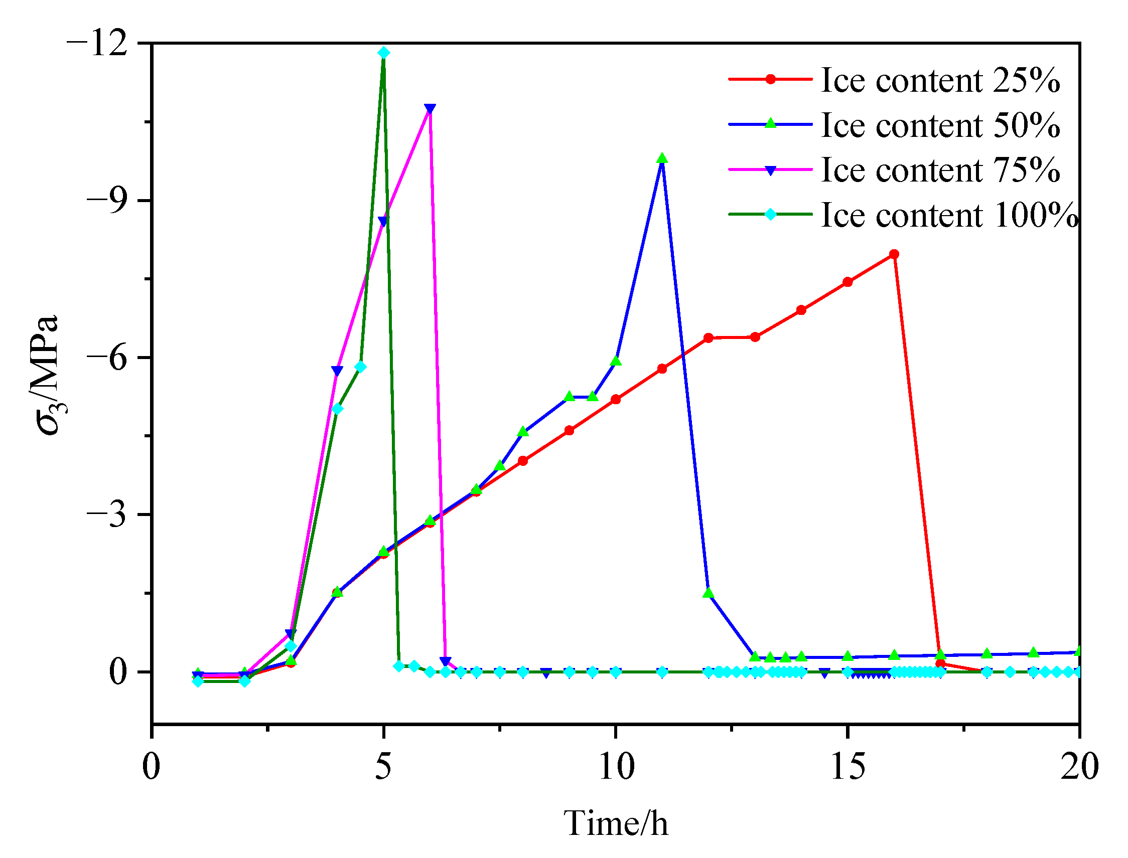
In order to study the evolution process of the tensile stress at the bottom of the fracture, the minimum principal stress σ3 of the calculation element at the bottom of the crack f3 under different water freezing rates is extracted, as shown in Figure 13. The time it takes to generate tensile stress is not affected by the freezing rate of the fissure water, and it takes about 3 h. The time required for the tensile stress to reach their respective peaks decreases continuously as the freezing rate increases, and the corresponding peak stress increases.
It can be concluded that the water content of fractures or weak interlayers has a significant impact on the stability of a rock slope. When the water content of the fracture is low, as in the current study, cooling has no influence on slope stability. When the freezing rate of fissure water reaches a particular level, frost-heave forces demolish the weak component of the rock mass. The geometry of crack propagation changes little as the freezing rate rises, but it has a considerable impact on the magnitude of frost-heave force and its growth rate.
5. Conclusions
Model testing of the failure of steep fractured rock mass under freeze–thaw conditions is carried out using the left abutment slope of a hydropower station as the prototype. Under the freeze–thaw cycle, the evolution rules of the temperature field, slope deformation, frost-heave force, and macroscopic deformation features of the slope are investigated. Numerical simulations are used to investigate the rules of fracture propagation and the effects of freezing rates on slope deterioration. The following are the main conclusions.
The heat is transmitted from the outside to the inside of the slope. The rate of temperature change varies depending on depth; the closer to the surface, the faster the rate of change, and the shape of the temperature curve is closest to the air temperature. The temperature change rate is slower and the temperature curve is smoother farther away from the slope surface.
Within the cold storage unit’s temperature range, it is evident that unfrozen water is always present at the bottom of the crack during the cooling process; thus, a strategy for inserting an osmometer in the unfrozen water to measure the frost-heave force is designed. During the cooling process, the osmometer’s reading rises in a fluctuating manner. The water–ice phase change produces a small amount of frost-heave power. The osmometer’s maximum reading is 19.3 kPa, which is equal to 3.17 MPa for the prototype slope frost-heave force. This test also presents a new way to measure frost-heave force.
The steep fracture opens to the free side during the cooling process due to the frost-heave force induced by water–ice phase change. During the heating process, the cracks are subjected to shrinkage deformation due to solid ice melting. The crack tip expands when the frost-heave force reaches a certain value, and the crack propagation shape is mainly a circular arc. When the intact rock mass’s strength is insufficient to withstand the sliding force, the rock mass continues to expand along the potential sliding direction until an independent sliding body is formed.
The numerical simulation results reveal that under the action of frost-heave force, the tensile stress at the crack tip is concentrated, and crack initiation occurs when the tensile stress reaches the tensile strength of the rock mass. The crack grows further into the rock mass as the temperature drops, resulting in a connection between the original crack and the weak interlayer, forming a large sliding plane and eventually causing a landslide disaster.
Author Contributions
Conceptualization, J.Z. and D.X.; methodology, J.Z.; software, B.W.; validation, J.Z., D.X. and B.W.; formal analysis, J.Z.; investigation, C.L.; resources, J.Z.; data curation, C.L.; writing—original draft preparation, J.Z.; writing—review and editing, D.X.; visualization, B.W.; supervision, B.W.; project administration, B.W.; funding acquisition, J.Z. All authors have read and agreed to the published version of the manuscript.
Funding
This study was supported by the National Natural Science Foundation of China (Nos. 41877280, 12072047) and the National Key R&D Program of China (No. 2018YFC0407002).
Institutional Review Board Statement
Not applicable.
Informed Consent Statement
Not applicable.
Data Availability Statement
Not applicable.
Conflicts of Interest
The authors declare no conflict of interest.
References
- Henry, H.A.L. Soil freeze–thaw cycle experiments: Trends, methodological weaknesses and suggested improvements. Soil Biol. Biochem. 2007, 39, 977–986. [Google Scholar] [CrossRef]
- Congreves, K.A.; Wagner-Riddle, C.; Si, B.C.; Clough, T.J. Nitrous oxide emissions and biogeochemical responses to soil freezing-thawing and drying-wetting. Soil Biol. Biochem. 2018, 117, 5–15. [Google Scholar] [CrossRef]
- Smith, N.V.; Saatchi, S.S.; Randerson, J.T. Trends in high northern latitude soil freeze and thaw cycles from 1988 to 2002. J. Geophys. Res.-Atmos. 2004, 109, D12101. [Google Scholar] [CrossRef]
- Freppaz, M.; Williams, B.L.; Edwards, A.C.; Scalenghe, R.; Zanini, E. Simulating soil freeze/thaw cycles typical of winter alpine conditions: Implications for N and P availability. Appl. Soil Ecol. 2007, 35, 247–255. [Google Scholar] [CrossRef]
- Kreyling, J.; Beierkuhnlein, C.; Pritsch, K.; Schloter, M.; Jentsch, A. Recurrent soil freeze–thaw cycles enhance grassland productivity. New Phytol. 2008, 177, 938–945. [Google Scholar] [CrossRef]
- Edwards, L.M. The effects of soil freeze–thaw on soil aggregate breakdown and concomitant sediment flow in Prince Edward Island: A review. Can. J. Soil Sci. 2013, 93, 459–472. [Google Scholar] [CrossRef]
- Shin, Y.; Choi, J.C.; Quinteros, S.; Svendsen, I.; L’Heureux, J.; Seong, J. Evaluation and monitoring of slope stability in cold region: Case study of man-made slope at Øysand, Norway. Appl. Sci. 2020, 10, 4136. [Google Scholar] [CrossRef]
- Gowthaman, S.; Iki, T.; Nakashima, K.; Ebina, K.; Kawasaki, S. Feasibility study for slope soil stabilization by microbial induced carbonate precipitation (MICP) using indigenous bacteria isolated from cold subarctic region. SN Appl. Sci. 2019, 1, 1480. [Google Scholar] [CrossRef] [Green Version]
- Mufundirwa, A.; Fujii, Y.; Kodama, N.; Kodama, J. Analysis of natural rock slope deformations under temperature variation: A case from a cool temperate region in Japan. Cold Reg. Sci. Technol. 2011, 65, 488–500. [Google Scholar] [CrossRef] [Green Version]
- Ballantyne, C.K.; Stone, J.O. Timing and periodicity of paraglacial rock-slope failures in the Scottish Highlands. Geomorphology 2013, 186, 150–161. [Google Scholar] [CrossRef]
- Krautblatter, M.; Funk, D.; Günzel, F.K. Why permafrost rocks become unstable: A rock–ice-mechanical model in time and space. Earth Surf. Proc. Land. 2013, 38, 876–887. [Google Scholar] [CrossRef] [Green Version]
- Murton, J.B.; Peterson, R.; Ozouf, J.C. Bedrock fracture by ice segregation in cold regions. Science 2006, 314, 1127–1129. [Google Scholar] [CrossRef] [PubMed] [Green Version]
- Winkler, E.M. Frost damage to stone and concrete: Geological considerations. Eng. Geol. 1968, 2, 315–323. [Google Scholar] [CrossRef]
- Kostromitinov; Nikolenko, K.N.; Nikitin, B.D. Testing the strength of frozen rocks on samples of various forms. In Increasing the effectiveness of mining industry in Yakutia. Int. J. Rock Mech. Min. Geomech. Abstr. 1974, 12, 32–37. [Google Scholar]
- Yamabe, T.; Neaupane, K.M. Determination of some thermo-mechanical properties of Sirahama sandstone under subzero temperature condition. Int. J. Rock Mech. Min. 2001, 38, 1029–1034. [Google Scholar] [CrossRef]
- Yavuz, H.; Altindag, R.; Sarac, S.; Ugur, I.; Sengun, N. Estimating the index properties of deteriorated carbonate rocks due to freeze–thaw and thermal shock weathering. Int. J. Rock Mech. Min. 2006, 43, 767–775. [Google Scholar] [CrossRef]
- Khanlari, G.; Sahamieh, R.Z.; Abdilor, Y. The effect of freeze–thaw cycles on physical and mechanical properties of Upper Red Formation sandstones, central part of Iran. Arab. J. Geosci. 2015, 8, 5991–6001. [Google Scholar] [CrossRef]
- Ghobadi, M.H.; Taleb Beydokhti, A.R.; Nikudel, M.R.; Asiabanha, A.; Karakus, M. The effect of freeze–thaw process on the physical and mechanical properties of tuff. Environ. Earth Sci. 2016, 75, 846. [Google Scholar] [CrossRef]
- Momeni, A.; Abdilor, Y.; Khanlari, G.R.; Heidari, M.; Sepahi, A.A. The effect of freeze–thaw cycles on physical and mechanical properties of granitoid hard rocks. Bull. Eng. Geol. Environ. 2016, 75, 1649–1656. [Google Scholar] [CrossRef]
- Sarici, D.E.; Ozdemir, E. Determining point load strength loss from porosity, Schmidt hardness, and weight of some sedimentary rocks under freeze–thaw conditions. Environ. Earth Sci. 2018, 77, 62. [Google Scholar] [CrossRef]
- Al-Omari, A.; Beck, K.; Brunetaud, X.; Török, Á.; Al-Mukhtar, M. Critical degree of saturation: A control factor of freeze–thaw damage of porous limestones at Castle of Chambord, France. Eng. Geol. 2015, 185, 71–80. [Google Scholar] [CrossRef]
- Martínez-Martínez, J.; Benavente, D.; Gomez-Heras, M.; Marco-Castaño, L.; Ángeles García-del-Cura, M. Non-linear decay of building stones during freeze–thaw weathering processes. Constr. Build. Mater. 2013, 38, 443–454. [Google Scholar] [CrossRef]
- De Argandona, V.G.R.; Rey, A.R.; Celorio, C.; Suárezdel Río, L.M.; Calleja, L.; Llavona, J. Characterization by computed X-ray tomography of the evolution of the pore structure of a dolomite rock during freeze–thaw cyclic tests. Phys. Chem. Earth Part A Solid Earth Geod. 1999, 24, 633–637. [Google Scholar] [CrossRef]
- Ruedrich, J.; Kirchner, D.; Siegesmund, S. Physical weathering of building stones induced by freeze–thaw action: A laboratory long-term study. Environ. Earth Sci. 2011, 63, 1573–1586. [Google Scholar] [CrossRef] [Green Version]
- Davidson, G.P.; Nye, J.F. A photoelastic study of ice pressure in rock cracks. Cold Reg. Sci. Technol. 1985, 11, 141–153. [Google Scholar] [CrossRef]
- Rode, M.; Schnepfleitner, H.; Sass, O. Simulation of moisture content in alpine rockwalls during freeze–thaw events. Earth Surf. Proc. Land. 2016, 41, 1937–1950. [Google Scholar] [CrossRef]
- Yahaghi, J.; Liu, H.; Chan, A.; Fukudaab, D. Experimental and numerical studies on failure behaviours of sandstones subject to freeze–thaw cycles. Transp. Geotech. 2021, 31, 100655. [Google Scholar] [CrossRef]
- Neaupane, K.M.; Yamabe, T.; Yoshinaka, R. Simulation of a fully coupled thermo–hydro–mechanical system in freezing and thawing rock. Int. J. Rock Mech. Min. 1999, 36, 563–580. [Google Scholar] [CrossRef]
- Neaupane, K.M.; Yamabe, T. A fully coupled thermo-hydro-mechanical nonlinear model for a frozen medium. Comput. Geotech. 2001, 28, 613–637. [Google Scholar] [CrossRef]
- Tang, C.A.; Tang, S.B.; Gong, B.; Bai, H.M. Discontinuous deformation and displacement analysis: From continuous to discontinuous. Sci. China Technol. Sc. 2015, 58, 1567–1574. [Google Scholar] [CrossRef]
- Kang, F.; Li, Y.; Tang, C.; Li, T.; Wang, K. Numerical Study on Thermal Damage Behavior and Heat Insulation Protection in a High-Temperature Tunnel. Appl. Sci. 2021, 11, 7010. [Google Scholar] [CrossRef]
Figure 1.
Geological map of the left bank slope.
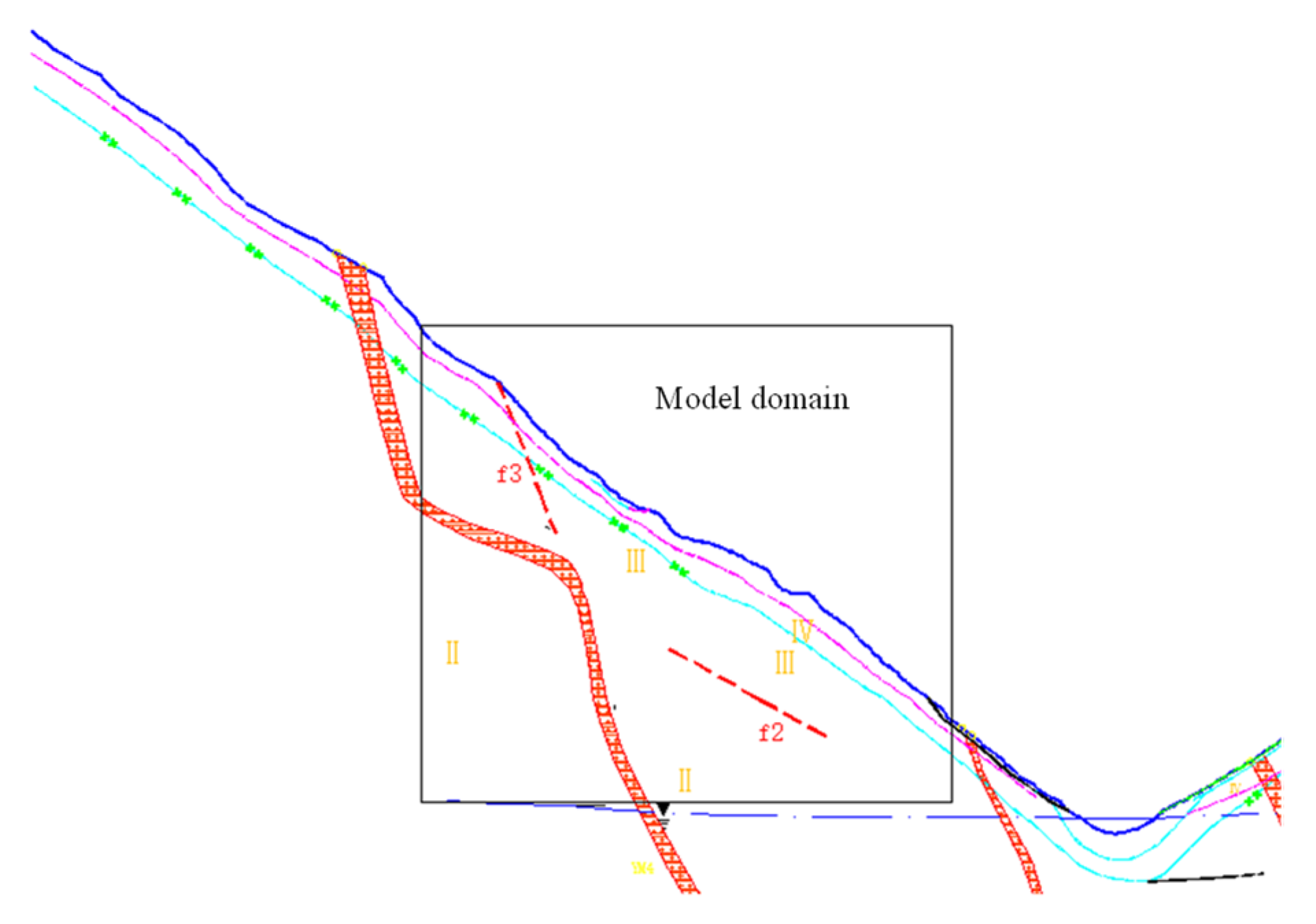
Figure 2.
Physical model diagram (cm). II: Class II rock mass. III: class III rock mass. IV: class IV rock mass.
Figure 2.
Physical model diagram (cm). II: Class II rock mass. III: class III rock mass. IV: class IV rock mass.
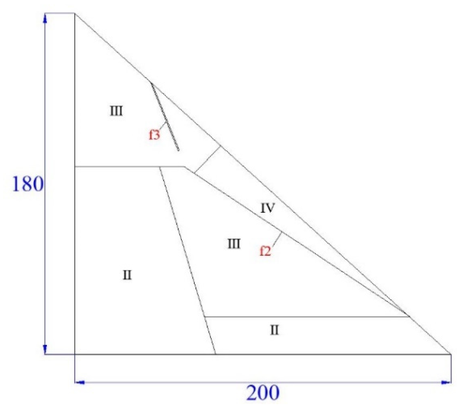
Figure 3.
The refrigeration and insulation equipment. (a) Large-scale test cold storage unit. (b) Incubator in the cold storage unit.
Figure 3.
The refrigeration and insulation equipment. (a) Large-scale test cold storage unit. (b) Incubator in the cold storage unit.
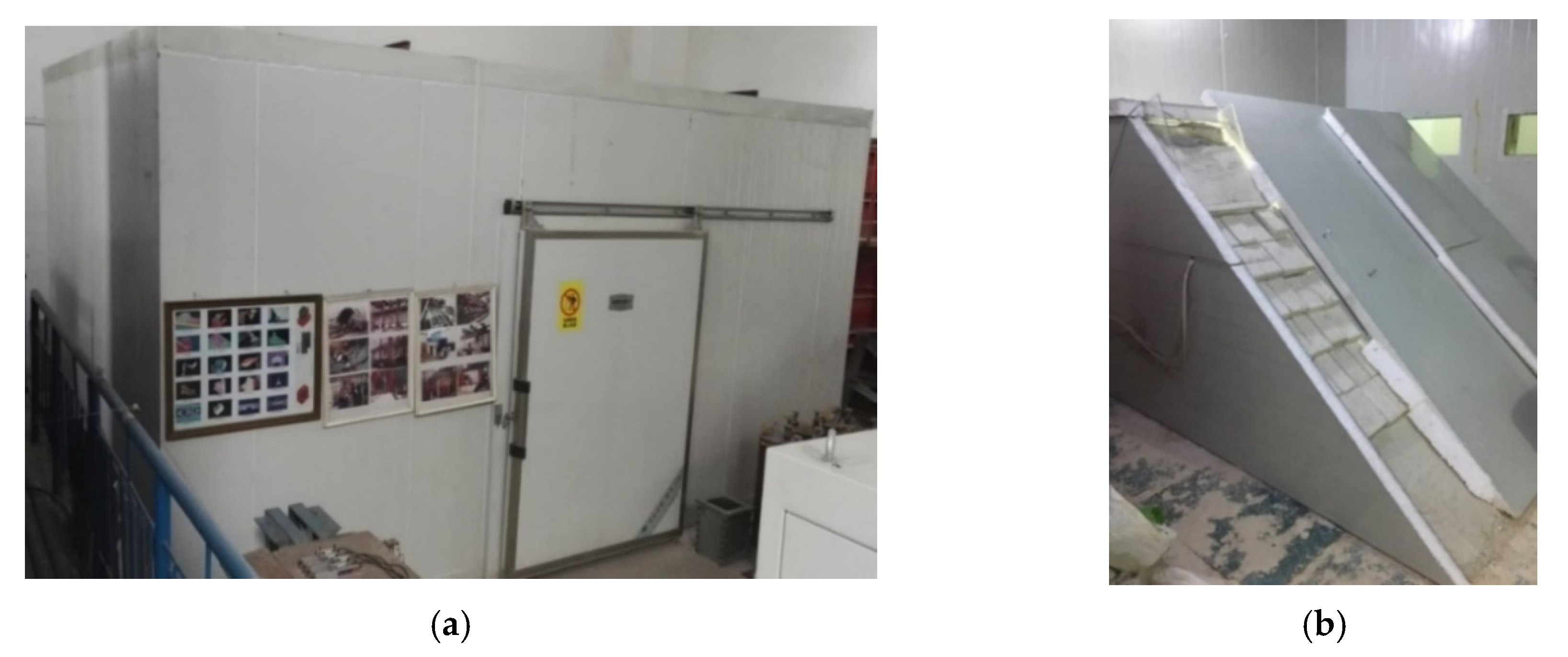
Figure 4.
The installation of the indoor model testing equipment. (a) Design drawing (cm). (b) Completed installation.
Figure 4.
The installation of the indoor model testing equipment. (a) Design drawing (cm). (b) Completed installation.

Figure 5.
The temperature change curves during the freeze–thaw processes: (a) cooling; (b) heating.

Figure 6.
The variation curves of the measured variables during the cooling process.
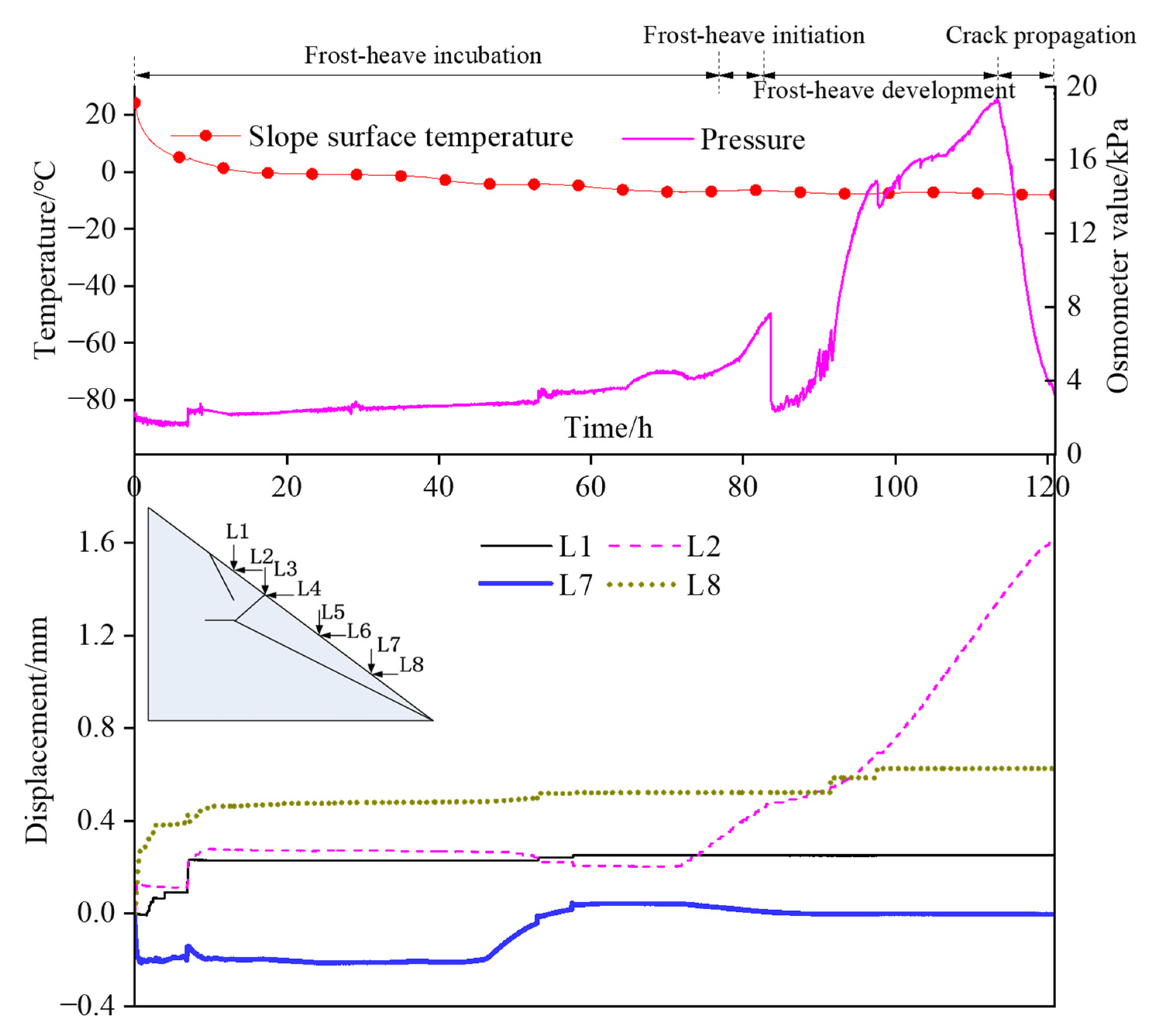
Figure 7.
The variation curves of the measured variables during the heating process.
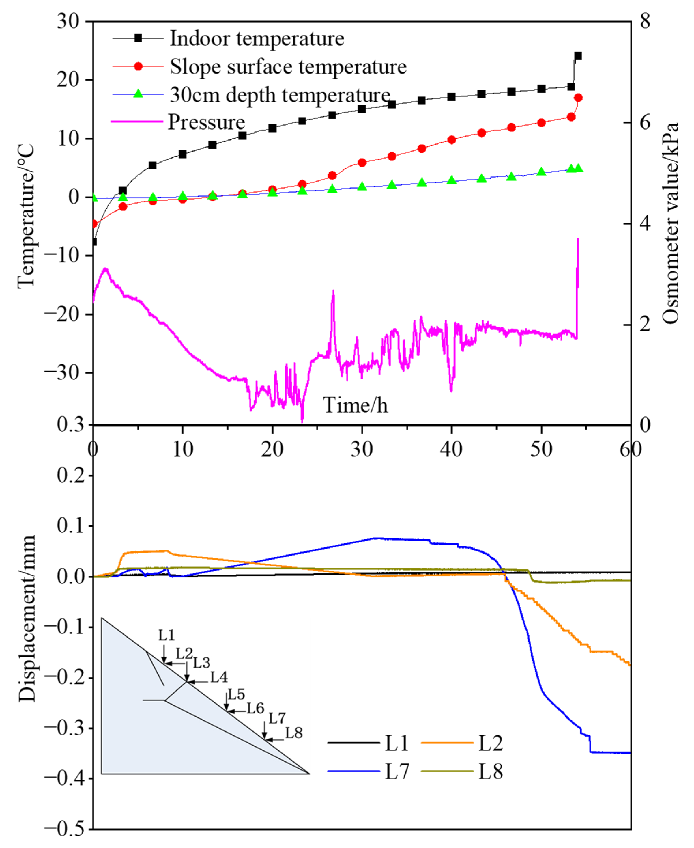
Figure 8.
Cracks caused by the freeze–thaw effect and their propagation paths.
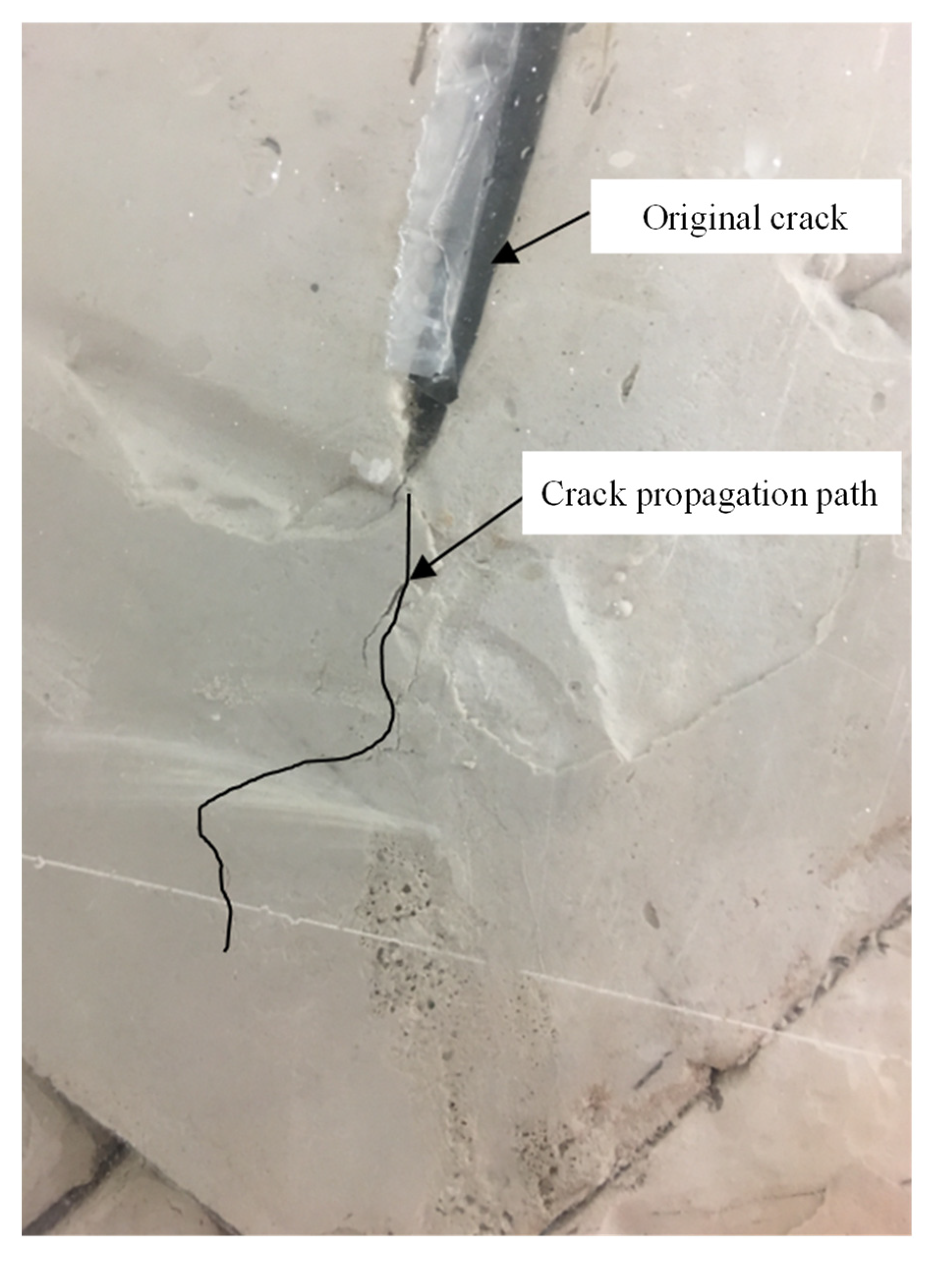
Figure 9.
The shape of the sliding slope caused by the freeze–thaw effect.
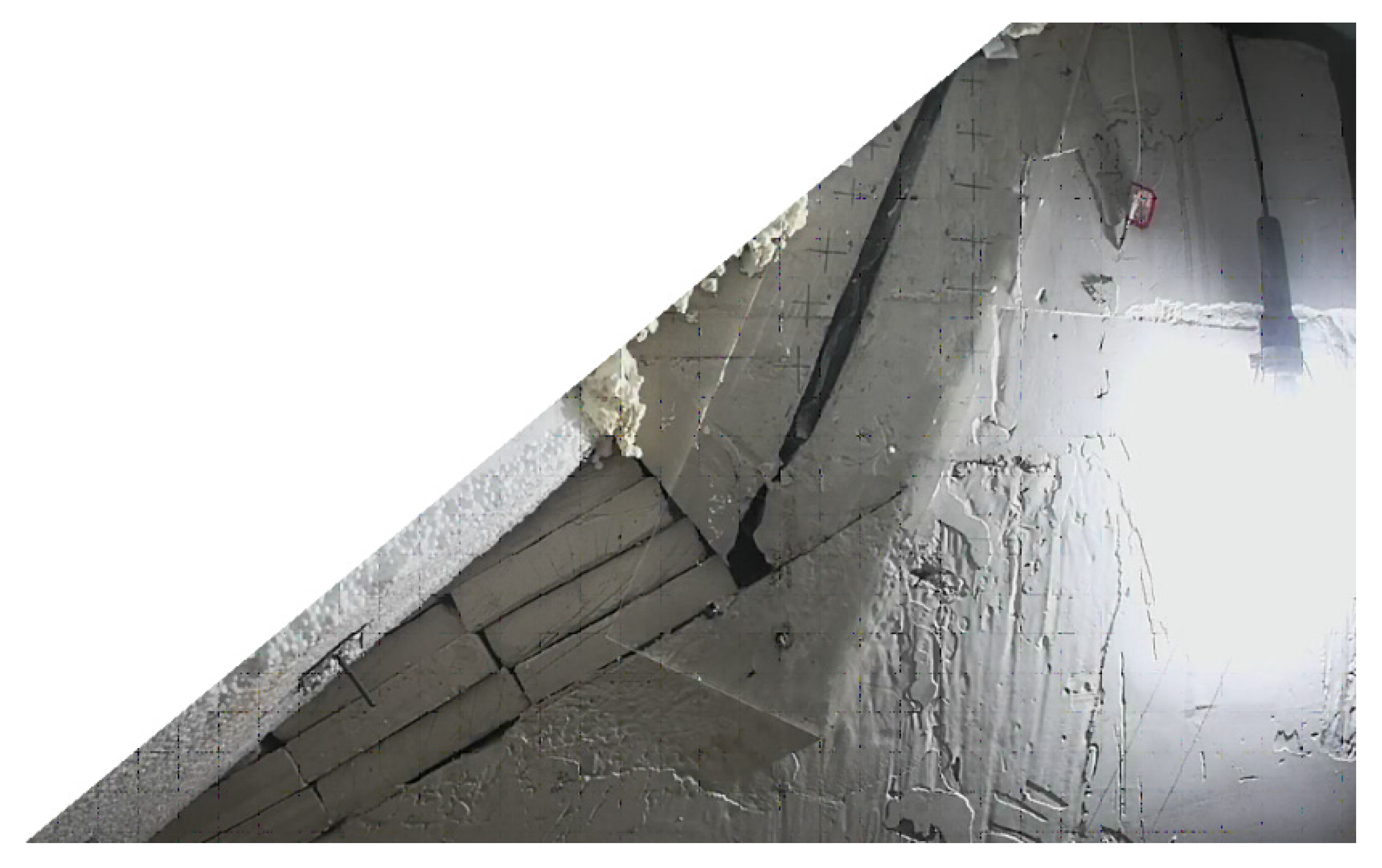
Figure 10.
The numerical model for frost-heave deterioration of rock slope. II: Class II rock mass; III: class III rock mass: IV: class IV rock mass.
Figure 10.
The numerical model for frost-heave deterioration of rock slope. II: Class II rock mass; III: class III rock mass: IV: class IV rock mass.

Figure 11.
Evolution diagrams of the minimum principal stress σ3 for the slope model: (a) 1 h; (b) 5 h; (c) 10 h; (d) 15 h; (e) 20 h.
Figure 11.
Evolution diagrams of the minimum principal stress σ3 for the slope model: (a) 1 h; (b) 5 h; (c) 10 h; (d) 15 h; (e) 20 h.
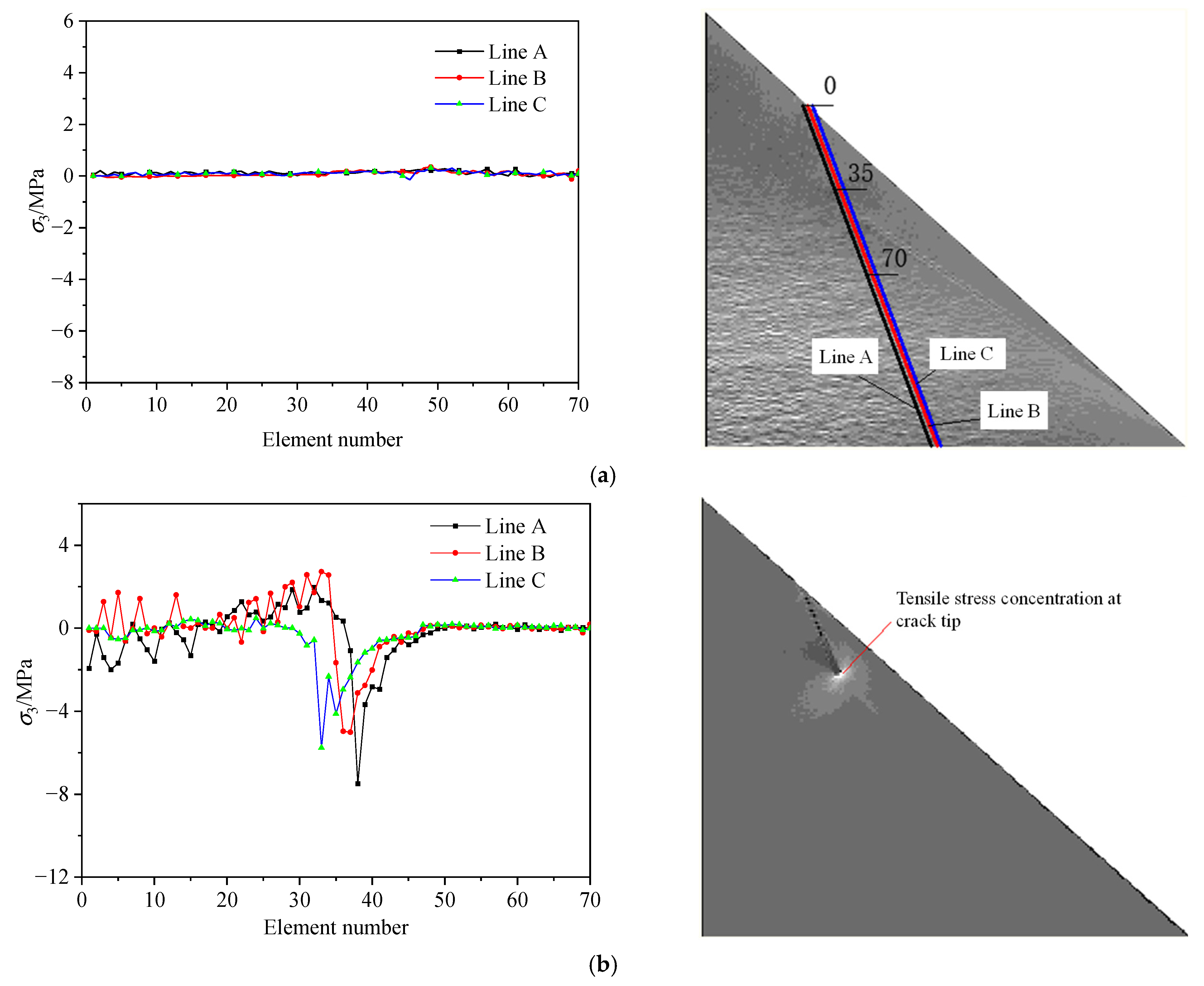
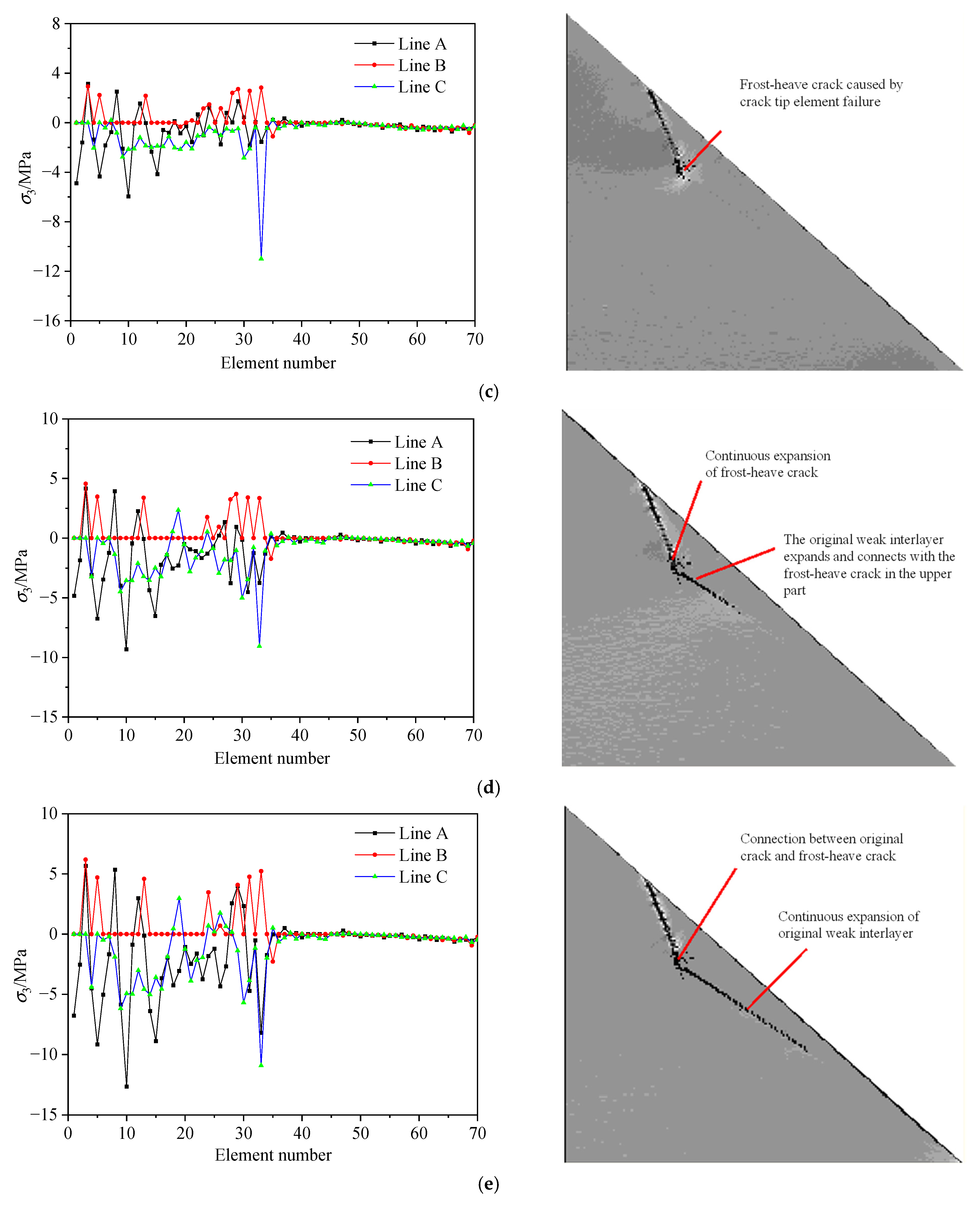
Figure 12.
Minimum principal stress distributions under different freezing rates: (a) freezing rate = 25%, σ3 = −6.18~4.51 MPa; (b) freezing rate = 50%, σ3 = −8.27~5.98 MPa; (c) freezing rate = 75%, σ3 = −10.9~9.06 MPa; (d) freezing rate = 100%, σ3 = −13.6~10.08 MPa.
Figure 12.
Minimum principal stress distributions under different freezing rates: (a) freezing rate = 25%, σ3 = −6.18~4.51 MPa; (b) freezing rate = 50%, σ3 = −8.27~5.98 MPa; (c) freezing rate = 75%, σ3 = −10.9~9.06 MPa; (d) freezing rate = 100%, σ3 = −13.6~10.08 MPa.
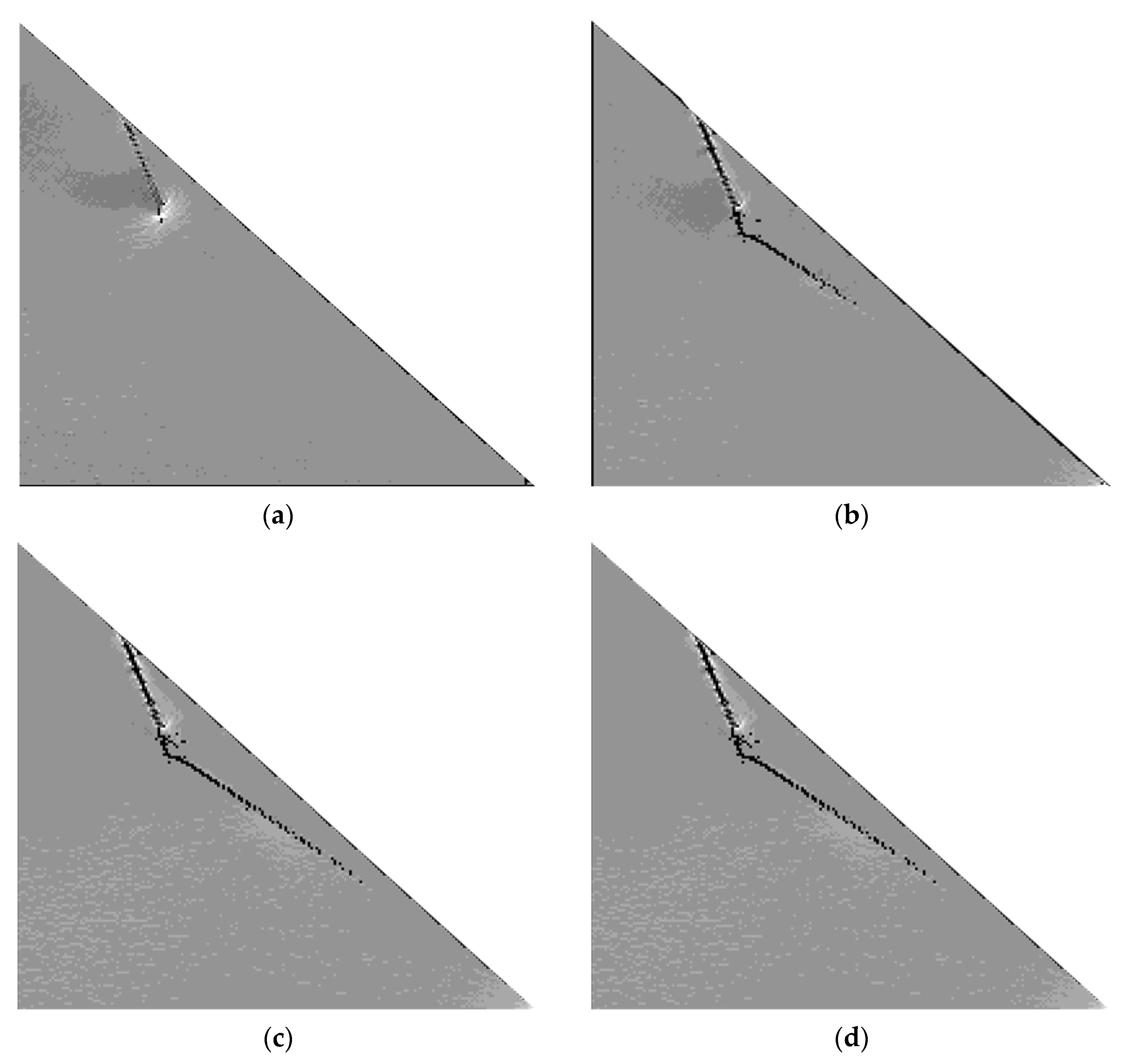
Figure 13.
The evolution of the minimum principal stress of typical elements under different ice contents.
Figure 13.
The evolution of the minimum principal stress of typical elements under different ice contents.

Table 1.
The physical and mechanical parameters of the physical model materials.
| Material Type | Unit Weight/kg/m3 | Elastic Modulus/GPa | Compressive Strength/MPa | Poisson’s Ratio | Cohesion/MPa |
|---|---|---|---|---|---|
| Indoor rock | 2710 | 38.83 | 112.28 | 0.35 | 11.1 |
| Quasi rock mass (Class III) | 2710 | 16.31 | 47.16 | 0.35 | 4.7 |
| Model material | 1656 | 0.13 | 0.49 | 0.25 | 0.04 |
Table 2.
The similarity constants of the materials.
| Similarity Constants | CL | Cγ | CE | CRc | Cμ | Cc |
|---|---|---|---|---|---|---|
| Actual value | 100 | 1.64 | 125.5 | 96.2 | 1.4 | 117.5 |
| Theoretical value | 100 | 1.64 | 164 | 164 | 1 | 164 |
Table 3.
The thermodynamic parameters of the numerical model.
| Materials | Thermal Capacity/(m3·°C) × 106 | Thermal Conductivity/(m·°C) | Coefficient of Thermal Expansion/°C × 10−5 | Ratio of Compression Strength to Tensile |
|---|---|---|---|---|
| Rock mass | 2.3 | 2.67 | 0.54 | 15 |
| Ice | 2.1 | 2.2 | −150 | 15 |
Table 4.
The physical and mechanical parameters of the numerical model.
| Unit Weight/kN/m3 | Elastic Modulus/GPa | Compressive Strength/MPa | Poisson’s Ratio | Internal Friction Angle/° | |
|---|---|---|---|---|---|
| Class II rock mass | 27.10 | 16.31 | 47.16 | 0.35 | 67.8 |
| Class III rock mass | 27.10 | 16.31 | 47.16 | 0.35 | 67.8 |
| Class IV rock mass | 27.00 | 12.30 | 39.13 | 0.38 | 65.7 |
| f2 | 24.00 | 1.5 | 6 | 0.4 | 30 |
| Ice | 9.17 | 0.6 | 6 | 0.35 | 20 |
Table 5.
The physical and mechanical parameters of the slope numerical model.
| Materials | Unit Weight kN/m3 | Elastic Modulus E/GPa | Compressive Strength σ/MPa | Poisson’s Ratio ν | Internal Friction Angle φ/° |
|---|---|---|---|---|---|
| Class II rock mass | 27.10 | 16.31 | 47.16 | 0.35 | 67.8 |
| Class III rock mass | 27.10 | 16.31 | 47.16 | 0.35 | 67.8 |
| Class IV rock mass | 27.00 | 12.30 | 39.13 | 0.38 | 65.7 |
| f2 | 24.00 | 1.5 | 6 | 0.4 | 30 |
Publisher’s Note: MDPI stays neutral with regard to jurisdictional claims in published maps and institutional affiliations. |
© 2022 by the authors. Licensee MDPI, Basel, Switzerland. This article is an open access article distributed under the terms and conditions of the Creative Commons Attribution (CC BY) license (https://creativecommons.org/licenses/by/4.0/).
Share and Cite
MDPI and ACS Style
Zhu, J.; Xu, D.; Wang, B.; Li, C. A Study on the Freeze–Thaw Damage and Deterioration Mechanism of Slope Rock Mass Based on Model Testing and Numerical Simulation. Appl. Sci. 2022, 12, 6545. https://doi.org/10.3390/app12136545
AMA Style
Zhu J, Xu D, Wang B, Li C. A Study on the Freeze–Thaw Damage and Deterioration Mechanism of Slope Rock Mass Based on Model Testing and Numerical Simulation. Applied Sciences. 2022; 12(13):6545. https://doi.org/10.3390/app12136545
Chicago/Turabian StyleZhu, Jiebing, Dongdong Xu, Bin Wang, and Cong Li. 2022. "A Study on the Freeze–Thaw Damage and Deterioration Mechanism of Slope Rock Mass Based on Model Testing and Numerical Simulation" Applied Sciences 12, no. 13: 6545. https://doi.org/10.3390/app12136545
Note that from the first issue of 2016, this journal uses article numbers instead of page numbers. See further details here.