The LOS/NLOS Classification Method Based on Deep Learning for the UWB Localization System in Coal Mines

Abstract

A localization system is one of the basic requirements for coal mines. Ultra-wideband (UWB), as a technology with broad application prospects, is considered to have great potential in the absence of satellite signals, especially in the underground mine environment, as it can provide rescue assistance. However, state-of-the-art UWB position systems in coal mines cannot efficiently differ the line-of-sight from all communication links, which results in deterioration of the localization accuracy. In this paper, we propose a LOS/NLOS classification method based on a deep learning algorithm. Specifically, we utilize the Generative Adversarial Networks (GAN) to generate diagnostic data for frame transmission under non-line-of-sight (NLOS) condition. Then, a Convolutional Neural Network (CNN) is adopted to identify the NLOS communication. Finally, the trilateral centroid positioning algorithm (TCPA) based on ranging data is used to verify the effect of our method for a localization system in coal mines. Field experiments show that our method can accurately differ the LOS/NLOS with the accuracy of 91.19%. The TCPA algorithm with our method can obtain 3.11% improvement compared with the scenario without using our method.

1. Introduction

In recent years, with the continuous development of wireless communication and wireless sensor network, wireless localization technology is widely used in disaster first aid, target tracking, vehicle navigation, pedestrian navigation, and other fields. Outdoor localization technology based on a global navigation satellite system has become viable. However in indoor and underground scenes without satellite signals, accurate localization has become a problem to be solved [1,2,3]. Ultra-wideband (UWB) has the advantages of high localization accuracy, high communication rate , strong multi-path resolution, and low power consumption. Thus, UWB has a good application prospect in the wireless localization field without satellite signals [4,5,6,7,8].

Facing the environment of an underground mine, in the existing UWB positioning systems, most of the channel impulse response (CIR) data of UWB are selected as the data for classifying NLOS [9,10,11]. However, because the length of the CIR data is too long, when the tag capacity is large, it may not be possible to obtain the full-length CIR data. In addition, in the actual use of UWB positioning system, the number of LOS data is usually larger than that of NLOS data. Even if all NLOS data is misidentified as LOS data, a high recognition rate can be achieved [12]. Thus, although NLOS data are scarce, they are more important than LOS data. Finally, after NLOS is identified, the distance value measured by UWB still contains other errors, and the positioning accuracy cannot be improved without eliminating them [13,14,15].

To address the aforementioned issues, we develop a LOS/NLOS classification method based on deep learning for the UWB localization system in coal mines. The problem of imbalanced classification and NLOS classification can be overcome in this study, and a person in a coal mine can be precisely located. However, it is worth mentioning that we merely introduced map limitations after the localization process to fix the results, while the actual situation needs to be considered much more than that. Nevertheless, the methods proposed in this paper, as a foundation, are constructive.

Our contributions in this paper are four-fold:

1

We propose a NLOS recognition method based on deep learning to distinguish whether a UWB signal transmission is blocked in coal mines. We use the diagnostic data in theDW1000 register as the data feature of deep learning, and analyze the classification performance of multilayer perceptrons and a convolutional neural network;

2

We propose a method for data enhancement based on generative adversarial networks (GAN) to solve the problem of class imbalance of data samples. We use this method to generate a new data set and compare the performance of the new data set with the original data set on the same classifier;

3

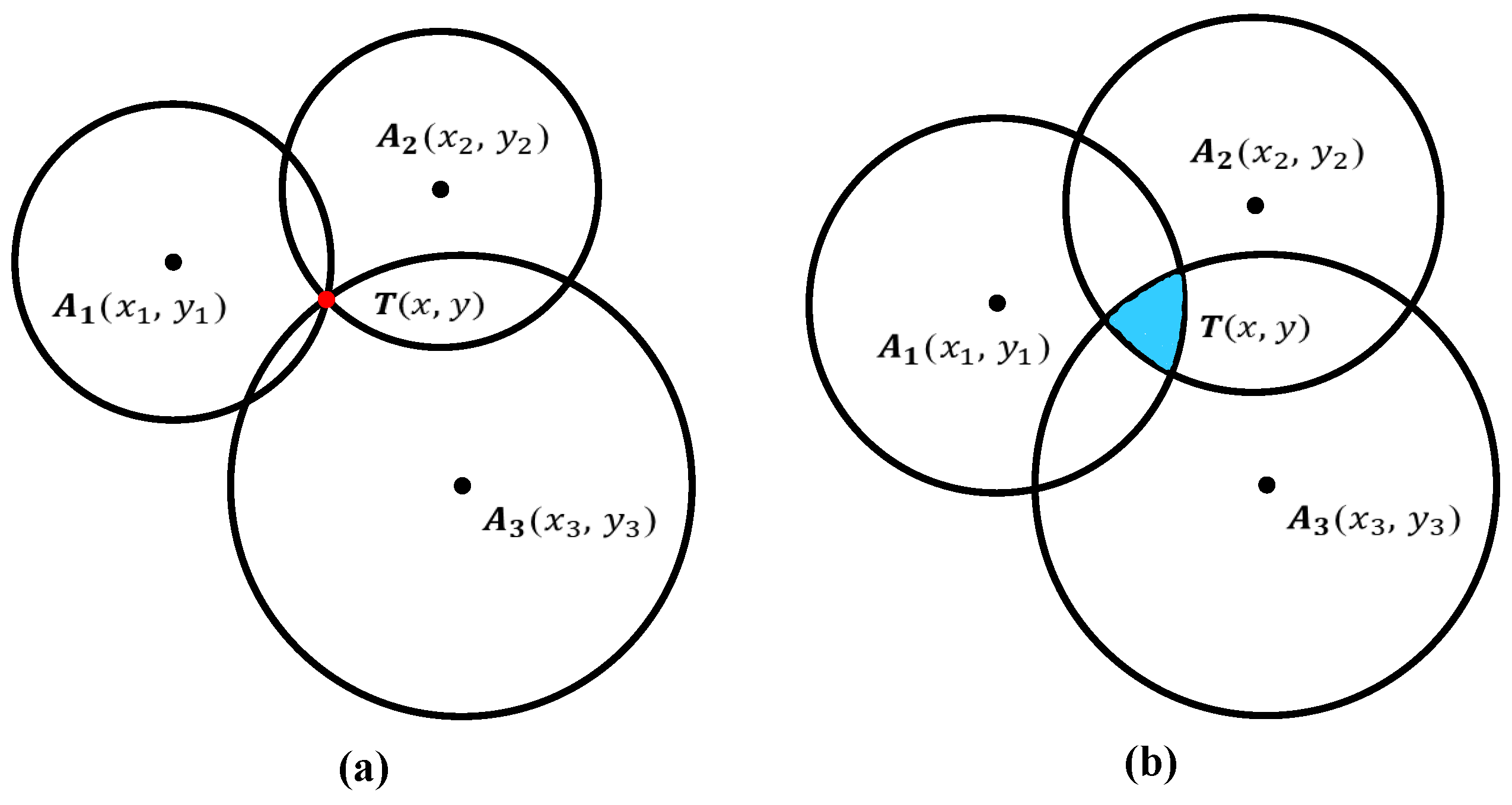
We propose a trilateral centroid positioning algorithm, and propose how to calculate the location result of the algorithm when a non-ideal situation occurs. Finally, we corrected the results with the map constraints;

4

We designed static and dynamic experiments to verify our system, and evaluated the proposed techniques through experiments and analysis.

The rest of this paper is structured as follows. Section 2 reviews the related works and presents the system architecture that we propose. Section 3 and Section 4 describe the mathematical principles of the method used in the system. Section 5 introduces our experimental system and analyzes and discusses the experimental results. Finally, we present our conclusions in Section 6.

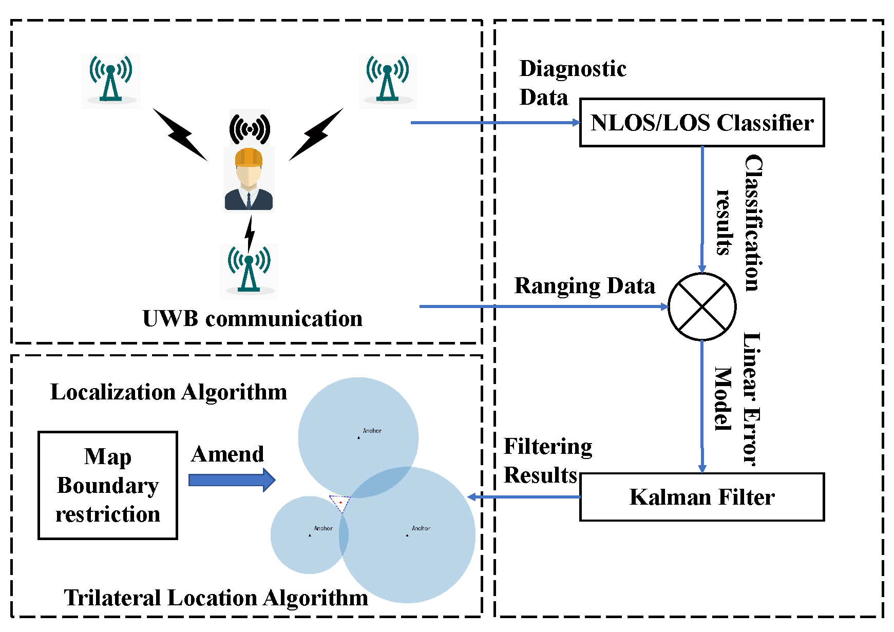
2. Related Work and Positioning System Structure

In order to solve the above problems, many people have begun to do research on a UWB positioning system. C Jiang et al. selected the CIR data as input of CNN-LSTM model to classify NLOS/LOS [16]. CL Sang et al. selected 12 features of the UWB signals as data features, and compared the data classification performance of the SVM, RF, and MLP models [17]. By et al. proposed to use a GAN and auto-encoder to enhance the training classification model and achieve better recognition performance [18]. Song Bo et al. proposed a fast imbalanced binary classification method based on moments (MIBC) to identify the NLOS signals [12]. K Kaemarungsi et al. adopted a fingerprint algorithm to do localization [19]. H Van Trees et al. proposed to utilize the prior information to improve the localization accuracy of the system [20]. A Poulose et al. used a deep long short-term memory network to extract more features from user distance information [21]. S Djosic et al. designed a hybrid algorithm based on fingerprint algorithm to identify NLOS in different environments [22].

After referring to the related work of others, we proposed our positioning system. Figure 1 shows the frame diagram of our positioning system.

As shown in Figure 1, our positioning system consists of three components: UWB communication, UWB data processing, and localization algorithm. When a coal mine worker enters the positioning area with a UWB tag, the tag will actively communicate with three nearby anchors. Each anchor calculates the distance value between the anchor and the tag based on the time-of-flight principle, and the register in the anchor device will record the frame transmission diagnostic data of the last data frame received during each communication. After completing each ranging, the anchor will transmit ranging data and frame transmission diagnostic data to the host computer. We trained a convolutional neural network that can utilize frame-transfer diagnostic data for NLOS/LOS classification. Then the linear model and Kalman filter are used to eliminate the errors in the ranging data. When the ranging data of the three anchors are processed through the above steps, the localization result is obtained by using the trilateral centroid localization algorithm. Finally, we correct our results with map constraints and display the results. We will describe the whole components in detail in the next two sections.

3. Nlos and Los Classification Based on Deep Learning Algorithm

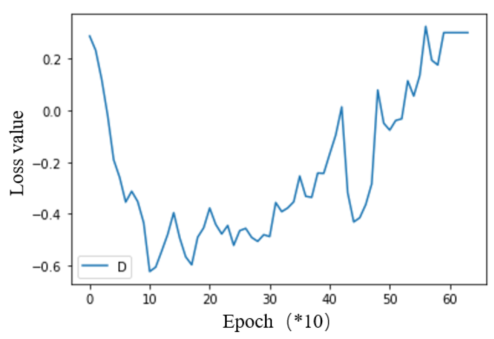
3.1. Data Augmentation by Generative Adversarial Networks

For the problem of class imbalance, we adopt the generative adversarial networks (GAN) for data augmentation. A typical theoretical GAN network structure is shown in Figure 2.

GAN consists of two main parts: generator and discriminator. The main function of the generator is to generate the sample data. The main function of the discriminator is to distinguish the receive sample data from the “spurious data” generated by the generator. The generator and the discriminator are trained at the same time, competing against each other. The loss function of GAN (cross entropy loss function) can be expressed as [23]:

$$\underset{G}{min}\underset{D}{max}V(D,G)={\mathbb{E}}_{x\sim p_{data}\left(x\right)}\left[{log}_{}D\left(x\right)\right]+{\mathbb{E}}_{x\sim p_z\left(z\right)}\left[{log}_{}(1-D(G\left(z\right)\left)\right)\right]$$

(1)

where $p_{data}\left(x\right)$ represents the distribution of real data and $p_z\left(z\right)$ represents the distribution of generated “spurious data”.

WGAN-GP network is a proposed variant based on the basic GAN network, which can solve the problem of unstable training of the original GAN network. The optimization function of WGAN-GP can be expressed as:

$$L=\underset{\tilde{x}\sim {\mathbb{P}}_g}{\mathbb{E}}\left[D\left(\tilde{x}\right)\right]-\underset{x\sim {\mathbb{P}}_r}{\mathbb{E}}\left[D\left(x\right)\right]+\lambda \underset{\widehat{x}\sim {\mathbb{P}}_{\widehat{x}}}{\mathbb{E}}\left[{({∥{\nabla }_{\widehat{x}}D\left(\widehat{x}\right)∥}_2-1)}^2\right]$$

(2)

where $\tilde{x}⟵G\left(z\right)$, $\widehat{x}⟵\epsilon x+(1-\tilde{x})$, $\epsilon \sim U[0,1]$, ${\mathbb{P}}_{·}$ represent the distribution of ·.

WGAN-GP adopts a new loss function, and the difference before the plus sign is called the Wasserstein distance. It is used to measure the distance or effort required to transform one distribution into another. The formula after the plus sign is called the Gradient penalty, which is a penalty term for the weight of D.

In GAN networks, the loss function for generators must be reduced, whereas the maximum loss function for discriminators must be optimized. By the max-min game, the generator and discriminator are trained alternately in a loop until the Nash equilibrium point is reached. At this time, after the Gaussian white noise is transformed by the generator, it can be used as a part of the data set for subsequent work to achieve the effect of data augmentation.

In order to solve the problem of class-imbalance, we train a GAN. We built the generator model and the discriminator model, shown in Figure 3. The coefficient of the penalty term $\lambda$ is taken as 0.3. During the training, the generator is responsible for generating “spurious data” by randomly generating latent data of shape [$batch\_size$, 4]. The discriminator receives both “spurious data” generated from generator and $batch\_size$ samples from the NLOS data.

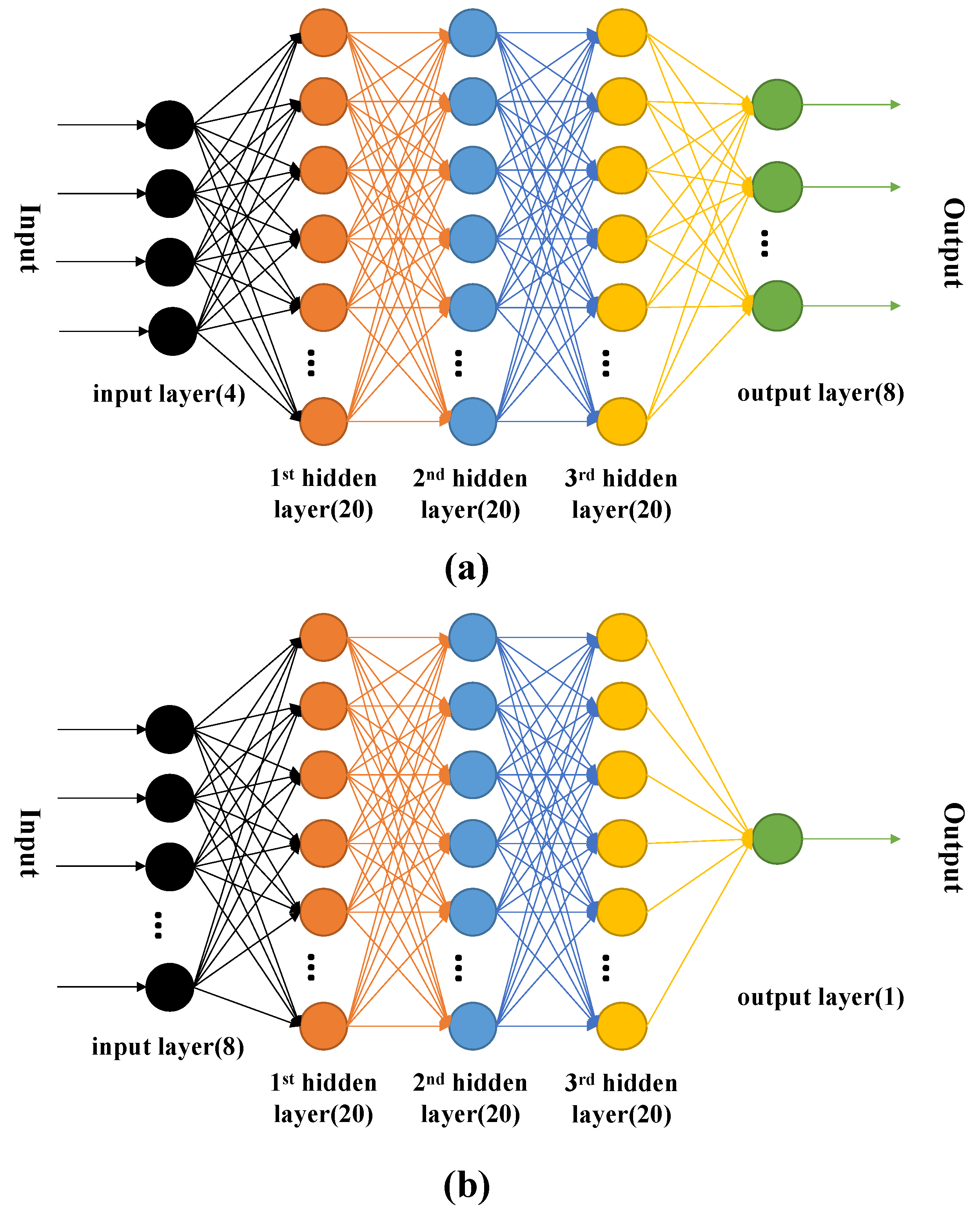
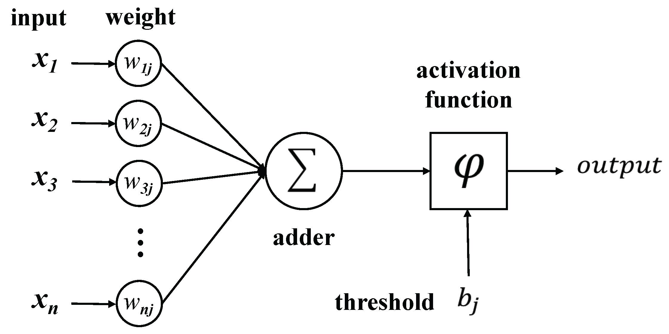
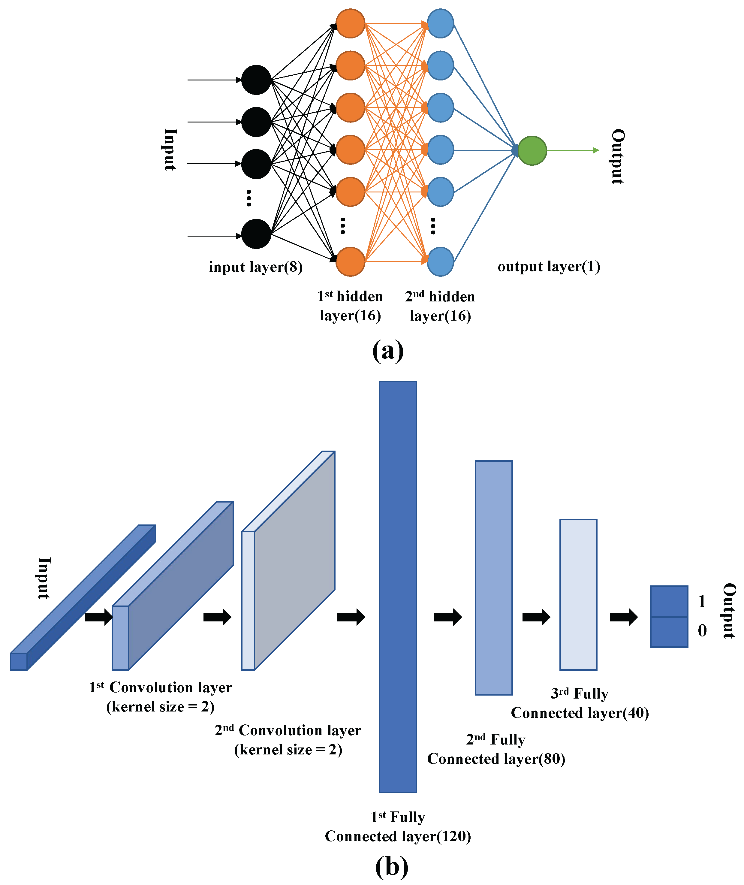
3.2. Multilayer Perceptrons for Classification Problems

Neural networks inspired by the human brain, also known as connectivity models, are not a recent technology. In 1958, Frank Rosenblatt proposed the first neural network with learning ability, called perceptron [24].

Artificial neurons are at the heart of all neural networks. Figure 4 shows a schematic of the basic structure of a neuron. It consists of two main parts: an adder that weights the sum of all inputs to the neuron, and a processing unit that produces an output according to a predefined function called the activation function. Each neuron has its own set of weights and thresholds (bias), which it learns through different learning algorithms.

When only one of these neurons exists, it’s called a perceptron. When there are many such layers, it is called a multilayer perceptron (MLP). Figure 5 shows a schematic of the MLP structure. MLP have one or more hidden layers. These hidden layers have different numbers of hidden neurons. Each neuron in the hidden layer has the same activation function.

MLP learn by supervised learning algorithms, that is, they provide the network with the ideal output of training data sets. At the output end, an error function or objective function $J\left(W\right)$ is defined so that the objective function will be minimal after the network has fully learned all the training data. A neuron can solve a linearly separable problem, while a learned MLP can solve a linearly indivisible problem.

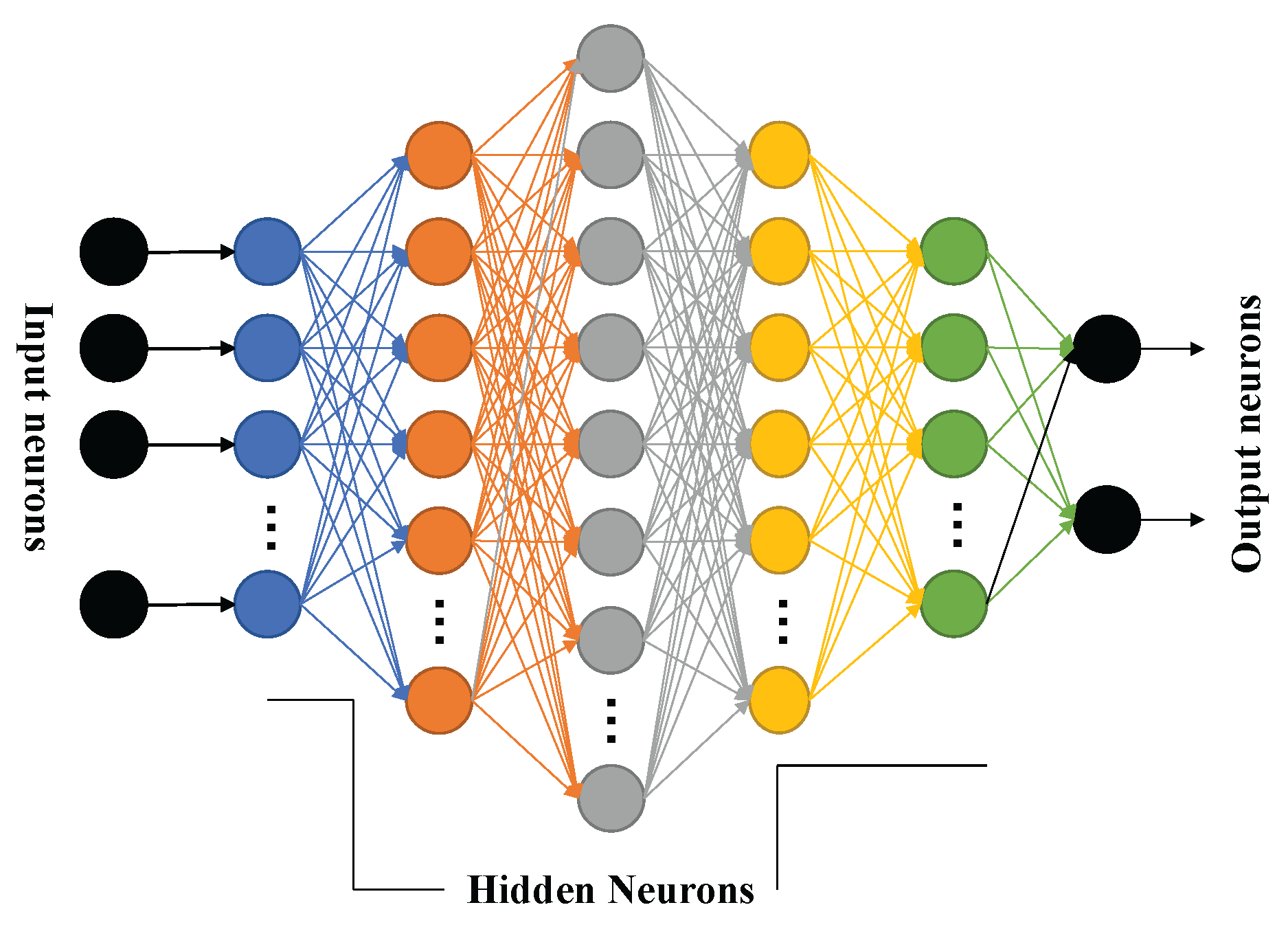
3.3. Convolutional Neural Networks for Classification Problems

The convolutional neural network (CNN) is a kind of feedforward neural network with deep structure and convolution computation. A CNN has the ability of representation learning, which can carry out shift-invariant classification of input information according to its hierarchical structure, and can carry out supervised and unsupervised learning. Figure 6 shows the basic structure of CNNs.

The convolutional layer is the most important layer in the whole neural network. The most core part of this layer is the convolutional kernel. The convolution process is designed to learn more complex features hidden in the data. After each convolution layer, a nonlinear layer (or activation layer) is usually applied immediately. The activation layer is generally followed by the pooling layer, which may substantially minimize the size of the matrix. Finally, there is a full connection layer before the output layer, which can integrate and normalize highly abstract features to learn these nonlinear combination features.

It is assumed that the CNN structure is composed of L hidden layers, where the input layer is denoted as 0-th layer, the output layer is $(L+1)$-st layer, and the output layer has K nodes, which represent K possible classes. The relation between the input of each layer and its output can be given as:

$$x^{(l+1)}=g\left(W^{\left(l\right)}{x}^{\left(l\right)}\right)$$

(3)

where $g(·)$ is the convolution layer, pooling layer, or full connection layer operation, $W^{\left(l\right)}$ and $x^{\left(l\right)}$ are the weights and the outputs of the l-th layer, respectively. The weights and inputs of hidden layers can be represented as$W_L=(W^{\left(1\right)},W^{\left(2\right)},\cdots ,W^{\left(L\right)})$ and $x_L=(x^{\left(1\right)},x^{\left(2\right)},\cdots ,x^{\left(L\right)})$, respectively. Therefore, the input and output relationship of CNN can be written as follows [25]:

$$x^{(L+1)}=\underset{W_L}{\underbrace{W^{\left(L\right)}{W}^{(L-1)}\cdots W^{\left(1\right)}}}{x}^{\left(0\right)}$$

(4)

Figure 7 shows the MLP and the CNN structures we designed, for the MLP model, we choose the $sigmoid$ function as the activation function of each neuron, and, for the CNN model, we choose the $relu$ function as the activation function of the hidden layer neurons.

4. Location Algorithm Based on Ranging

4.1. Composition of Ranging Errors

Since ranging needs to calculate the signal flight time, it is obvious that the propagation channel will reduce the ranging accuracy. The distance measurement error (DME) can be defined as:

$${\epsilon }_W\left(d\right)=\widehat{d_W}-d$$

(5)

where $\widehat{d_W}$ is the distance value calculated by the anchor based on DS-TWR, and d is the true distance between TAG and ANCHOR. The DME comes from multipath errors, errors in the process of measuring the real distance between the tag and the anchor, NLOS errors, and device antenna delay errors [26]. The random variable $\xi$ is used to model the occurrence of NLOS conditions, and the random variable takes a value of 1 when the NLOS condition occurs, otherwise the value is 0. Specifically, it can be expressed as:

$${\epsilon }_W\left(d\right)={\epsilon }_A+{\epsilon }_T+{\epsilon }_{M,W}\left(d\right)+\xi \ast {\epsilon }_{N,W}\left(d\right)$$

(6)

where ${\epsilon }_A$ is the error caused by the UWB device error, including antenna delay, crystal error, etc. Its value fluctuates to some extent. ${\epsilon }_T$ is the error caused by the operation or reading of the measuring instrument during the actual measurement of d, which approximately obeys the normal distribution, ${\epsilon }_{M,W}\left(d\right)$ is the error caused by multipath, and ${\epsilon }_{N,W}\left(d\right)$ is the error caused by NLOS condition. Figure 8 shows the NLOS condition and how the multipath error is generated.

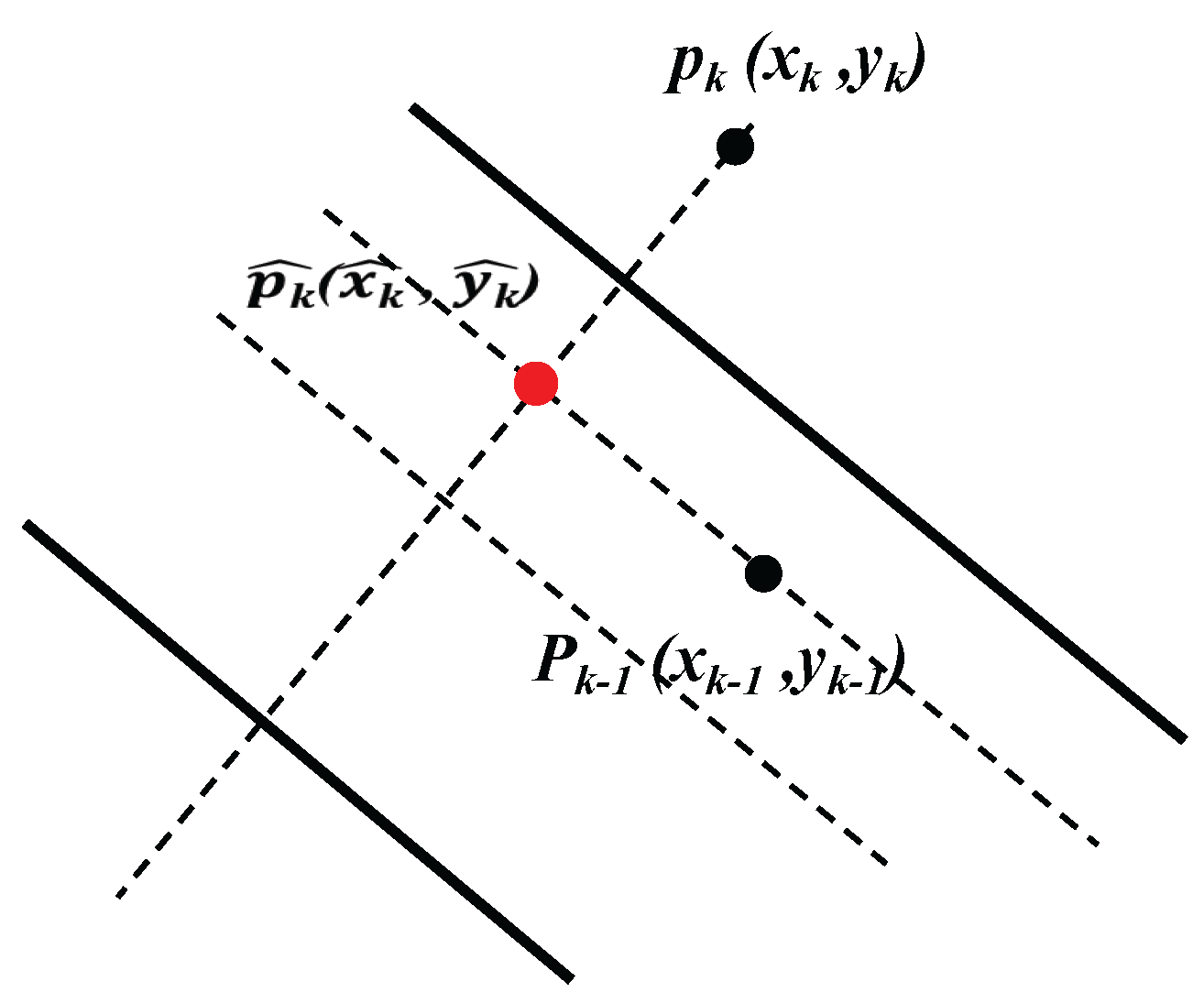
4.2. Linear Model and Kalman Filter

There are many ways to eliminate DME. The linear model equation used in this paper is as follows:

$$y=(1-\xi )(k_{los}·x+b_{los})+\xi (k_{nlos}·x+b_{nlos})$$

(7)

where y is the real distance between the tag and the anchor, x is the distance value calculated by the anchor based on TOF, $\xi$ is the state quantity of NLOS, and $k_{los}$, $b_{los}$, $k_{nlos}$, and $b_{nlos}$ are parameters corresponding to LOS and NLOS, respectively. The value of $\xi$ is based on the corresponding line-of-sight conditions during data collection, 1 for NLOS, and 0 for LOS.

Kalman filter is an algorithm that uses a series of data observed over time, which contains noise and other inaccuracies, to estimate unknown variables with more accuracy [27]. For ranging, the positioning system is a linear system. A discrete Kalman filter can be used to filter the ranging value. According to Equation (6), there are multiple errors in the DME. ${\epsilon }_A$ error includes clock drift error, and ${\epsilon }_T$ approximately obey normal distribution. Kalman filter can eliminate the errors caused by both and makes the data more stable.

We define the system state variable as $X_k\in R^n$, the system control input as $U_k$, and the system process excitation noise as $W_k$.Then the state equation of the system is:

$$X_k=A{X}_{k-1}+B{U}_k+W_k$$

(8)

The observed variable is $Z_k\in R^m$, and the observed noise is $V_k$. Thus, the measurement equation can be obtained as follows:

$$Z_k=H{X}_k+V_k$$

(9)

where H is the observation model matrix, which maps the real state space to the observation space. Assuming that $W_k$ and $V_k$ are mutually independent and normally distributed white noise, the process excitation noise covariance matrix is Q, and the observation noise covariance matrix is R, that is:

$$W_k\sim N(0,Q)$$

(10)

$$V_k\sim N(0,R)$$

(11)

The discrete Kalman filter includes the prediction process and update process. Prediction equations can be expressed as follows:

$${\widehat{X}}_k^{-}=A{\widehat{X}}_{k-1}+B{\widehat{U}}_{k-1}$$

(12)

$$P_k^{-}=A{P}_{k-1}{A}^T+Q$$

(13)

Update equations are expressed as follows:

$$K_k=P_k^{-}{H}^T{(H{P}_k^{-}{H}^T+R)}^{-1}$$

(14)

$${\widehat{X}}_{k-1}={\widehat{X}}_k^{-}+K_k(Z_k-H{\widehat{X}}_k^{-})$$

(15)

$$P_k=(I-K_{k}H)P_k^{-}$$

(16)

where $K_k$, ${\widehat{X}}_k$, $P_k$, I is the Kalman gain matrix, the optimum filter value, the filter deviation matrix, and the unit matrix, respectively.

The prediction process mainly uses the prediction equation to establish a priori estimation of the current state, and predicts the current state variable and the value of the error covariance estimate forward in time, so as to construct a priori estimate for the next time state; the more trust process is responsible for feedback, and using the prediction equation establishes an improved posterior estimate of the current state based on a priori estimates of the prediction process and current measured variables.

4.3. Trilateral Centroid Positioning Algorithm

The positioning method of the UWB positioning system can use the trilateral centroid positioning algorithm (TCPA). Figure 9 shows the schematic diagram of the original trilateral centroid positioning algorithm.

In the two-dimensional plane coordinate system, it is known that the coordinates of the three anchors are $A(x_1,y_1),A(x_2,y_2),A(x_3,y_3)$, and the coordinates of the tag are $T(x,y)$. The distances between the tag and the three anchors are $r_1,r_2$ and $r_3$, respectively. Taking the three anchor coordinates as the center and the corresponding r as the radius, three circles can be formed. They have the following relationship:

$$\left\{\begin{array}{c}{(x-x_1)}^2+{(y-y_1)}^2=r_1^2\hfill \\ {(x-x_2)}^2+{(y-y_2)}^2=r_2^2\hfill \\ {(x-x_3)}^2+{(y-y_3)}^2=r_3^2\hfill \end{array}\right.$$

(17)

Ideally, as shown in the Figure 9a, three circles intersect at a point. However, when there are errors in $r_1,r_2$, and $r_3$ as shown in the Figure 9b, they will not intersect at one point. Tag is in the blue area, where the optimal position needs to be found.

The principle of TCPA is to use the centroid of a triangle determined by pairs of circles as the location result. There are five types of relations between two circles: intersection, inner tangent, outer tangent, inner separation, and the outer separation. Figure 10 shows the schematic diagram of the two positioning processes including these five relations.

When two circles are tangent, the tangent point($P_t$ in the Figure 10a,b) is directly used as the vertex determined by the two circles.

When two circles are separated, the vertex determined by the two circles is the midpoint at which they are closest to each other, just as point $P_s$ in Figure 10a,b.

When the two circles intersect, the vertex determined by the two circles is the intersection point at which the sum of the sides of the triangle with the other vertices determined or to be determined is the smallest, just as the point $P_{i1}$ in Figure 10a and the point $P_{i2}$ in Figure 10b.

After determining the vertex of the triangle, we calculate the centroid of the triangle, which is the positioning result of TCPA. When we calculate the centroid coordinates of a triangle determined by the TCPA, it may fall outside the boundary of the map if we display it directly. So it needs to be corrected when it falls outside the boundaries of the map. Figure 11 shows a schematic diagram of the corrected positioning results.

We oass point $P_k$ to take a normal line of the map boundary and extend it. The corrected positioning result should fall on the normal line; pass point $P_{k-1}$ to take a parallel line (or curve) of the map boundary, then it will intersect the normal at point ${\widehat{p}}_k$. Point ${\widehat{p}}_k$ must fall within the map boundaries, therefore taking it as the corrected result.

5. Experiment, Results and Discussion

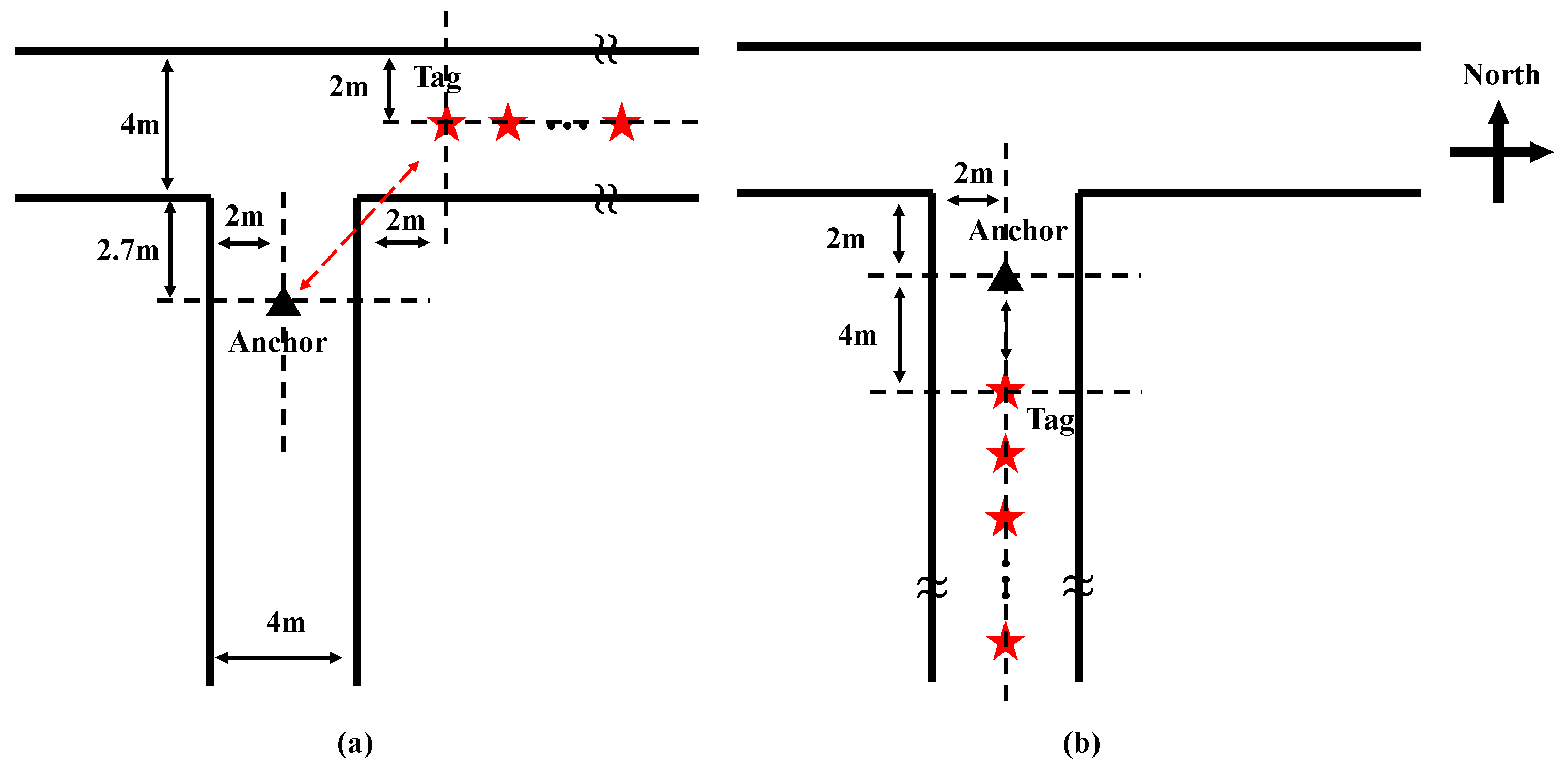
5.1. Experiment Set Up and Data Collection

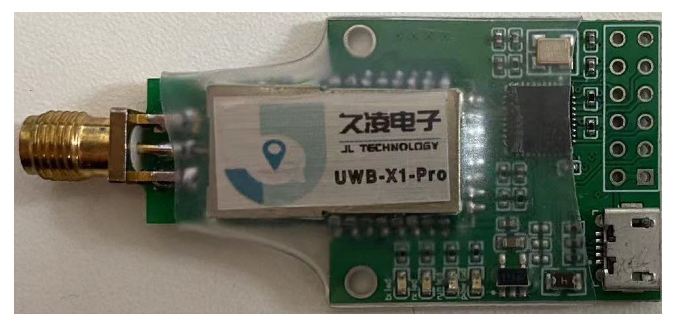
5.1.1. Hardware Platform

As shown in the Figure 12, we use the device based on DW1000 [28] as the tag and the anchor. Ranging using a TOF based ranging method.

5.1.2. Data for Training Network Model

We use the diagnostic data as the input data for our classifier. So both the MLP model and the CNN model we established have eight input neurons. As shown in

Table 1. Symbols of the frame transmit data we used to read from the registers.

Serial Number	Symbols	Meaning
1	firstPathAmp1	the magnitude of the accumulator tap at the index 3 beyond the integer portion of the rising edge FP_INDEX reported in Register
2	firstPathAmp2	the magnitude of the accumulator tap at the index 2 beyond the integer portion of the rising edge FP_INDEX reported in Register
3	firstPathAmp3	the magnitude of the accumulator tap at the index 1 beyond the integer portion of the rising edge FP_INDEX reported in Register
4	stdNoise	the standard deviation of the noise level seen during the LDE algorithm’s analysis of the accumulator data.
5	maxGrowthCIR	a growth factor for the accumulator which is related to the receive signal power.
6	firstPathIdex	the position within the accumulator that the LDE algorithm has determined to be the first path.
7	rxPreamCount	the number of symbols of preamble accumulated.
8	C	the Channel Impulse Response Power value reported in the CIR_PWR field of Register file

, eight symbols of the transmitting data are involved in our diagnostic data.

According to the DW1000 Software API Guide and the DW1000 user manual, in the above diagnostic data, $stdNoise$ reported in the register file may be used to give a measure of the noise associated with this and the received frame’s timestamp measurement. firstPathAmp1, firstPathAmp2, firstPathAmp3 are 16-bit unsigned values that are part of reporting the magnitude of the leading edge signal seen in the accumulator data memory during the LDE algorithm’s analysis. In addition to stdNoise, other data types will be used to calculate the first path power level and the receive power level. High noise may mean that the real first path is irretrievably buried in the noise. Comparing the noise with the First Path Amplitude can give additional indication as to the quality of the first path measurement. So those features can be used in assessing the quality of the received signal. In order to obtain the LOS sample data and the NLOS sample data with these eight characteristics, we designed an experimental system to collect the LOS sample data and the NLOS sample data, respectively. Figure 13 shows a top view of our experimental scenario.

We marked the location of the tag, before the data is collected. For the collection of NLOS data, we moved 1 m to the east of the map each time, and collected a group of several NLOS samples at each location. A total of 11 moves can collect 12 sets of data. For the collection of LOS data, we move 2 m to the south of the map each time, and collect a set of LOS sample data of a certain number at each position, moving a total of 53 times, that is, 54 sets of data can be collected. Each sample data includes the ranging values and eight features described in the previous paragraph.

Table 2. The amount of sample data needed to train the model network.

NLOS/LOS	Number of Set	Total
NLOS	12	1812
LOS	54	6967
total	-	8779

shows the number of sample data collected by out experiments.

5.1.3. Data for Testing Position System

To test our designed localization system, we designed static and dynamic experiments to examine our system, respectively. Figure 14 shows the concept diagrams for our static and dynamic experiments.

For the static experiments, we fixed the three anchors in the positions shown in Figure 14a, The tag is placed in one of the three positions (red position, blue position, green position) at a time. The bidirectional arrows in the same color as the tag indicate the anchor ranging from the tag (dotted line indicates the NLOS, solid line indicates the LOS). When the tag is in each position, we collect the data transmitted by the three anchors. Each sampling data includes ranging value and eight features, and the laptop records the sample data from each anchor separately.

As shown in Figure 14b, for the dynamic experiment, we have the same setup as in the static experiment, where a person carries a tag from the red five-pointed star position as far as possible along the path of the dotted black arrow at a uniform speed until the green pentagram position ends. During the movement process, each anchor transmits the sampling data containing the ranging value and eight features of each ranging to the host computer.

Table 3. The amount of data collected by the experiment to test our designed positioning system. The data is obtained by one tag and three anchors, each performing a ranging as a group.

Static/Dynamic Experiment	Position	Amount of Sample Data (Group)
	red	70
Static experiment	blue	68
	green	68
Dynamic experiment	-	104

shows the amount of the data we collected from the static and the dynamic experiments.

5.2. Experimental Results and Discussion

5.2.1. Network Model Training Results and Discussion

The NLOS data and the LOS data are 1812 and 6967, respectively. There is five times of discriminator training in one training, and one training of the generator, with a total of 1000 times of training. According to the theory of GAN, we want to maximize the loss function of the discriminator as much as possible. The loss function of the discriminator is shown in Figure 15. It can be seen that the loss function of the discriminator gradually increased and stabilized near the maximum value.

After the GAN is trained, we put 2000 random Gaussian noise data into the generator to generate 2000 samples. We copied the original dataset and added those 2000 samples to form a new data set. Now our original data set includes 6967 LOS data and 1812 NLOS data, and the new data set includes 6967 LOS data and 3812 NLOS data. The two data sets are divided into the training set and the test set according to the ratio of 7:3. We use these training sets to train the MLP model and CNN model, and test our model with the same test set.

After the network model is trained, on the same test set, the performance of MLP model and CNN model trained by the training set of the original data set is 88.0790% and 90.8125%, respectively. The performance of the MLP model and CNN model trained by the training set of the new data set is 89.1420% and 91.1921% respectively. We further evaluate the performance of our model using the $classification\_report\left(\right)$ function from the machine learning $scikit$-$learn$ library. The performance of our trained MLP models and the performance of our trained CNN models are shown in the

Table 4. Performance of our trained MLP models.

Using the Data Generated by the Generator		Precision	Recall	f1-Score	Support
	LOS	0.89	0.96	0.93	2092
NO	NLOS	0.80	0.56	0.66	542
	accuracy			0.88	2634
	LOS	0.91	0.95	0.93	2092
YES	NLOS	0.78	0.65	0.71	542
	accuracy			0.89	2634

and

Table 5. Performance of our trained CNN models.

Using the Data Generated by the Generator		Precision	Recall	f1-Score	Support
	LOS	0.93	0.96	0.94	2092
NO	NLOS	0.82	0.72	0.76	542
	accuracy			0.91	2634
	LOS	0.94	0.95	0.94	2092
YES	NLOS	0.79	0.77	0.78	542
	accuracy			0.91	2634

, separately.

As can be seen from Table 4 and Table 5, the precision of the MLP model trained by the training set of the original and new data sets for the NLOS class is 0.80 and 0.78, the recall is 0.56 and 0.65, and the f1-score is 0.66 and 0.71, respectively. The accuracy of all samples are 0.88 and 0.89, respectively. The precision of the CNN model trained by the training set of the original data set and the new data set for the NLOS class is 0.82 and 0.79, the recall is 0.72 and 0.77, and the f1-score is 0.76 and 0.78, respectively. The accuracy of all samples is 0.91. After the GAN model is used to enhance the data, the recall of NLOS data in MLP model and CNN model is increased by 9% and 5% respectively, and the f1-score is increased by 5% and 2% respectively. This means that GAN data enhancement can improve the performance of the network model. In horizontal comparison, after the GAN model is used to enhance the data, the CNN model performs better than the MLP model in terms of the recall and f1-score of both LOS and NLOS class.

In conclusion, data enhancement by GAN can improve the performance of the network model. By comparing the performance of MLP model and CNN model, it can be seen that the CNN model has better performance.

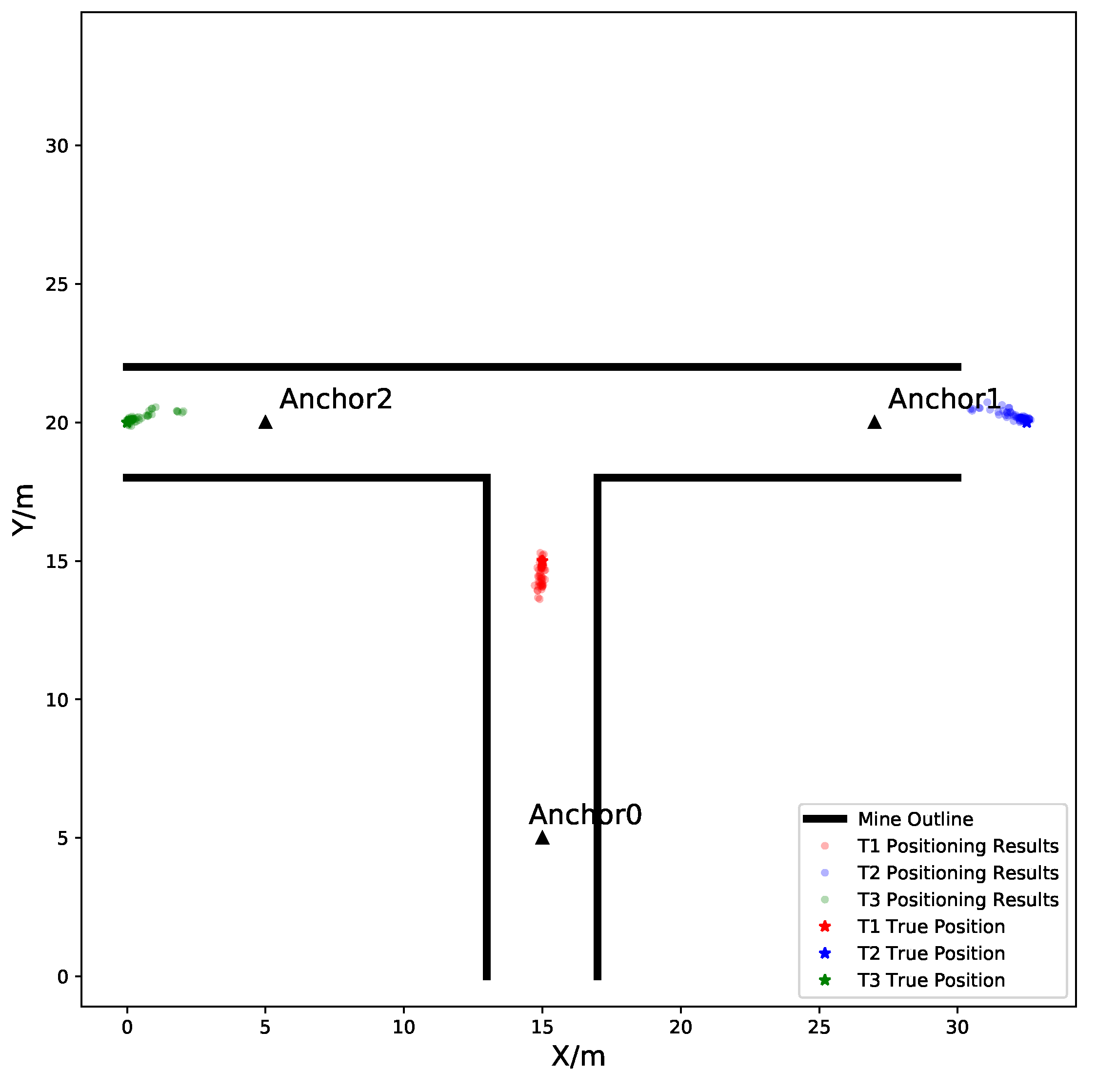
5.2.2. Localization System Test Results and Discussion

In the static experiment, we collected about 70 data sets at three positions, respectively. Figure 16 and Figure 17 show the results and localization errors of this static experiment. Since Kalman filter parameter initialization requires a certain number of filtering times, the localization results and the calculation results of removing the first five groups of data by localization error are shown in Figure 16 and Figure 17.

As can be seen from Figure 16, most of the localization results are beside the corresponding real positions. For Figure 17, we define the error as the distance between the real position and the position calculated by the localization system. For T1, T2, and T3, the average errors of our system localization are 0.47 m, 0.54 m, and 0.42 m, respectively. The reason why the error reaches 1 M or even 2 m is that NLOS is wrongly identified as LOS. The error in ranging cannot be eliminated in the linear model, so the error will be transferred to the positioning process in the subsequent process, resulting in a large location error. As T2 and T3 are located on one side of all anchors, the distance errors cannot cancel each other, and their location errors are larger than T1.

Figure 18 shows the results of the dynamic experiment. Since the real position of the tag at each moment could not be determined during the dynamic experiment, we could not calculate the error and could only compare the real track of tag with the track formed by the location result of our location system. As can be seen from Figure 18, the location at the first few moments has a large error, which is mainly due to the slow initialization of the Kalman filter parameters. When the parameters of the Kalman filter are gradually stabilized, the localization accuracy of the system begins to improve, and the movement track of the tag calculated by the system is almost consistent with that of the real tag. The reason for the large deviation of the location track lies in the error of the NLOS/LOS classification of the tag and one of the three anchors, which leads to the location deviation.

According to the results of static and dynamic experiments, the accuracy of our localization system can reach decimeter level in complex tunnel environment. It can not only get the position of motionless personnel, but also track and locate the moving personnel in real time. When the line-of-sight condition is occasionally misidentified, the positioning result will have a large error. However this error is rare and permitted in the coal mine environment.

6. Conclusions

In this paper, we develop a personnel localization system for coal mines. On the one hand, we propose to use frame transmission diagnostic data for line-of-sight classification. From the classification results, CNN model has high classification accuracy for our data and can be used as our NLOS/LOS classifier. Compared with MLP, it has a higher f1-score, higher classification accuracy, and better performance for NLOS. On the other hand, we design a complete localization system, including the calculations used from data acquisition to the calculation of location results. From the results of static and dynamic experiments, it can be seen that our system has good localization performance for static or moving tags. For static tag, localization accuracy of half a meter can be achieved; For a moving tag, we can track the movement of the tag well. However, in different tunnel environments, different ranging environments will lead to different signals, so the robustness for different environments is low. In out future work, we will focus on the concurrency problem when the tag capacity is large.

References

1. Choliz, J.; Eguizabal, M.; Hernandezsolana, A.; Valdovinos, A. Comparison of Algorithms for UWB Indoor Location and Tracking Systems. In Proceedings of the 2011 IEEE 73rd Vehicular Technology Conference (VTC Spring), Budapest, Hungary, 15–18 May 2011. [Google Scholar]
2. Cheng, L.; Zhao, A.; Wang, K.; Li, H.; Chang, R. Activity Recognition and Localization based on UWB Indoor Positioning System and Machine Learning. In Proceedings of the 2020 11th IEEE Annual Information Technology, Electronics and Mobile Communication Conference (IEMCON), Vancouver, BC, Canada, 4–7 November 2020. [Google Scholar]
3. Li, B.; Zhao, K.; Saydam, S.; Rizos, C.; Wang, J.; Wang, Q. Third Generation Positioning System for Underground Mine Environments: An Update on Progress; Far East Journal of Electronics and Communications (FJEC): Prayagraj, India, 2018. [Google Scholar]
4. Aca, B.; Pf, B.; Pmt, B. UWB-based sensor networks for localization in mining environments. Ad Hoc Netw. 2009, 7, 987–1000. [Google Scholar]
5. Capraro, F.; Segura, M.; Sisterna, C. Human Real Time Localization System in Underground Mines using UWB. IEEE Lat. Am. Trans. 2020, 18, 392–399. [Google Scholar] [CrossRef]
6. Zheng, X.; Wang, B.; Zhao, J. High-precision positioning of mine personnel based on wireless pulse technology. PLoS ONE 2019, 14, e0220471. [Google Scholar] [CrossRef] [PubMed] [Green Version]
7. Bao, J.; Wang, H.; Research on Key Technologies of High-Precision Location Based Service System for Intelligent Mines. ResearchGate.PrePrint. Version 1. Posted 17 December 2020. Available online: https://www.sciencegate.app/app/document/download#10.21203/rs.3.rs-127354/v1 (accessed on 29 May 2022).
8. Ming, L. A Novel Ultra-Wideband Hybrid Localization Scheme in Coal Mine. J. Commun. 2015, 10, 889–895. [Google Scholar]
9. Yoon, J.; Kim, H.; Seo, D.; Nam, H. Performance Comparison of NLOS Detection Methods in UWB. In Proceedings of the 2021 International Conference on Information and Communication Technology Convergence (ICTC), Jeju Island, Korea, 19–21 October 2021; pp. 1486–1489. [Google Scholar] [CrossRef]
10. Liu, Q.; Yin, Z.; Zhao, Y.; Wu, Z.; Wu, M. UWB LOS/NLOS identification in multiple indoor environments using deep learning methods. Phys. Commun. 2022, 52, 101695. [Google Scholar] [CrossRef]
11. Altstidl, T.; Kram, S.; Herrmann, O.; Stahlke, M.; Feigl, T.; Mutschler, C. Accuracy-Aware Compression of Channel Impulse Responses using Deep Learning. In Proceedings of the 2021 International Conference on Indoor Positioning and Indoor Navigation (IPIN), Lloret de Mar, Spain, 29 November–2 December 2021; pp. 1–8. [Google Scholar] [CrossRef]
12. Song, B.; Li, S.L.; Tan, M.; Ren, Q.H. A fast imbalanced binary classification approach to NLOS identification in UWB positioning. Math. Probl. Eng. 2018, 2018, 1580147. [Google Scholar] [CrossRef]
13. Fan, R.; Du, X. NLOS Error Mitigation Using Weighted Least Squares and Kalman Filter in UWB Positioning. arXiv 2022, arXiv:2205.05939. [Google Scholar]
14. Liu, R.; Yuen, C.; Do, T.N.; Jiao, D.; Liu, X.; Tan, U.X. Cooperative Relative Positioning of Mobile Users by Fusing IMU Inertial and UWB Ranging Information. In Proceedings of the 2017 IEEE International Conference on Robotics and Automation (ICRA), Singapore, 29 May–3 June 2017. [Google Scholar]
15. Savic, V.; Ferrer-Coll, J.; Angskog, P.; Chilo, J.; Stenumgaard, P.; Larsson, E.G. Measurement Analysis and Channel Modeling for TOA-Based Ranging in Tunnels. IEEE Trans. Wirel. Commun. 2015, 14, 456–467. [Google Scholar] [CrossRef] [Green Version]
16. Jiang, C.; Shen, J.; Chen, S.; Chen, Y.; Liu, D.; Bo, Y. UWB NLOS/LOS Classification Using Deep Learning Method. IEEE Commun. Lett. 2020, 24, 2226–2230. [Google Scholar] [CrossRef]
17. Sang, C.L.; Steinhagen, B.; Homburg, J.D.; Adams, M.; Rückert, U. Identification of NLOS and Multi-Path Conditions in UWB Localization Using Machine Learning Methods. Appl. Sci. 2020, 10, 3980. [Google Scholar] [CrossRef]
18. Tran, D.H.; Chung, B.; Jang, Y.M. GAN-based Data Augmentation for UWB NLOS Identification Using Machine Learning. In Proceedings of the 2022 International Conference on Artificial Intelligence in Information and Communication (ICAIIC), Jeju Island, Korea, 21–24 February 2022; pp. 417–420. [Google Scholar] [CrossRef]
19. Kaemarungsi, K.; Krishnamurthy, P. Modeling of indoor positioning systems based on location fingerprinting. In Proceedings of the IEEE INFOCOM, Hong Kong, China, 7–11 March 2004. [Google Scholar]
20. Trees, H.V.; Bell, K. On Geolocation Accuracy with Prior Information in Nonlineofsight Environment. In Proceedings of the EEE 56th Vehicular Technology Conference, Helsinki, Finland, 19–22 June 2002. [Google Scholar]
21. Poulose, A.; Han, D.S. Feature-Based Deep LSTM Network for Indoor Localization Using UWB Measurements. In Proceedings of the 2021 International Conference on Artificial Intelligence in Information and Communication (ICAIIC), Jeju Island, Korea, 20–23 April 2021; pp. 298–301. [Google Scholar] [CrossRef]
22. Djosic, S.; Stojanovic, I.; Jovanovic, M.; Djordjevic, G.L. Multi-algorithm UWB-based localization method for mixed LOS/NLOS environments. Comput. Commun. 2022, 181, 365–373. [Google Scholar] [CrossRef]
23. Creswell, A.; White, T.; Dumoulin, V.; Arulkumaran, K.; Sengupta, B.; Bharath, A.A. Generative Adversarial Networks: An Overview. IEEE Signal Process. Mag. 2018, 35, 53–65. [Google Scholar] [CrossRef] [Green Version]
24. Rosenblatt, F. The Perceptron—A Perceiving and Recognizing Automaton; Cornell Aeronautical Lab: Buffalo, NY, USA, 1957. [Google Scholar]
25. Shirinabadi, P.A.; Abbasi, A. UWB Channel Classification Using Convolutional Neural Networks. In Proceedings of the 2019 IEEE 10th Annual Ubiquitous Computing, Electronics & Mobile Communication Conference (UEMCON), New York, NY, USA, 10–12 October 2019. [Google Scholar]
26. Alavi, B. Distance Measurement Error Modeling for Time-of-Arrival-Based Indoor Geolocation. Ph.D. Thesis, Worcester Polytechnic Institute, Worcester, MA, USA, 2006. [Google Scholar]
27. Li, Q.; Li, R.; Ji, K.; Dai, W. Kalman Filter and Its Application. In Proceedings of the 2015 8th International Conference on Intelligent Networks and Intelligent Systems (ICINIS), Tianjin, China, 1–3 November 2015; pp. 74–77. [Google Scholar] [CrossRef]
28. Jimenez, A.R.; Seco, F. Comparing Decawave and Bespoon UWB location systems: Indoor/outdoor performance analysis. In Proceedings of the 2016 International Conference on Indoor Positioning and Indoor Navigation (IPIN), Alcala de Henares, Spain, 4–7 October 2016. [Google Scholar]
Figure 1. Frame diagram of our positioning system.
Applsci 12 06484 g001
Figure 2. Structure of a generative adversarial network.
Applsci 12 06484 g002
Figure 3. The structure of the generator and the discriminator network models. The number in parentheses after the layer name is the number of neurons contained in the layer. (a) Structure of the generator, (b) Structure of the discriminator.
Applsci 12 06484 g003
Figure 4. The basic structure of a neuron.
Applsci 12 06484 g004
Figure 5. Schematic of the MLP structure.
Applsci 12 06484 g005
Figure 6. Structure of convolutional neural networks.
Applsci 12 06484 g006
Figure 7. The structure of the MLP and CNN models. The number in parentheses after the layer name is the number of neurons contained in the layer. (a) Structure of the MLP, (b) structure of the CNN.
Applsci 12 06484 g007
Figure 8. Schematic diagram of NLOS condition and how the multipath error is generated. The black dashed arrow path represents the NLOS condition, and the black solid arrow path represents the multipath transmission.
Applsci 12 06484 g008
Figure 9. Schematic diagram of the trilateral centroid positioning algorithm. The black point represents the position of the anchor. (a) Ideal case: Three circles intersect at a point. (b) Non-ideal case: Three circles do not intersect at a point. The blue area indicates an error in the distance measurement.
Applsci 12 06484 g009
Figure 10. The special case in the TCPA where the three circles do not intersect at a point. The triangle formed by the red line segment is the triangle selected by the trilateral centroid positioning algorithm, and the red five-pointed star is the centroid of the triangle, which is also the positioning result. (a) Circle A1 and circle A3 are outer separated. (b) Circle A1 and circle A3 are inner separated.
Applsci 12 06484 g010
Figure 11. Map boundary restriction. Map restriction scheme for the positioning results that need to be corrected. P k 1 is the final positioning result at k 1 , P k is the centroid coordinates of the triangle determined by the trilateral centroid positioning algorithm at k, and p ^ k is the corrected positioning result.
Applsci 12 06484 g011
Figure 12. The UWB node. The device we use is produced by China Jiuling electronics manufacturer, whose Chinese name is printed on the surface of the device.
Applsci 12 06484 g012
Figure 13. An experimental scenario for collecting data for training the model network. The black thick solid line indicates the boundary of the environment, and the red bidirectional arrows indicate the mutual ranging devices (dotted line indicates the NLOS, solid line indicates the LOS). The red five-pointed star indicates the position of the tag. (a) Data collection for non-line-of-sight situations, (b) Data collection for line-of-sight situations.
Applsci 12 06484 g013
Figure 14. (a,b) are the concept diagrams of the static experiment and dynamic experiments, respectively. The black thick solid line indicates the boundary of the environment, and the five-pointed star indicates the position of the tag at different positions.
Applsci 12 06484 g014
Figure 15. Variation of the discriminator loss function during the training.
Applsci 12 06484 g015
Figure 16. Localization results of the static experiment.
Applsci 12 06484 g016
Figure 17. Error of localization results. T1 corresponds to the tag of the position of the red five-pointed star in the static experiment, T2 corresponds to the position of the blue five-pointed star, and T3 corresponds to the position of the green five-pointed star.
Applsci 12 06484 g017
Figure 18. The dynamic tracking experiment.
Applsci 12 06484 g018