Article

Mobile Robot Control Based on 3D Visual Servoing: A New Approach Combining Pose Estimation by Neural Network and Differential Flatness

1
Department of Electrical Engineering, College of Engineering, Jouf University, Sakaka 72388, Saudi Arabia
2
Faculty of Engineering, Suez Canal University, Ismailia 41522, Egypt
3
Department of Electrical Engineering, Faculty of Engineering, Al-Azhar University, Nasr City, Cairo 11884, Egypt
4
National School of Engineering of Sousse, University of Sousse, Sousse 4054, Tunisia
*
Author to whom correspondence should be addressed.
Appl. Sci. 2022, 12(12), 6167; https://doi.org/10.3390/app12126167
Submission received: 15 May 2022 / Revised: 11 June 2022 / Accepted: 12 June 2022 / Published: 17 June 2022
(This article belongs to the Special Issue New Trends in Robotics, Automation and Mechatronics (RAM))

Abstract

:
This paper deals with 3D visual servoing applied to mobile robots in the presence of measurement disturbances, caused in particular by target occlusion. We propose a new approach based on the flatness concept. In 3D visual servoing, the task is performed out of image coordinate space and targets may leave the camera field of view during navigation (servoing). Forced to navigate blindly during one or more periods of time, the robot will use our new open-loop control algorithm inspired by the flatness concept. The 3D visual servoing method is performed using robot pose estimation. This estimation generally contains some errors. The exact position of the robot is therefore not guaranteed, and robust feedback control is necessary to reject these errors in the input. To solve this problem, we propose a new pose estimation method that uses neural networks. We reduce the complexity of the architecture of the neural networks used (the number of variables to estimate) by proving that the location and the orientation of the robot can be ensured by using a single point in the image coordinate space for mobile robots with two degrees of freedom. To show the efficiency of the proposed algorithm, we use the RVCTOOLS MATLAB toolbox.

1. Introduction

There are two main approaches in visual servoing: Position-Based Control (PBC) (or 3D visual servoing) [1,2] and Image-Based Control (IBC) (or 2D visual servoing) [3]. The error function in PBC is computed in the Cartesian coordinate system, while in IBC, this error is measured in the image coordinate system. In this paper, we are interested in 3D visual servoing in the case of a mobile robot equipped with a perspective camera. The generated control law must minimize the error between the instantaneous position of the robot and a desired position. These two positions are calculated (estimated) from the observations of the camera. Features are extracted from images. An ideal model of the object (target) is generated and used to determine its position. The camera/robot position is deduced according to the intrinsic and extrinsic parameters of the camera, namely, through pose estimation. Several works have attempted to solve the pose estimation problem [1,2,3,4,5]. In general, proposed methods exploit the 2D or 3D object (target) model and the camera’s intrinsic parameters. They exploit various types of visual information such as points [6], rights [7], etc. We can consider these methods as static methods or approaches. Other attempts of pose estimation explore the dynamic aspect of the whole servoing problem. They use 3D reconstruction by dynamic vision techniques; they allow one to estimate the object model or to determine the camera’s location based on the 2D or 3D movement of the robot [8,9]. However, regardless of the pose reconstruction method used, pose estimation is very sensitive to measurement noise and visual sensor calibration errors. This generates, after the convergence of servo control (when the steady state is reached), a bias between the position of the robot and the object of interest to be reached. It is, in fact, the major problem of 3D visual servoing. To deal with this problem, we perform the pose estimation by using neural networks. Generally, to solve the problem of pose estimation, we need at least three points in the image [1] (six neurons in the input layer), which can generate an excessive number of neurons in the hidden layer. To reduce this number, the concept of differential flatness is used: we proved in [10] that, in the case of a two-degrees-of-freedom mobile robot, the variation in a single point in the picture coordinate space can be used to ensure the robot’s position and orientation in relation to the target.
In PBC, the camera trajectory is directly controlled in Cartesian coordinate space. There are, however, some issues, including the lack of control over the image space, which means that the object may leave the field of view of the camera during navigation, as well as the pose estimation algorithm generally causing errors [11]. Using the flatness concept [12,13,14,15,16,17], we propose a new approach to solve these problems. While servoing, the object leaves the camera’s field of view. At this moment, we propose implementing a blind motion of the robot by using an open-loop control strategy that relies on the flatness principle. Robust feedback control is required to reject the error pose estimation in the input. The path planning problem is, in general, difficult to solve due to the need to solve the differential system equation. The flatness principle can be used to fix this problem without approximation or to solve the differential system equation. In fact, the flatness property guarantees the existence of a flat output, allowing all system variables to be parameterized as a function of a finite number of derivatives [18]. We use the RVCTOOLS MATLAB toolbox to demonstrate the efficiency of the proposed algorithm.
This paper is organized as follows: Section 2 focuses on the 3D visual servoing problem. Section 3 introduces the flatness control theory. The neural network architecture used to estimate the robot’s pose is described in Section 4. Section 5 presents a dynamic model of the mobile robot and the integration of the flatness control technique into this configuration. Section 6 and Section 7 show robot path planning and robot path tracking. Finally, experimental results are presented in Section 8 using the RVCTOOLS MATLAB toolbox.

2. Three-Dimensional Visual Servoing Problem

In the case of 3D visual servoing, the function to be minimized is expressed in the Cartesian coordinate system. The location (position and orientation) of the camera denoted as r is deduced from the image data. The main task of 3D visual servoing is to reach the desired situation denoted by r . The operating principle of 3D visual servoing is described in Figure 1. The advantage of a 3D measurement is to be able to specify the trajectory of the camera in the space where it is most easily described, which also makes it possible to ensure a feasible trajectory of the camera in space and especially in the presence of obstacles.
One of the major problems in 3D visual servoing is determining the relative pose and orientation of the observed object or target. In a formal way, the pose estimation is achieved by matching image pixels with space points: 2D–3D correspondence. This estimation is carried out by using variables deduced from points, regions or curves.
To obtain “good” pose estimation, different filters are generally used to estimate the translation and rotation parameters. It should be noted here that regardless of the pose reconstruction method used, the depth estimate is highly sensitive to measurement noise and errors caused by the calibration of the visual sensor. After convergence of the servo control and once the steady state is reached, we have a bias between the position of the robot and the object of interest to be reached. Another major problem with 3D visual servoing is that there is no control in the image plane. The target may leave the field of view during navigation. We propose to solve these two problems using the concept of differential flatness.

3. The Flat System

Consider the following differential equation for a nonlinear system:
x ˙ = f ( x , u )   ,
where the state vector is x I R n and the input vector is u I R m . The considered system is a differentially flat system if and only if a variable z I R m exists. It takes the following form:
z = h ( x , u , u ˙ , , u ( r ) ) .
Therefore, the system state inputs are given by:
x = A ( z , z ˙ , , z ( α ) ) ,
u = B ( z , z ˙ , , z ( α + 1 ) ) ,
where α is an integer. z is the flat output of the considered system called the endogenous variable. It enables the parameterization of any variable in the system. The real output is written using the flat output as:
y = C ( z , z ˙ , , z ( σ ) ) ,
where σ is an integer. This allows for computing system trajectories utilizing output trajectory definition without resolving any differential equations.

3.1. Mobile Robot Model

The model of the mobile robot that has been considered can be seen in Figure 2.
L: axis length;
R: radius of each wheel;
φ ˙ 1 , φ ˙ 2 : wheels’ velocities;
P ( x R , y R ) : robot position;
θ : robot’s orientation angle;
R r : robot coordinate system;
R c : camera coordinate system.
The kinematic model for the considered mobile robot can be written as follows (without taking the sliding phenomenon into account):
{ x ˙ R = u 1 cos ( θ ) y ˙ R = u 1 sin ( θ ) θ ˙ = u 2
where:
( u 1 u 2 ) = ( R 2 R 2 R L R L ) ( ω 1 ω 2 )   and   φ ˙ 1 = ω 1 R , φ ˙ 2 = ω 2 R .
ω 1 and ω 2 are the rotation speeds of the wheels.

3.2. Pose Estimation

To express the relationship between the position and the orientation of the robot with respect to the target object (the pose), we will use the principle of 2D visual servoing. Two-dimensional visual servoing utilizes the relationship between the camera velocity ( V ) and the time variation in the visual information ( S ˙ ). This relationship is expressed by Equation (7)
S ˙ = L s V ,
where L s is the interaction matrix, also noted by the image Jacobian which links the camera’s instantaneous velocity V to the time variation in the visual information S . If we note:
e ( t ) = S ( t ) S ( t ) ,
using (7) and (8), it is possible to obtain the relationship between the camera velocity and the time variation in the error between S and the desired visual information S as:
e ˙ = L s V ,
where L s is the interaction matrix (image Jacobian), defined as:
L s = [ 1 z 0 x Z x y ( 1 + x 2 ) y 0 1 Z y Z 1 + y 2 x y x ] ,
where x and y are feature coordinates expressed in the 2D image space and given by:
{ x = X Z = ( u c u ) f · α y = Y Z = ( v c v ) f
where X = ( X , Y , Z ) is the 3D point coordinates in the camera coordinate system; m = ( u , v ) , expressed in pixels, provides the coordinates of the image point; a = ( c u , c v , f , α ) is the camera intrinsic parameters set, of which c u and c v are the principal point coordinates; f is the focal distance; and α is the ratio of the pixel dimensions.
In this paper, we consider S = ( x , y ) to be the coordinates of the point in the image plane coordinate system. We test if S = ( x , y ) is a flat output of the considered system. According to Equation (7), we have:
V = L s + S ˙ ,
where V = ( x ˙ R , y ˙ R , 0 , 0 , 0 , θ ˙ ) T is the velocity of the camera, and L s + is the pseudo-inverse of the interaction matrix. V = ( x ˙ R , y ˙ R , 0 , 0 , 0 , θ ˙ ) T can be expressed using S and its derivative. Thus, we can write:
V = h ( S , S ˙ ) ,
where h is a nonlinear function 2 × 2 6 and can be expressed analytically. ( x ˙ R , y ˙ R , θ ˙ ) can be also expressed according to S and its derivative. Hence, we can write:
θ = a r c t a n ( y ˙ R x ˙ R ) = f 1 ( S , S ˙ ) ,
u 1 = x ˙ R 2 + y ˙ R 2 = f 2 ( S , S ˙ ) ,
u 2 = y ¨ R x ˙ R y ˙ R x ¨ R x ˙ R 2 + y ˙ R 2 = f 3 ( S , S ˙ ) ,
where f 1 , f 2 , f 3 are three nonlinear functions 2 × 2 6 , which can be deduced from (13). Finally, S = ( x , y ) are flat outputs of the considered system. We conclude that the location and the orientation of the robot can be deduced using the coordinates of a single point in the image [10].

4. Neural Network Architecture

The use of neural networks considerably reduces the complexity of the visual servoing algorithm during its real-time implementation since the system recovers its new position thanks to previously carried out offline learning. According to the theorem announced in [10], we will only consider a single point in the initial image at t and its correspondent in the image taken at t + Δ t , as shown in Figure 3. P ( x ( t ) , y ( t ) ) : coordinates of P in the image coordinate system at t . P f ( x x , y y )   : coordinates of P in the image coordinate system at t + 1 (after Translation T and Rotation R ) with: x x = x ( t + 1 ) = x ( t ) + Δ x ( t ) and y y = y ( t + 1 ) = y ( t ) + Δ y ( t ) . ( Δ x ( t ) , Δ y ( t ) ) being the variation of P coordinates in the image coordinate system considered at coordinates in the image coordinate system considered at t . Finally, Δ t x R , Δ t y R and Δ R z R are, respectively, variations of displacement according x R , y R and rotation according z R of the robot in the Cartesian coordinate system. Figure 4 shows the proposed neural network architecture. Figure 5 shows a superposition of two images: the first with a small square representing the target observed by the camera when the robot is in its initial position ( S ( t ) ) and the second with a big square representing the target observed by the camera when the robot is in its final position (desired visual information S ( t ) ). Our proposed algorithm must generate a control law that allows the robot to “see” the target (the square) as it is presented by the large square from an initial view represented by the small square. The blue point is the only point considered to perform the pose estimation. The circles represent trajectories of different points in the image coordinate system. Figure 6, Figure 7 and Figure 8 show very high concordance between the actual and the estimated translations and rotation pose parameters.

5. Control Law Design

The objective of the command is to ensure an asymptotic pursuit of a desired trajectory noted ( x , y ) capable of rejecting some additive disturbances, beginning first of all by demonstrating that the point P of coordinates P ( x ( t ) , y ( t ) ) can be considered as a flat output of the studied system. Indeed, we express all state and control variables in terms of x and y coordinates and their derivatives. Let:
θ = arctan ( y ˙ x ˙ )
u 1 = x ˙ 2 + y ˙ 2
u 2 = y ¨ x ˙ y ˙ x ¨ x ˙ 2 + y ˙ 2
Since a non-reversible relation between flat inputs and outputs is obtained, we introduce an auxiliary input which is the derivative with respect to the time of command u 1 , i.e.,
u ˙ 1 = x ˙ x ¨ + y ˙ y ¨ x ˙ 2 + y ˙ 2
This auxiliary input makes the relationship between the input vector and the flat output vector reversible. This can be written in the following form:
( u ˙ 1 u 2 ) = ( x ˙ x ˙ 2 + y ˙ 2 y ˙ x ˙ 2 + y ˙ 2 y ˙ x ˙ 2 + y ˙ 2 x ˙ x ˙ 2 + y ˙ 2 ) ( x ¨ y ¨ )
In this case, we use exact linearization based on the concept of differential flatness presented by [18]. Thus, we replace x ˙ and y ˙ by their respective desired values x ˙ and y ˙ . The linearization process gives the following expression:
( u ˙ 1 u 2 ) = ( x ˙ x ˙ 2 + y ˙ 2 y ˙ x ˙ 2 + y ˙ 2 y ˙ x ˙ 2 + y ˙ 2 x ˙ x ˙ 2 + y ˙ 2 ) ( x ¨ y ¨ )
The resulting linearized system is equivalent to a system which has two chains of integration of the following form:
{ x ¨ = ϑ x y ¨ = ϑ y
where ϑ x and ϑ y are two auxiliary control inputs to be specified and which ensure the asymptotic pursuit of the desired trajectory.

6. Path Planning

Suppose we want to move the robot from its starting position ( x i , y i ) at t i to a final position ( x f , y f ) at t f and that it must avoid an obstacle by passing through a critical position. Let us take for example the point with coordinates ( x f + x i 2 , 2 y f y i ) , which represents the maximum point of the curve between y i and y f . The proposed trajectory can then be described by Figure 9.
The desired trajectory y ( x ) must therefore satisfy the following constraints:
y ( x i ) = y i , y ( x f ) = y f , y ( x f + x i 2 ) = 2 y f y i , d y d x ( x f + x i 2 ) = 0 ; d 2 y d 2 x ( x f + x i 2 ) < 0
As an example, we take the polynomial equation in x given by Equation (25), which satisfies the constraints cited in (24):
y ( x ) = y i + ( y f y i ) ( x x i x f x i ) ( 9 12 ( x x i x f x i ) + 4 ( x x i x f x i ) 2 )
The construction of the variation of x ( t ) must now satisfy the following boundary conditions:
x ( t i ) = x i , x ˙ ( t i ) = 0 , , x ( 5 ) ( t i ) = 0 x ( t f ) = x f , x ˙ ( t f ) = 0 , , x ( 5 ) ( t f ) = 0
This results in the following polynomial of degree 11:
x ( t ) = x i + ( x f x i ) σ 6 ( t ) ( 462 1980 σ ( t ) + 3465 σ 2 ( t ) 3080 σ 3 ( t ) + 1386 σ 4 ( t ) 252 σ 5 ( t ) ( t ) )
where:
σ ( t ) = t t i t f t i

7. Path Tracking

The endogenous dynamic loop calculated in Section 5 allows us to define the new input as follows:
ϑ x = ( k 2 x s 2 + k 1 x s + k 0 x s ( s + k 3 x ) ) ( x x ) + x ¨
ϑ y = ( k 2 y s 2 + k 1 y s + k 0 y s ( s + k 3 y ) ) ( y y ) + y ¨
where k i x , k i y ,   i = 0 ,   1 ,   2 . k i x , k i y are chosen so that the polynomials of Equations (30) and (31) are Hurwitz polynomials:
P x ( s ) = s 4 + k 3 x s 3 + k 2 x s 2 + k 1 x s + k 0 x = 0
P y ( s ) = s 4 + k 3 y s 3 + k 2 y s 2 + k 1 y s + k 0 y = 0
ensuring an asymptotic pursuit of the desired trajectory ( x , y ) .
In Section 5, Section 6 and Section 7, we assume that we have values of the coordinates of the point P . In a visual servo, the only sensor used is the visual sensor. In order to determine the values of the coordinates of this point, we will use a perspective camera embedded in the robot.
When moving the robot, two cases are possible: The first is that the object does not leave the field of view of the camera during the servoing. Estimating the robot’s situation is then possible by using images from the camera and developing a pose estimation algorithm. The visual servo control diagram is given in Figure 10. The second possible case is when the object leaves the field of view of the camera. In this case, we cannot estimate the situation (pose) of the robot from the acquired images and we will therefore consider a blind movement of the robot thanks to an open-loop control described by Figure 11. Once the object returns to the field of view of the camera, the command developed in the first case is then reconsidered.

8. Experimental Results

In order to show the efficiency of the proposed algorithm, we consider two examples of simulation illustrating the two possible cases: Case 1, where the object does not leave the field of view of the camera during the servoing, and Case 2, where the object can leave the field of view of the camera during the servoing. The simulations are carried out using the RVCTOOLS MATLAB toolbox.
The created platform includes a mobile robot, equipped with a perspective camera, wishing to reach an object identified by four points. The learning phase necessary for the estimation of the pose was carried out by the neural network of Figure 4. The number of neurons of the input layer is 2, 20 for the hidden layer and 3 for the output layer.

8.1. Case 1

In this first case, we deal with the planning and pursuit of a given desired trajectory in the Cartesian plane. During the passage of the robot equipped with a perspective camera, from an initial situation to a final situation, the target object does not leave the field of vision during the enslavement. The problem posed is then described in Figure 12. The desired trajectories are described by Equations (25) and (26). The coordinates of the initial position in the Cartesian coordinate system are given by: ( x i , y i , θ i ) = ( 0   m , 0   m , 0.5404   rad ) . The coordinates of the four corresponding points in the image plane are given by: P I = ( 402 402 408 605     602 602 605 408 ) . The final position in the Cartesian coordinate system is: ( x f , y f , θ f ) = ( 1.5   m , 0.1   m , 0   rad ) . The coordinates of the four corresponding points in the image plane are given by: P f = ( 291 291 384 652     577 577 652 384 ) . Pole placement is fixed by the following parameters: k 3 x = 3 , k 2 x = 8 , k 1 x = 3 , k 0 x = 8 , k 3 y = 3 , k 2 y = 8 , k 1 y = 3 , k 0 y = 8 . Figure 13 presents the evolution of the trajectory of the robot in the image plane. It is like a superposition of successive frames taken by the robot’s camera. It is clear that the object does not leave the field of view during navigation. Figure 14 presents the evolution of the trajectory of the robot in the Cartesian frame. It is clear that the tracking problem is solved through the proposed algorithm. Figure 15 and Figure 16 respectively represent the variations of the two commands to be applied to the robot. The proposed control laws make it possible to give physically realizable values. This result is obtained thanks to the pole placement technique, which imposes the dynamics of the closed-loop system.

8.2. Case 2

We consider in this second example the case where the object can leave the field of view during its displacement from the initial position to the final position. The problem is described in Figure 17. The numerical values of the parameters of the studied process are practically the same as those in Case 1, with the exception of the model of the trajectory y ( x ) , which must satisfy the four following conditions:
y ( x i ) = y i ,   y ( x f ) = y f ,   y ( x f + x i 2 ) = 4 y f y i   and   d y d x ( x f + x i 2 ) = 0
Figure 18 represents the evolution of the trajectory of the robot in the image frame. It is clear that the object leaves the field of view during the enslavement. Figure 19 represents the evolution of the trajectory of the robot in the Cartesian frame. Compared with Figure 14, we can easily see how the robot corrects its trajectory after missing the target and succeeds in reaching its desired trajectory; this is obtained thanks to an open-loop control based on flatness control. Figure 20 and Figure 21 respectively represent the variations of the two commands applied to the robot. The absence of the target followed by its recovery by the camera installed on the robot are visible in the fluctuations in the control law u2 between the time frames 5 s and 8 s. It should be noted that the switching between the two control approaches (in closed loop and in open loop) is made between the instants t = 5.5   s and t = 7.5   s . It should also be noted that the switchover does not cause any sudden changes in the operating states of the actuators, and consequently, no oscillation in the responses of the system is noticed.

9. Conclusions

In this paper, we proposed the planning and tracking of a trajectory for 3D visual servoing based on the flatness concept. We noted that 3D visual servoing presents two major problems: the estimation of the pose and the absence of control in the image plane. Regarding the problem of pose estimation, we used a single point in the image plane to determine the pose of the robot. A simplified architecture of a neural network that has only two inputs was implemented. The results of the pose estimation are very satisfactory. The second problem occurs when the object (target) leaves the field of view of the camera during the servoing. In this case, we proposed a new approach based on the concept of differential flatness. Indeed, as soon as the object leaves the field of vision of the camera, a blind movement of the robot using an open-loop control is considered. Since the pose estimation algorithms are based on a full observation of the target, this observation can fail due to occlusion phenomena and generate disturbances. A robust control was then proposed in order to reject these disturbances. The simulation results proved the effectiveness of the proposed method. Indeed, when the object leaves the field of view, the robot is able to reach its desired trajectory.

Author Contributions

Conceptualization: H.M. and K.K.; methodology: H.M., O.E.-H. and K.K.; software: N.R., H.M. and M.A.; validation: O.E.-H., N.R., M.A. and H.M.; formal analysis: H.M.; writing: K.K. and H.M.; writing—review and editing: N.R., O.E.-H. and K.K.; supervision: H.M.; project administration: K.K.; funding acquisition: K.K. and M.A. All authors have read and agreed to the published version of the manuscript.

Funding

This work was funded by the Deanship of Scientific Research at Jouf University under grant No (DSR-2021-02-03101).

Conflicts of Interest

The authors declare no conflict of interest.

References

  1. Allotta, B.; Fioravanti, D. 3D Motion Planning for Image-Based Visual Servoing Tasks. In Proceedings of the 2005 IEEE International Conference on Robotics and Automation, Barcelona, Spain, 18–22 April 2005; pp. 2173–2178. [Google Scholar] [CrossRef]
  2. Chaumette, F.; Hutchinson, S. Visual servo control. I. Basic approaches. IEEE Robot. Autom. Mag. 2006, 13, 82–90. [Google Scholar] [CrossRef]
  3. Chaumette, F.; Hutchinson, S. Visual servo control. II. Advanced approaches [Tutorial]. IEEE Robot. Autom. Mag. 2007, 14, 109–118. [Google Scholar] [CrossRef]
  4. Belmonte, Á.; Ramón, J.L.; Pomares, J.; Garcia, G.J.; Jara, C.A. Optimal Image-Based Guidance of Mobile Manipulators using Direct Visual Servoing. Electronics 2019, 8, 374. [Google Scholar] [CrossRef] [Green Version]
  5. Dirik, M.; Castillo, O.; Kocamaz, A.F. Visual-Servoing Based Global Path Planning Using Interval Type-2 Fuzzy Logic Control. Axioms 2019, 8, 58. [Google Scholar] [CrossRef] [Green Version]
  6. Chesi, G.; Hung, Y.S. Global Path-Planning for Constrained and Optimal Visual Servoing. IEEE Trans. Robot. 2007, 23, 1050–1060. [Google Scholar] [CrossRef] [Green Version]
  7. Chesi, G.; Prattichizzo, D.; Vicino, A. Straight Line Path-Planning in Visual Servoing. J. Dyn. Syst. Meas. Control 2007, 129, 541–543. [Google Scholar] [CrossRef]
  8. Lopez-Nicolas, G.; Bhattacharya, S.; Guerrero, J.; Sagues, C.; Hutchinson, S. Switched Homography-Based Visual Control of Differential Drive Vehicles with Field-of-View Constraints. In Proceedings of the 2007 IEEE International Conference on Robotics and Automation, Rome, Italy, 10–14 April 2007; pp. 4238–4244. [Google Scholar] [CrossRef]
  9. Levine, J.; Rouchon, P.; Yuan, G.; Grebogi, C.; Hunt, B.R.; Kostelich, E.; Ott, E.; Yorke, J.A. On the control of US Navy cranes. In Proceedings of the 1997 European Control Conference (ECC), Brussels, Belgium, 1–7 July 1997; pp. 2829–2833. [Google Scholar] [CrossRef]
  10. Kaaniche, K.; Rashid, N.; Miraoui, I.; Mekki, H.; El-Hamrawy, O.I. Mobile Robot Control Based on 2D Visual Servoing: A New Approach Combining Neural Network with Variable Structure and Flatness Theory. IEEE Access 2021, 9, 83688–83694. [Google Scholar] [CrossRef]
  11. Leonard, S.; Croft, E.A.; Little, J.J. Dynamic visibility checking for vision-based motion planning. In Proceedings of the 2008 IEEE International Conference on Robotics and Automation, Pasadena, CA, USA, 19–23 May 2008; pp. 2283–2288. [Google Scholar] [CrossRef] [Green Version]
  12. Levine, J. Analysis and control of nonlinear systems, A flatness-based approach. In Analysis and Control of Nonlinear Systems; Springer: Berlin/Heidelberg, Germany, 2009. [Google Scholar] [CrossRef]
  13. Luviano-Juarez, A.; Cortes-Romero, J.; Sira-Ramirez, H. Trajectory Tracking Control of a Mobile Robot Through a Flatness-Based Exact Feedforward Linearization Scheme. ASME J. Dyn. Syst. Measur. Control 2015, 137, 051001–051008. [Google Scholar] [CrossRef]
  14. Gehring, N.; Woittennek, F. Flatness-Based Output Feedback Tracking Control of a Hyperbolic Distributed-Parameter System. IEEE Control Syst. Lett. 2021, 6, 992–997. [Google Scholar] [CrossRef]
  15. Veslin, E.; Slama, J.; Dutra, M.S.; Lengerke, O. Motion planning on Mobile Robots using Differential Flatness. IEEE Lat. Am. Trans. 2011, 9, 1006–1011. [Google Scholar] [CrossRef]
  16. Lutz, M.; Meurer, T. Optimal Trajectory Planning and Model Predictive Control of Underactuated Marine Surface Vessels using a Flatness-Based Approach. In Proceedings of the 2021 American Control Conference (ACC), New Orleans, LA, USA, 25–28 May 2021; pp. 4667–4673. [Google Scholar] [CrossRef]
  17. Fliess, M.; Lévine, J.; Martin, P.; Ollivier, F.; Rouchon, P. Controlling Nonlinear Systems by Flatness. In Systems and Control in the Twenty-First Century; Byrnes, C., Ed.; Springer Science+ Business Media: New York, NY, USA, 1997; pp. 137–154. [Google Scholar] [CrossRef]
  18. Hagenmeyer, V.; Delaleau, E. Continuous-time non-linear flatness-based predictive control: An exact feedforward linearisation setting with an induction drive example. Int. J. Control 2008, 81, 1645–1663. [Google Scholar] [CrossRef]
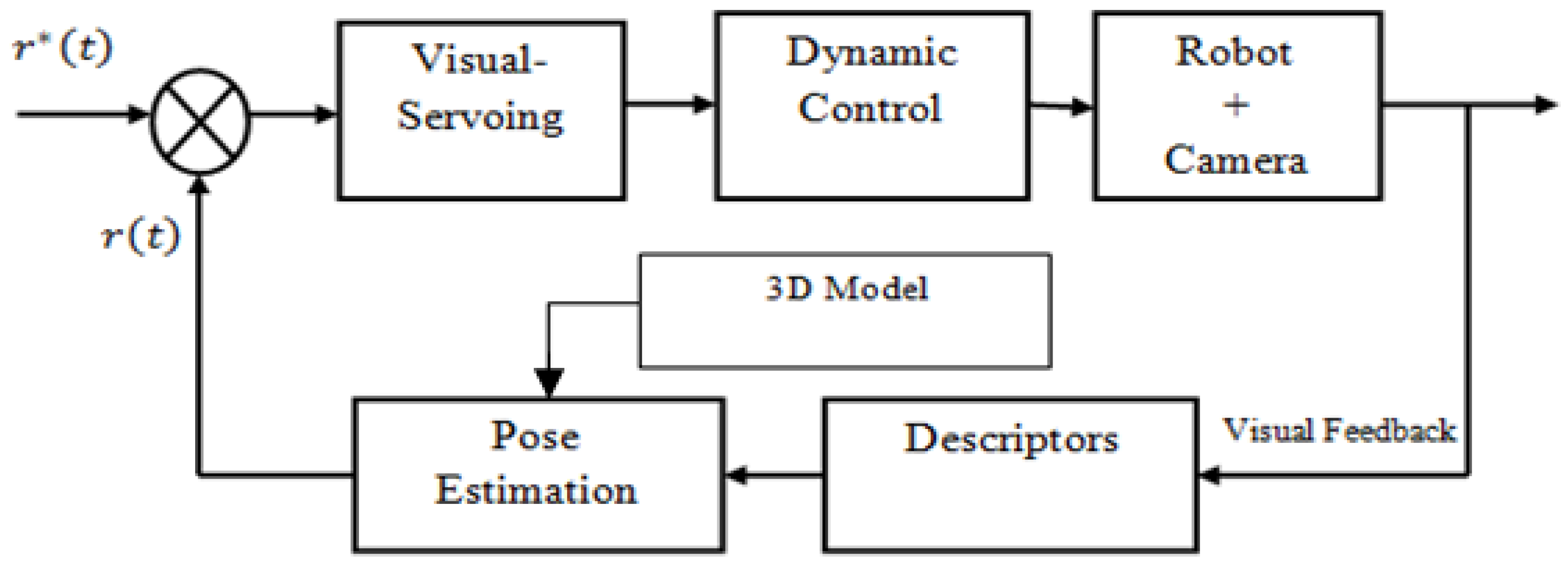
Figure 1. Three-dimensional visual servoing—block diagram.
Applsci 12 06167 g001
Figure 2. Mobile Robot Model.
Applsci 12 06167 g002
Figure 3. Image and Cartesian Coordinate System.
Applsci 12 06167 g003
Figure 4. Neural Network Architecture.
Applsci 12 06167 g004
Figure 5. Translation + Rotation in image space.
Applsci 12 06167 g005
Figure 6. Translation according to xR.
Applsci 12 06167 g006
Figure 7. Translation according to yR.
Applsci 12 06167 g007
Figure 8. Rotation according to zR.
Applsci 12 06167 g008
Figure 9. Example of a proposed trajectory.
Applsci 12 06167 g009
Figure 10. Visual servo control diagram: object does not leave the field of view of the camera.
Applsci 12 06167 g010
Figure 11. Visual servo control diagram: object leaves the field of view of the camera.
Applsci 12 06167 g011
Figure 12. Case 1: Where the object does not leave the field of view of the camera.
Applsci 12 06167 g012
Figure 13. Case 1: Evolution of the robot trajectory in the image plane.
Applsci 12 06167 g013
Figure 14. Case 1: Evolution of the trajectory of the robot in the Cartesian coordinate system.
Applsci 12 06167 g014
Figure 15. Case 1: Evolution of the control law u1.
Applsci 12 06167 g015
Figure 16. Case 1: Evolution of the control law u2.
Applsci 12 06167 g016
Figure 17. Case 2: Where the object leaves the field of view of the camera.
Applsci 12 06167 g017
Figure 18. Case 2: Evolution of the robot trajectory in the image plane.
Applsci 12 06167 g018
Figure 19. Case 2: Evolution of the trajectory of the robot in the Cartesian coordinate system.
Applsci 12 06167 g019
Figure 20. Case 2: Evolution of the control law u1.
Applsci 12 06167 g020
Figure 21. Case 2: Evolution of the control law u2.
Applsci 12 06167 g021
Publisher’s Note: MDPI stays neutral with regard to jurisdictional claims in published maps and institutional affiliations.