
Wavelet Time-Frequency Analysis on Bridge Resonance in Train-Track-Bridge Interactive System


1
School of Civil Engineering, Beijing Jiaotong University, Beijing 100044, China
2
Bridge and Tunnels Department, Russian University of Transport, 127994 Moscow, Russia
*
Author to whom correspondence should be addressed.
Appl. Sci. 2022, 12(12), 5929; https://doi.org/10.3390/app12125929
Submission received: 17 May 2022
/
Revised: 7 June 2022
/
Accepted: 7 June 2022
/
Published: 10 June 2022
(This article belongs to the Special Issue Design of Track System and Railway Vehicle Dynamics Analysis)
Abstract
:With the continuous improvement in the operation speed of trains, the impact of train–induced vibration through the track on the bridge is increasingly prominent. In particular, when the loading frequency is the same as or close to the natural frequency of the bridge, the resonant response of the bridge will be activated, which will probably endanger the safety of the operation and the bridge structure. Normally, the traditional method to indicate the appearance of resonant response is to analyze the frequency spectrum of the response through the Fourier transform from its time history. However, it can simply reflect the contribution of different frequency components within a stationary window. Therefore, continuous wavelet transform is adopted on a 2D train–track–bridge interactive system in this article. It illustrates the evolutionary characteristics of different frequencies from the input excitation to the output response during the bridge resonance in the time–frequency domain, compared with the cases when the bridge is nonresonant. Finally, the article demonstrates the feasibility of the method. It concludes that the resonance and quasi–resonance–triggering band accounts for the highly intensified bridge response, while the staggering domination between the steady-state and the transient response is the main phenomenon for the nonresonant bridge. Additionally, within the low–frequency band, the resonant bridge will have a more significant impact on the track subsystem than the train subsystem.
1. Introduction
The operation of a high–speed train has high requirements for the smoothness and stability of the track, which leads to the dependence on bridge construction, especially in areas with high population density, poor geological conditions and limited land resources. Different from the stationary situation, when the train crosses the bridge at a certain speed, the train and bridge will also vibrate and the system will produce inertial force. The vibration response of the bridge will aggravate the fatigue of its structural members to some extent, resulting in the reduction in its own strength and structural stability [1]. In particular, when the loading frequency corresponding to the train speed is close to the natural vibration frequency of the bridge, the bridge vibration response amplitude will be increased, which may cause damage to itself and endanger driving safety in extreme cases.
Therefore, a comprehensive study on resonant response to ensure the dynamic performance of the bridge and the safety of vehicle operation is conducted at home and abroad to meet the engineering need of railway bridge research and design. Li and Su [2] studied the dynamic response of a girder bridge under high–speed trains, with an emphasis on the resonant vibration, and found that the sum of free–vibration response components generated by each moving load acting successively on the bridge results in the resonance, and if the number of vehicles is very small, resonance may not occur. Kumar et al. [3] proposed a low–cost multi-sensor data acquisition system (DAQ) for detecting various faults in 3D–printed products by using an Arduino micro–controller that collects real–time multi–sensor signals using vibration, current, and sound sensors, which is prospective to the study on scaled resonant bridge models. Ju and Lin [4] investigated the resonant characteristics of three–dimensional bridges when high–speed trains pass them and pointed out that to avoid resonance, the dominated train frequencies and the bridge natural frequencies should be as different as possible, especially for the first dominated train frequency and the first bridge natural frequency in each direction. The resonance mechanism and the conditions of the train–bridge system were investigated by Xia et al. [5] through theoretical derivations, numerical simulations and experimental data analysis. Ülker–Kaustell and Raid Karoumi [6] illustrated the influence of these variations on the train–bridge resonance of this particular bridge by means of a nonlinear single degree of freedom system, based on the previously mentioned experimental results. The results indicate that the influence of the increasing damping ratio leads to a considerable decrease in the resonant amplitude whilst the decreasing natural frequency decreases the critical train speed at which resonance occurs. Considering that the acquisition and transport of sensor data could suffer interference in the train’s environment due to electromagnetic noise from various sources, Pereira et al. [7] presented an architecture for data acquisition of analog data from a train’s environment, drawn to perform data acquisition with various noise sources, which is meaningful for withdrawing the bridge response data from the trains. The Railway Technology Research Centre (CITEF) [8] has developed a new data acquisition system (DAS) based on Odroid which consists of a main box that is compact and easy to transport and will be greatly useful for monitoring comfort and safety in railways during the resonant bridge condition. Matsuoka et al. [9] developed a novel drive–by system for high–speed railways to detect resonant bridges; the difference between two track irregularities at the same position using devices mounted on the first and last vehicles of a train was measured.
With the development of time–analysis theory, an increasing number of applications concerning wavelet transform on train–track–bridge interactive dynamics investigations have been conducted at home and abroad. Ruzzene et al. [10] used the wavelet transform as a time–frequency representation for system identification purposes and confirmed the accuracy of this method by applying it to a numerical example and the acceleration responses from a real bridge under ambient excitation (the Queensborough Bridge in Vancouver, Canada). Piombo et al. [11] described the dynamic tests performed on a simply supported bridge in Northern Italy under traffic excitation and prove that the ability of wavelet transforms to detect abrupt changes, gradual change beginnings and ends of events make them well suited for the analysis of bridge health monitoring data. Moyo et al. [12] present the application of wavelet analysis to identify events and changes in structural state in a bridge during and after its construction. Meo et al. [13] showed the capabilities of the real–time kinematic (RTK) global positioning network system (GPS) to measure the low–frequency vibration of a medium–span suspension bridge. The traditional method of attaching strain transducers to the soffit of the bridge and placing axle detectors on the road surface has been replaced here by using additional transducers underneath the bridge for axle detection and nothing–on–the–road (NOR). Chatterjee et al. [14] presented a wavelet–based analysis of strain signals and showed the efficacy of using wavelets in pattern recognition of these signals. An algorithm based on a plot of wavelet coefficients versus time to detect damage appears to be very sensitive to noise. Hester et al. [15] addressed these questions by: (a) using the acceleration signal, instead of the deflection signal, (b) employing a vehicle–bridge finite element interaction model, and (c) developing a novel wavelet–based approach using wavelet energy content at each bridge section, which proves to be more sensitive to damage than a wavelet coefficient line plot at a given scale as employed by others. Pacheco–Chérrez et al. [16] described a completely new method based on modal analysis to locate and also measure the length and orientation of crack–type damage features in thin–walled composite beams (TWCB). It was found that the method is useful for the measurement of damage features in a variety of thin–walled composite beams such as aircraft wings and wind turbine blades, among others.
In spite of plenty of research mentioned above, there is still a lack of comprehensive time–frequency characteristics analysis on bridge resonance for how the frequency component for the input excitation evolves as time goes by, how the bridge response transits from the nonresonant to resonant condition in the time–frequency domain and how the resonant bridge reacts on the track and the train subsystems. In this case, the article will establish a 2D train–track–bridge interactive model based on the wavelet computational properties, clarify the time–frequency characteristics from the input excitation to the output response through the comparison among a nonresonant, resonantly transitional, and resonant bridge, and analyze the resonant reaction from the bridge on the track and the train subsystem.
2. Establishment and Solution of Motion Equation for Train–Track–Bridge Interactive System Based on Wavelet Computational Properties
2.1. Wavelet Time-Frequency Analysis Theory and Relevant Computational Deduction
Similar to the Fourier transform, the trigonometric function is used as the basis function to compare the time–domain signal. On the premise of assuming , the basis function in the wavelet transform meets the condition , where the Fourier transform of is . The wavelet base is expanded and translated, and its expansion factor (also known as the scale factor) is a, the translation factor is b, and the function after translation and expansion is , which is expressed as Equation (1) [17].
For the signal , its continuous wavelet transform (CWT) is expressed as Equation (2) [17].
Simultaneously, the inverse continuous wavelet transform (ICWT) to reconstruct the signal can be expressed as Equation (3) [17].
Essentially speaking, the wavelet decomposition is to constantly change the center (real–time translation) and scale of the wavelet window, multiply it with the signal for integral operation, compress the scale at high frequency and stretch the scale at low frequency, so as to obtain the signal component at any time under each frequency scale. Generally, the CWT spectrum can be defined as scalogram in Equation (4), a type of signal energy distribution with the translation factor b and the scale factor a.
According to Parseval’s theorem [18], the weighted integral of the amplitude square of wavelet transform on the scale–translation plane (a − b) is equal to the total energy of the signal in the time domain, shown in Equation (5). Therefore, the amplitude square of wavelet transform can be regarded as a representation of the time–frequency distribution of signal energy.
The key to wavelet transform is the selection of wavelet basis function. The smaller the time domain window width is, the stronger the time domain analysis ability of the wavelet basis is. Similarly, the smaller the frequency domain window width, the stronger the frequency domain analysis ability of the wavelet base is. The bump wavelet [18] selected in this paper has small variance in the frequency domain and high frequency resolution, which can avoid energy leakage in the process of frequency conversion and be expressed in Equation (6) [19].
where is the indicator function, μ and σ are the wavelet base parameters, and the effective interval μ is [3, 6]. The effective interval of σ is [0.1, 1.2]. As for smaller σ, the wavelet has good frequency resolution, but poor time resolution. As for larger σ, it produces wavelets with better time resolution and poorer frequency resolution. Generally, in the program, the default values for μ and σ are 5 and 0.6, respectively. The time history and frequency domain laws of the wavelet are shown in Figure 1.
Moreover, the wavelet computational properties are of great significance to the establishment of motion equations in the time–frequency domain and mainly includes the linearity, the time translation, the derivation and the approximation. Their definitions and deductions are listed as follows.
As for linearity, x(t) and y(t) are supposed to be two signals linearly formulating signal z = kx + cy with constant coefficients k and c. In this case, the wavelet transform of signal z can be expressed in Equation (7) by the linear superposition of the wavelet transforms of x and y.
As for the time translation, x(t) and y(t) are supposed to be two signals and y(t) can be defined by the x(t) with a delay factor τ, namely y(t) = x(t − τ). In this case, the wavelet transform of signal y can be expressed in Equation (8) by the consistent translation for the translation factor b within the wavelet transform of x.
As for the derivation, x(t) and y(t) are supposed to be two signals and y(t) is the first–order derivative of time for x(t), namely y(t) = dx/dt. In this case, the wavelet transform of signal y can be expressed in Equation (9) by the derivation of translation factor b within the wavelet transform of x.
As for the approximation, x(t) and y(t) are supposed to be two signals formulating signal z = xy through the element–wise product with x(t) = A(t), namely, slowly varying the modulating function and y(t) = exp(jφ(t)), namely the phase time–varying function. In this case, signal z can be regarded as an asymptotic signal if oscillation due to the phase term φ(t) is more than that contributed by the amplitude term A(t) [20]. Correspondingly, the wavelet transform of signal z can be approximated in Equation (10) by the multiplication of the wavelet transform of x and the original signal y.
2.2. Establishment of Motion Equation for the Train Subsystem
The train subsystem is modeled by several independent vehicle elements shown in Figure 2, each of which includes a car body, two bogies, four wheel sets, and a two–layer spring–damper suspension system by referring to Table 1. The assumptions are made to simplify the analysis with enough accuracy. Namely, the interaction is neglected among vehicle elements. The rigid car body, bogies, and wheel sets in each vehicle element are adopted. The vehicle element is a linear system; namely, the mass, damping, and stiffness matrices of the vehicle element are constant. The train runs on the track at a constant speed. The wheels and rails fit snugly. In this way, each vehicle element includes six independent degrees of freedom (DOFs) for the car body (zci, φci) and bogies (zb1i, φb1i, zb2i, φb2i), and with four dependent DOFs (zw1i, zw2i, zw3i, zw4i) for the wheel sets reflecting the vertical motion states of four contact points, where z is the vertical displacement; φ is the pitch torsional displacement; the numbers of the bogies and the wheel sets represent the front and rear orders; and subscript i denotes the order of certain vehicle elements.
In accordance with the D’Alembert principle, the motion equation of the train can be established in Equation (11).
where Mt, Ct, Kt and Tt signify, respectively, the mass, the damping, the stiffness and projector matrices of the train and can be formulated by diagonally assembling the Mve, Cve, Kve and Tve of vehicle elements in the same way as Equation (13). Similar to Kve in Equation (14), Cve can be formulated by replacing the spring factor k with damping factor c.
With the application of CWT in Equation (2) and its computational properties of linearity and derivation in Equations (7) and (9), the motion equation of the train can be redefined as Equation (16) in the CWT domain.
2.3. Establishment of Motion Equation for the Track–Bridge Subsystem
The track–bridge subsystem is presented in Figure 3 with three layers containing the rail, sleepers and bridges from top to bottom, between two of which there is an inserted connective layer of spring–dampers simulating fasteners and ballasts, respectively. For the specific meaning of the parameters, refer to Table 2; they are selected according to the mainstream parameters in the world for the track–bridge subsystem.
In detail, the rail and the bridges with simple support are modeled by the finite element method (FEM) with multiple Euler beam elements, each of which includes four DOFs (left node: zj, φj; right node: zj+1, φj+1) and considers the Raylewigh damping [22]. Furthermore, the sleepers are modeled as rigid bodies, each of which vibrates with only one vertical DOF. According to the FEM, the shape function will be adopted to interpolate the layers of the fasteners (rail to sleepers) and the ballasts (sleepers to bridges), respectively, in the way of non–nodal connection so as to simplify the model by reducing the DOFS of rail and bridges.
In accordance with the D’Alembert principle, the motion equation of the train can be established in Equations (17) and (18).
The mass matrix Mb and stiffness matrix Kb of the bridge can be formed by withdrawing the nonsupport elements from the matrix Kbe10 and Mbe10 assembled in the way of Equation (18) with Mbe and Kbe for beam elements. Based on Raleigh damping, the damping matrix Cb of the bridge can be expressed in Equation (17) by combination of Mb and Kb with ξb, damping ratio of the bridge, and ωb1 and ωb2, the first and second order angular frequencies of the bridge, respectively. The formulation of Mr, Kr and Cr for the rail can be conducted by similar means to the bridge.
Moreover, Krs and Crs, the transpose of which are Ksb and Csb, reflect in Equation (17) the interaction of layers and are formulated through the interpolation of the shape function which can be expressed in Equation (23) with the local distance x on a certain bridge or rail element.
Therefore, as for the substructure in Figure 3b, the fasteners–ballasts stiffness contributing matrix Kfb can be defined in Equation (24) where the main diagonal elements are added to Kr, Ks and Kb while the remaining elements are added to Krs and Ksb as well as their transpose within the corresponding positions of the track–bridge stiffness matrix. Simultaneously, the damping matrix in Equation (17) follows the same definition as above.
![Applsci 12 05929 i001]()

Tr in Equation (18) is the decomposition matrix to project the wheel–rail force to the nodes of the beam elements contacted by the wheel sets. As a submatrix, Trve in Tr can be sequenced as subvectors τrw for four wheel sets in a vehicle element. The time difference among four wheel sets in a vehicle element distinguishes τrw in Equation (26) by subtraction of time delay and in Equation (21). The subfunction P defined through the shape function in Equation (23) projects the wheel–rail force, respectively, to the vertical DOF in Equation (28) and to the pitch torsional DOF in Equation (29).
With the application of CWT in Equation (2) and its computational properties of linearity and derivation in Equations (7) and (9), the motion equation in Equation (17) of the track–bridge subsystem can be redefined as Equation (30) in the CWT domain.
According to the wavelet computational property of approximation and wheel–rail tight fitting assumption, the CWT of the wheel–rail contact vibratory displacement can be defined in Equation (32) where zir is the track irregularity vector for the wheel sets, which helps to deduce Equation (31) to the approximated form in Equation (33).
Commonly, the definition of track irregularity time series follows the trigonometric series superposition method. Therefore, the expression of track irregularity can be defined in Equation (34). Owing to the phase delay between every two wheel sets, the CWT of track irregularity in Equation (35) passed by every wheel set can be simplified through wavelet translation for the first wheel set track irregularity property in Equation (8).
where td is the delay vector for each wheel set, Sv is the given vertical track irregularity PSD, nk is an angular wave number sample, dn is the bandwidth, and θk is a random phase angle obeying the uniform distribution U(0,2π). The integer order of k ranges from 1 to N2. Relevant parameters can refer to Equation (36), namely the German vertical track irregularity power spectrum density [23], and Table 3.
2.4. Intersystem Iteration Solution Procedures
The intersystem iteration method [24], also called as the whole–process iteration method, is a newly developed method to solve the train–track–bridge motion equation. At present, the train–track–bridge motion equation has been redefined by CWT, respectively, in Equations (16) and (30) and separated to be two stationary linear subsystems, namely, the train and track–bridge. Therefore, the intersystem iteration method is suitable for the solution in the CWT domain through linear integration of its translation factor b by the Newmark–β method, a type of time history integration method. In detail, the procedures can be extended in Figure 4.
Firstly, with the CWT of track irregularity input as the wheel set motion and under the assumption of the initially rigidized track–bridge subsystem, the CWT of the train response and the wheel–rail force can be calculated through the solution of independent train motion equations. Secondly, the CWT of the wheel–rail forces is applied to the rail; thus, the motion state CWT of the track–bridge subsystem can be obtained through the solution of the independent bridge equation. Thirdly, the next iteration is carried out by the superposition of the calculated deck motion CWT with the track irregularities CWT as an updated train subsystem excitation. The signal energy of the wheel–rail force calculated by Equation (5) can also be adopted as the index for the convergence judgment. When the absolute error of signal energy between the former and the present iteration is smaller than 10%, the procedure is judged to be convergent. Finally, the output will be implemented, followed by the end of the procedure.
3. Time-Frequency Interaction Analysis on the Train–Track–Bridge System
3.1. Analysis of Methodological Correctness
This section will demonstrate the methodological correctness through the inverse CWT on the vibratory acceleration of the car body and the mid–span of the bridge, compared with the results obtained by traditional integration. Based on the parameters in Table 1, Table 2 and Table 3, the train is simulated to run on the track–bridge system at a speed of 350 km/h.
Through the comparison in Figure 5, it is found that the response history curve, respectively, by the CWT–ICWT method and traditional time history integration method is of significant consistency; therefore, the integration based on CWT to realize the conversion from excitation to response is proved to be feasible and can be adopted to the following time–frequency analysis.
3.2. Division of the Band from Resonant to Nonresonant Bridge Condition
In order to study the preconditions of resonance and accurately describe the time–frequency evolutionary characteristics of resonant, nonresonant and resonantly transitional bridge response, several speed conditions were firstly selected within the range of 90–720 km/h, which helps to determine the mid–span bridge vibratory acceleration signal energy calculated by Equation (5) in the function of train speed shown in Figure 6.
Secondly, the bridge natural frequency is 6.5 Hz according to Table 2. The theoretical resonant speeds (195, 292.5 and 585 km/h) were determined with the arrow in Figure 6 according to first–order loading frequencies (train speed/vehicle length, namely V/lv; 2.17, 3.25 and 6.5 Hz) which is equal to 1/n (n is integer) time of the bridge natural vibration frequency. It can be seen in the Figure that the component of 585 km/h dominates the bridge acceleration signal energy, which reflects that the bridge vibrates the most intensely when the first–order loading frequency is identical to the bridge natural frequency.
Thirdly, the speed ranges in blue are defined as the resonantly transitional band through the gradient of signal energy. Their limits are marked according to the relative percentage to the theoretical resonant speeds. The reason why the resonantly transitional band is not allocated to the theoretical speed of 292.5 km/h is because there is no significant fluctuation in bridge vibratory acceleration signal energy around this speed.
3.3. Time-Frequency Analysis from Excitation to Bridge Response
3.3.1. On the Resonant Bridge
In order to study the time–frequency evolutionary characteristics on the resonant bridge from excitation to response, the speed conditions of 195, 292.5 and 585 km/h were selected, and the corresponding first–order loading frequencies are 2.17, 3.25 and 6.5 Hz, respectively. The CWT scalograms of mid–span bridge excitation and vertical acceleration response are shown in Figure 7 and it can be seen that:
- For the excitation scalogram in Figure 7a,c,e, there are only three loading frequency orders in yellow under all the speed conditions, reflecting that the influence of higher–order loading frequency is basically negligible. Frequency values of each order are integer multiples of the first–order loading frequency, respectively, while the order with the frequency band equal to the bridge natural frequency (6.5 Hz) is defined as the resonance–triggering band. Among them, the first–order loading frequency is the largest, containing the highest signal energy, followed by the third–order and second–order. The scalogram value corresponding to each loading frequency order firstly increases and then decreases with the process of entering and leaving the bridge. The scalogram value of each loading frequency order will not change with the increase in speed, but its frequency and the bandwidth between each order frequency will increase with the increase in speed.
- For the response scalogram in Figure 7d, the triggered resonance band, corresponding to the second–order response frequency, is not completely dominant for the entire response with the existence of other orders of response frequency. In contrast, for Figure 7b,e, only the triggered resonance bands are visible and completely dominate the entire response. The scalogram value of the triggered resonance band in Figure 7b is more significant than the one in Figure 7e.
- In general, the bridge resonant response is stationary while the train is crossing the bridge. The resonance–triggering band is included within each order of loading frequency, while the triggered resonance band will dominate the bridge response only when the signal energy of the corresponding triggering band is significant. Typically, the resonance–triggering band which is in the first–order loading frequency and equals the natural frequency of bridge will lead to the most intense bridge resonant response.
3.3.2. On the Resonantly Transitional Bridge
In order to study the time–frequency evolutionary characteristics on the resonantly transitional bridge from excitation to response, the speed conditions of 175, 210 and 550 and 680 km/h were selected, and the corresponding first–order loading frequencies are 1.94, 2.33, 6.11 and 7.56 Hz, respectively, according to the division in Figure 6 of Section 3.2. The CWT scalograms of mid–span bridge excitation and vertical acceleration response are shown in Figure 8 and it can be seen that:
- For the excitation scalogram in Figure 8a,c,e,g, the time–frequency band distributive regulations are almost identical to Section 3.3.1. The frequency band circled in white is defined as the quasi–resonance–triggering band because the frequency components within this band are close to the bridge natural frequency (6.5 Hz).
- For the response scalogram in Figure 8b,d,f,h, the triggered quasi–resonance bands completely dominate the entire response because they are close to the bridge natural frequency. Simultaneously, the sorting of scalogram values in descending order is listed as (f) > (h) >> (b) > (d).
- In general, the bridge’s resonantly transitional response is stationary while the train is crossing the bridge. The quasi–resonance–triggering band is included within each order of loading frequency and in this case, the triggered quasi–resonance band will dominate the bridge response. Typically, the closer the quasi–resonance–triggering band is to the natural frequency of the bridge, the more the bridge resonant response will be intensified. Therefore, reasonably controlling train speed can crucially help to keep the bridge away from intense quasi–resonant response.
3.3.3. On the Nonresonant Bridge
In order to study the time–frequency evolutionary characteristics on the nonresonant bridge from excitation to response, the speed conditions of 320, 350 and 400 km/h were selected, and the corresponding first–order loading frequencies are 3.56, 3.89 and 4.44 Hz, respectively. The CWT scalograms of mid–span bridge excitation and vertical acceleration response are shown in Figure 9 and it can be seen that:
- For the excitation scalogram in Figure 9a,c,e, the time–frequency band distributive regulations are almost identical to Section 3.3.1 and Section 3.3.2. Owing to the train speed which is situated in the nonresonant bridge condition according to Figure 6 in Section 3.2, the quasi–resonance and resonance–triggered band disappears from the excitation scalogram.
- For the response scalogram in Figure 9b,d,f, there is a “peak staggering” phenomenon between the transient response band and the steady state response band. During this period, the first wheel set of the vehicle acts on the bridge which has no time to produce a steady state response, so free vibration whose frequency equals the bridge natural frequency will occur within the transient response band. When the moving load becomes stably periodic, the bridge presents a steady state response, and the scalogram value will increase to the first–order response frequency contributed by the first–order loading frequency, while the scalogram value is attenuated in the transient response band. At the moment when the last wheel set leaves the bridge, with the end of wheel set periodic loading, the steady state response weakens and is gradually replaced by the transient response. Therefore, a higher scalogram value is reintensified in the transient response band after the train leaves the bridge. With the increase in train running speed, the scalogram values of steady state response and transient response are slightly higher than those under low–speed conditions.
- In general, the nonresonant response of the bridge is mainly composed of the steady–state response contributed by the loading frequency component, while the transient response is contributed by the bridge natural vibration frequency. The response is steady state when the train moves on the bridge and transient at the initial stage and later stage of the train entering and leaving the bridge. In addition, the intensity of nonresonant response of the bridge is related to the train speed.
3.4. Evolutionary Reaction Analysis from the Bridge on the Track and the Train Subsystem
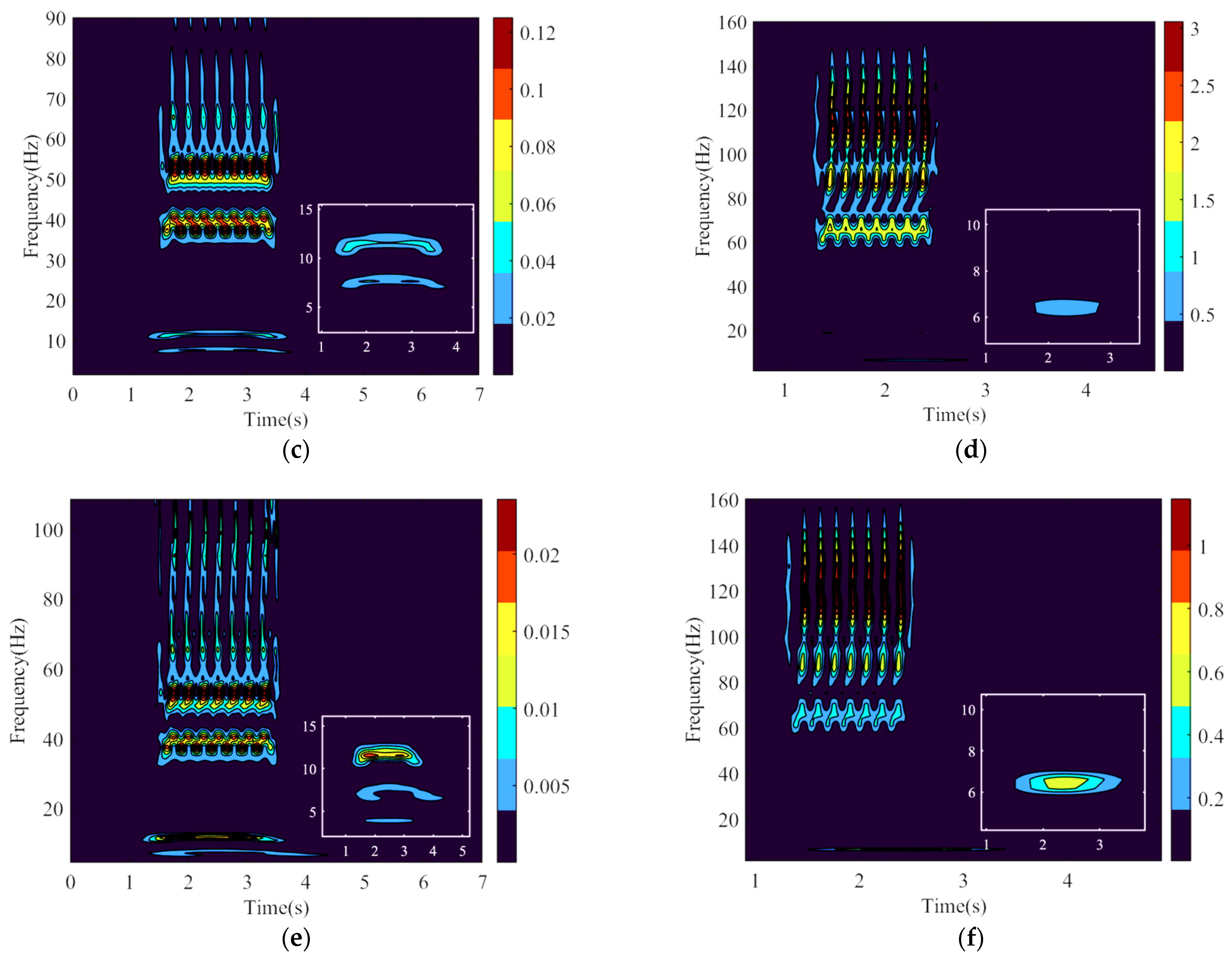
In order to study the time–frequency evolutionary characteristics on the internal reaction from the bridge subsystem on the track and the train, the speed conditions of 350 and 585 km/h were selected, respectively, corresponding to the nonresonant and resonant bridge conditions, and the corresponding first–order loading frequencies are 3.89 and 6.50 Hz, respectively. The CWT scalograms of the first car body, one of the mid–sleepers, and mid–rail vertical acceleration response are shown in Figure 10:
- By comparison, between Figure 10a,b, the frequency band for the car body response is extremely scattered and there is no significant and stable time–frequency band which can clearly present the stable bridge natural frequency (6.5 Hz). In contrast, it can only be seen that the scalogram value increases with the increase in the train speed which is positively correlated to the velocity and the acceleration of track irregularity. Therefore, the car body response is dominated by the track irregularity excitation which has masking effect on the bridge response.
- By comparison between Figure 10c,d, the high frequency band for the mid–rail presents the multiple peaks fluctuating phenomenon, which signifies the periodic loading process conducted by the continuous movement of multiple vehicle elements. Simultaneously, with the increase in train speed, the former high frequency band will move upwards to a higher frequency band. In terms of the low frequency band within the sub–windows, both of them contain the components of bridge natural frequency, which signifies that the feedback comes from the bridge response and in particular, will be intensified under the bridge resonant condition.
- Figure 10e,f share the similar time–frequency characteristics to (c) and (d). The feedback which comes from the bridge response will be intensified under the bridge resonant condition. Particularly, the sleepers are closer to the bridge than the rail; therefore, the feedback on the sleepers is more intense than that on the rail.
- In general, within the low–frequency band, the resonant bridge will have a more significant impact on the track subsystem, especially for the substructure closer to the bridge deck, than the nonresonant one, while the impacts from the bridges almost neglect the car body.
4. Discussion
The article mainly focuses on applying the wavelet time–frequency analysis to the initial study on the bridge resonance in a simple train–track–bridge interactive model. Therefore, to some extent, there exists a certain amount of limitations and deficiency which needs to be improved for the future scope of study.
- The train–track–bridge interactive model established in the article is 2D, only involving the vertical displacement and the torsional pitching. Hence, to make the results closer to the realistic project, the study will be extended in a 3D train–track–bridge interactive model with more DOFs.
- The article is lacking in the data measured on site to validate the theoretical results and rectify the model. Thus, the future study will try to launch the real measurement both on the train and on the bridge.
- The article neglects that the track irregularity is actually a type of random excitation which will randomize the response of the train–track–bridge interactive system. In this case, the future study will combine the random vibration theory with the wavelet time–frequency analysis so as to make this method feasible for the actual damage detection on the train–track–bridge interactive system.
5. Conclusions
This article has established the initial system for the time–frequency analysis on the bridge resonant response in a train–track–bridge interactive system based on continuous wavelet transform and its computational properties. The direct integration through an intersystem iteration solution is adopted on the translation factors and realizes the conversion from excitation to response in the wavelet domain, which is proved feasible and precise in time–frequency evolutionary characteristic analysis. Relevant conclusions can be drawn as follows:
- The bridge resonant response is stationary while the train is crossing the bridge. The resonance–triggering band is included within each order of loading frequency, while the triggered resonance band dominates the bridge response only when the signal energy of the corresponding triggering band is significant. Typically, the resonance–triggering band, which is located in the first–order loading frequency and equals the natural frequency of bridge, will lead to the most intense bridge resonant response.
- The bridge’s resonantly transitional response is stationary while the train is crossing the bridge. The quasi–resonance–triggering band is included within each order of loading frequency and will dominate the bridge response. Typically, the closer the quasi–resonance–triggering band is to the natural frequency of bridge, the more the bridge response will be intensified.
- The nonresonant response of the bridge is mainly composed of the steady state response contributed by the loading frequency component and the transient response contributed by the bridge natural vibration frequency. The response is steady state when the train moves on the bridge forming periodic loading, while transient at the initial stage and later stage of the train entering and leaving the bridge. Staggering domination between the steady state and the transient response is the main phenomenon for the nonresonant bridge.
- Within the low–frequency band, the resonant bridge will have more significant impact on the track subsystem, especially for the substructure closer to the bridge deck, than the nonresonant one, while the impacts from the bridges almost neglect the car body even under the resonant bridge condition.
Author Contributions
Z.W. came up with the concept, realized the simulation, analyzed the data and edited the draft of manuscript. N.Z. conducted the literature review, checked the computations, wrote the draft of the manuscript, replied to reviewers’ comments and revised the final version. J.Y. verified the simulated data and polished the article. V.P. corrected the model of simulation and debugged the programming. All authors have read and agreed to the published version of the manuscript.
Funding
National Natural Science Foundation of China, Grant number: 52178101.
Institutional Review Board Statement
Not applicable.
Informed Consent Statement
Not applicable.
Data Availability Statement
The data presented in this article are available on request from the corresponding author.
Acknowledgments
Thanks for the support for this work from the National Natural Science Foundation of China.
Conflicts of Interest
The authors declare no conflict of interest.
References
- Xia, H.; Zhang, N.; Guo, W. Dynamic Interaction of Train-Bridge Systems in High-Speed Railways; Springer: Berlin/Heidelberg, Germany, 2018. [Google Scholar] [CrossRef]
- Li, J.; Su, M. The resonant vibration for a simply supported girder bridge under high-speed trains. J. Sound Vib. 1999, 224, 897–915. [Google Scholar] [CrossRef]
- Kumar, S.; Kolekar, T.; Patil, S.; Bongale, A.; Kotecha, K.; Zaguia, A.; Prakash, C. A Low-Cost Multi-Sensor Data Acquisition System for Fault Detection in Fused Deposition Modelling. Sensors 2022, 22, 517. [Google Scholar] [CrossRef] [PubMed]
- Ju, S.; Lin, H. Resonance characteristics of high-speed trains passing simply supported bridges. J. Sound Vib. 2003, 267, 1127–1141. [Google Scholar] [CrossRef]
- Xia, H.; Zhang, N.; Guo, W. Analysis of resonance mechanism and conditions of train–bridge system. J. Sound Vib. 2006, 297, 810–822. [Google Scholar] [CrossRef]
- Ülker-Kaustell, M.; Karoumi, R. Influence of non-linear stiffness and damping on the train-bridge resonance of a simply supported railway bridge. Eng. Struct. 2012, 41, 350–355. [Google Scholar] [CrossRef]
- Pereira, A.; Pimentao, J.P.; Sousa, P.; Onofre, S. Smart sensor data acquisition in trains. In Proceedings of the 43rd Annual Conference of the IEEE Industrial Electronics Society, Beijing, China, 29 October–1 November 2017; pp. 5598–5603. [Google Scholar] [CrossRef] [Green Version]
- Cano-Moreno, J.D.; De Pedro, J.M.M.S.; Villagrá, M.R.; Gil González, R. Design and development of a data acquisition system to monitor comfort and safety in railways. Insight-Non-Destr. Test. Cond. Monit. 2021, 63, 47–54. [Google Scholar] [CrossRef]
- Matsuoka, K.; Tanaka, H.; Kawasaki, K.; Somaschini, C.; Collina, A. Drive-by methodology to identify resonant bridges using track irregularity measured by high-speed trains. Mech. Syst. Signal Process. 2021, 158, 107667. [Google Scholar] [CrossRef]
- Ruzzene, M.; Fasana, A.; Garibaldi, L.; Piombo, B. Natural Frequencies and Dampings Identification Using Wavelet Transform: Application to Real Data. Mech. Syst. Signal Process. 1997, 11, 207–218. [Google Scholar] [CrossRef]
- Piombo, B.; Fasana, A.; Marchesiello, S.; Ruzzene, M. Modelling and Identification of The Dynamic Response of A Supported Bridge. Mech. Syst. Signal Process. 2000, 14, 75–89. [Google Scholar] [CrossRef]
- Moyo, P.; Brownjohn, J. Detection of anomalous structural behaviour using wavelet analysis. Mech. Syst. Signal Process. 2002, 16, 429–445. [Google Scholar] [CrossRef] [Green Version]
- Meo, M.; Zumpano, G.; Meng, X.; Cosser, E.; Roberts, G.; Dodson, A. Measurements of dynamic properties of a medium span suspension bridge by using the wavelet transforms. Mech. Syst. Signal Process. 2006, 20, 1112–1133. [Google Scholar] [CrossRef]
- Chatterjee, P.; Obrien, E.; Li, Y.; González, A. Wavelet domain analysis for identification of vehicle axles from bridge measurements. Comput. Struct. 2006, 84, 1792–1801. [Google Scholar] [CrossRef] [Green Version]
- Hester, D.; Gonzalez, A. A wavelet-based damage detection algorithm based on bridge acceleration response to a vehicle. Mech. Syst. Signal Process. 2012, 28, 145–166. [Google Scholar] [CrossRef] [Green Version]
- Pacheco-Chérrez, J.; Cárdenas, D.; Probst, O. Measuring Crack-type Damage Features in Thin-walled Composite Beams using De-noising and a 2D Continuous Wavelet Transform of Mode Shapes. J. Appl. Comput. Mech. 2020, 7, 355–371. [Google Scholar] [CrossRef]
- Jiang, Q.; Suter, B.W. Instantaneous frequency estimation based on synchrosqueezing wavelet transform. Signal Process. 2017, 138, 167–181. [Google Scholar] [CrossRef]
- Chang, H.-H. Non-intrusive fault identification of power distribution systems in intelligent buildings based on power-spectrum-based wavelet transform. Energy Build. 2016, 127, 930–941. [Google Scholar] [CrossRef]
- Choose a Wavelet [DB/OL]. 2020. Available online: https://www.mathworks.com/help/wavelet/gs/choose-a-wavelet.html#d120e1132 (accessed on 16 May 2022).
- Staszewski, W.J.; Wallace, D.M. Wavelet-based Frequency Response Function for time-variant systems—An exploratory study. Mech. Syst. Signal Process. 2014, 47, 35–49. [Google Scholar] [CrossRef]
- Zhang, N.; Zhou, Z.; Wu, Z. Safety evaluation of a vehicle–bridge interaction system using the pseudo-excitation method. Railw. Eng. Sci. 2021, 30, 41–56. [Google Scholar] [CrossRef]
- Xiang, J.; Jiang, Z.; Chen, X. A class of wavelet-based Rayleigh-Euler beam element for analyzing rotating shafts. Shock. Vib. 2011, 18, 447–458. [Google Scholar] [CrossRef]
- Xiang, J.; Li, D.-J.; Zeng, Q.-Y. Simulation of spatially coupling dynamic response of train-track time-variant system. J. Central South Univ. Technol. 2003, 10, 226–230. [Google Scholar] [CrossRef]
- Zhang, N.; Xia, H. A Vehicle-Bridge Interaction Dynamic System Analysis Method Based on Inter-System Iteration. China Railw. Sci. 2013, 34, 32–38. [Google Scholar] [CrossRef]
Figure 1.
Definition of bump wavelet: (a) History of bump wavelet; (b) Time–frequency spectra of bump wavelet.
Figure 1.
Definition of bump wavelet: (a) History of bump wavelet; (b) Time–frequency spectra of bump wavelet.
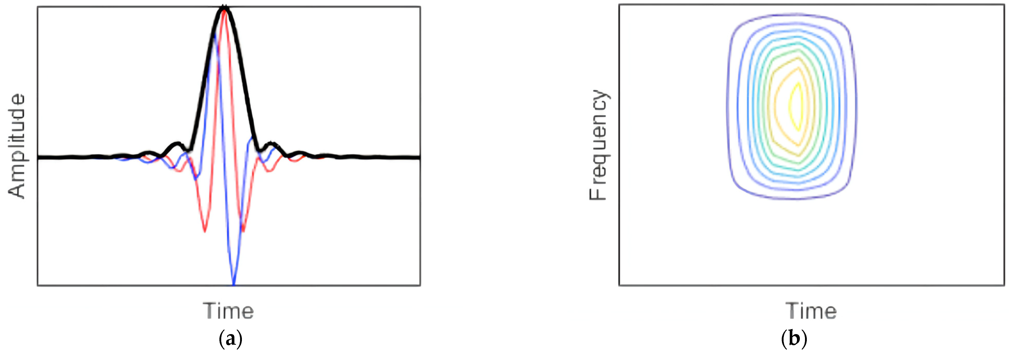
Figure 2.
2D model of the vehicle element.

Figure 3.
2D model of track–bridge subsystem: (a) Global view of 2D model of track–bridge subsystem; (b) Beam element j; (c) Local view of track–bridge subsystem.
Figure 3.
2D model of track–bridge subsystem: (a) Global view of 2D model of track–bridge subsystem; (b) Beam element j; (c) Local view of track–bridge subsystem.

Figure 4.
Flowchart of intersystem iteration procedure.
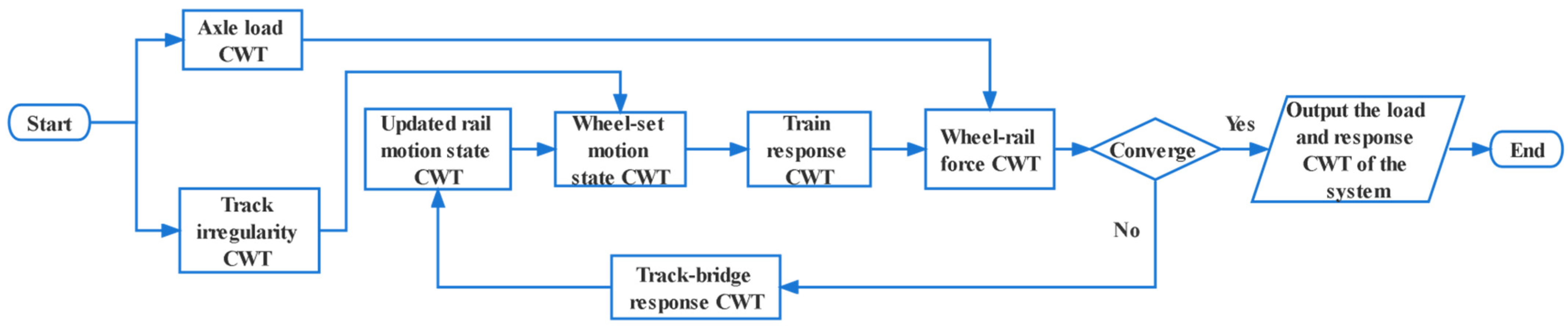
Figure 5.
Comparison of response history between CWT–ICWT method and traditional time history integration method: (a) Response history of car body vertical acceleration; (b) Response history of bridge mid–span vertical acceleration.
Figure 5.
Comparison of response history between CWT–ICWT method and traditional time history integration method: (a) Response history of car body vertical acceleration; (b) Response history of bridge mid–span vertical acceleration.
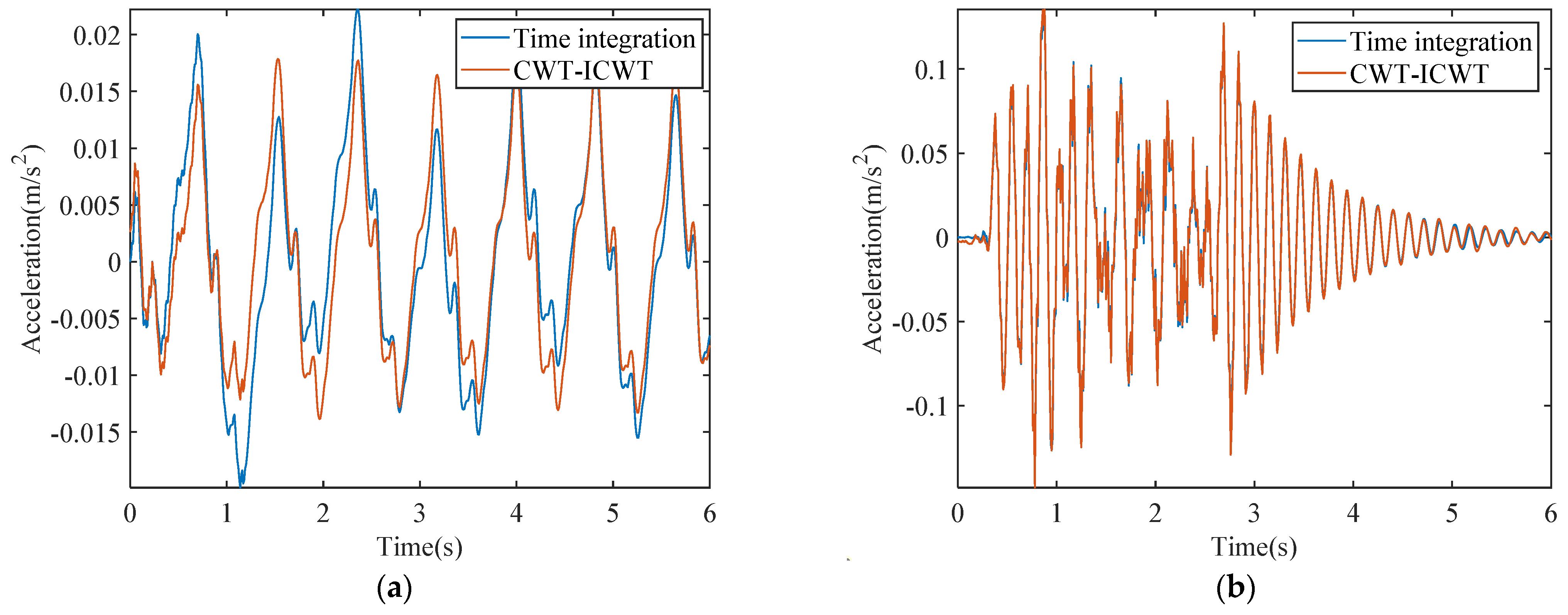
Figure 6.
Mid–span bridge vertical vibratory acceleration signal energy in the function of train speed: (a) Local view; (b) Global view.
Figure 6.
Mid–span bridge vertical vibratory acceleration signal energy in the function of train speed: (a) Local view; (b) Global view.
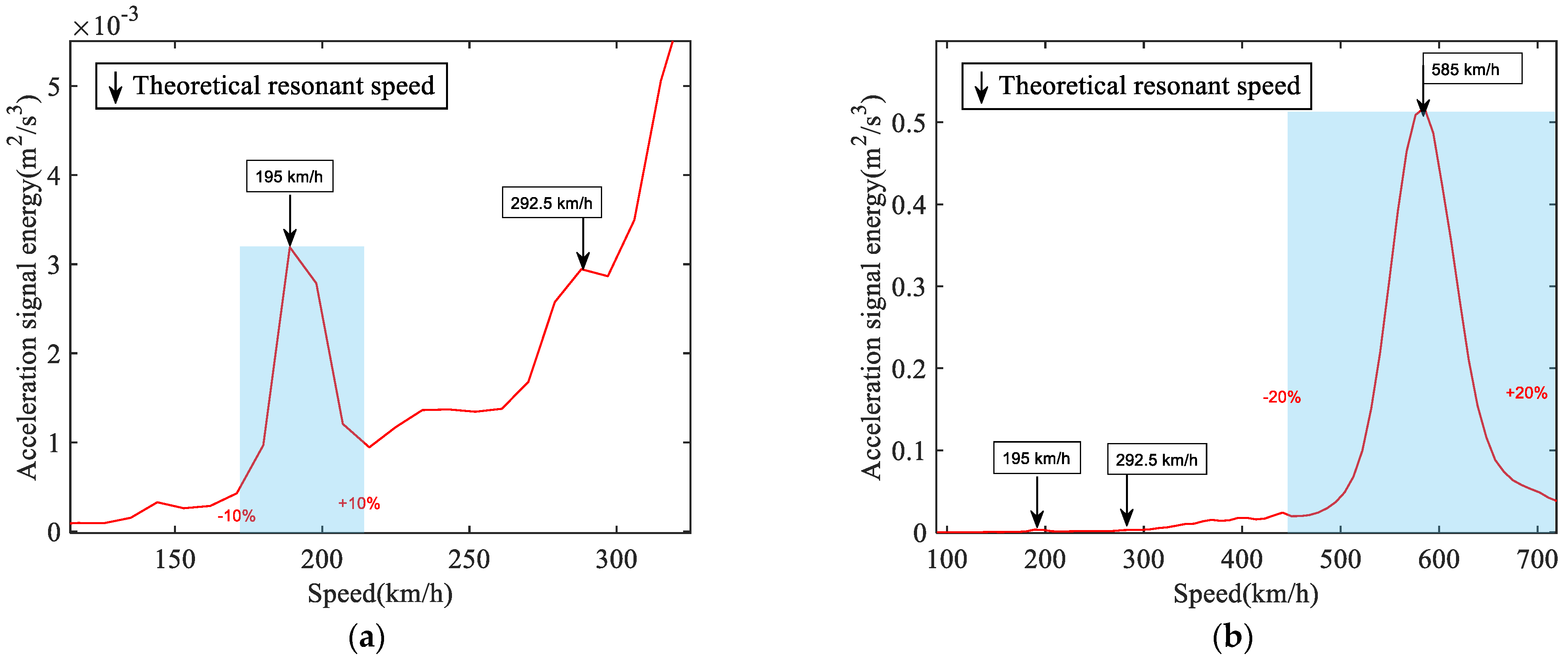
Figure 7.
Scalogram from excitation to vertical vibratory resonant acceleration response at mid–span bridge: (a) Excitation scalogram at 195 km/h; (b) Bridge response scalogram at 195 km/h; (c) Excitation scalogram at 292.5 km/h; (d) Bridge response scalogram at 292.5 km/h; (e) Excitation scalogram at 585 km/h; (f) Bridge response scalogram at 585 km/h.
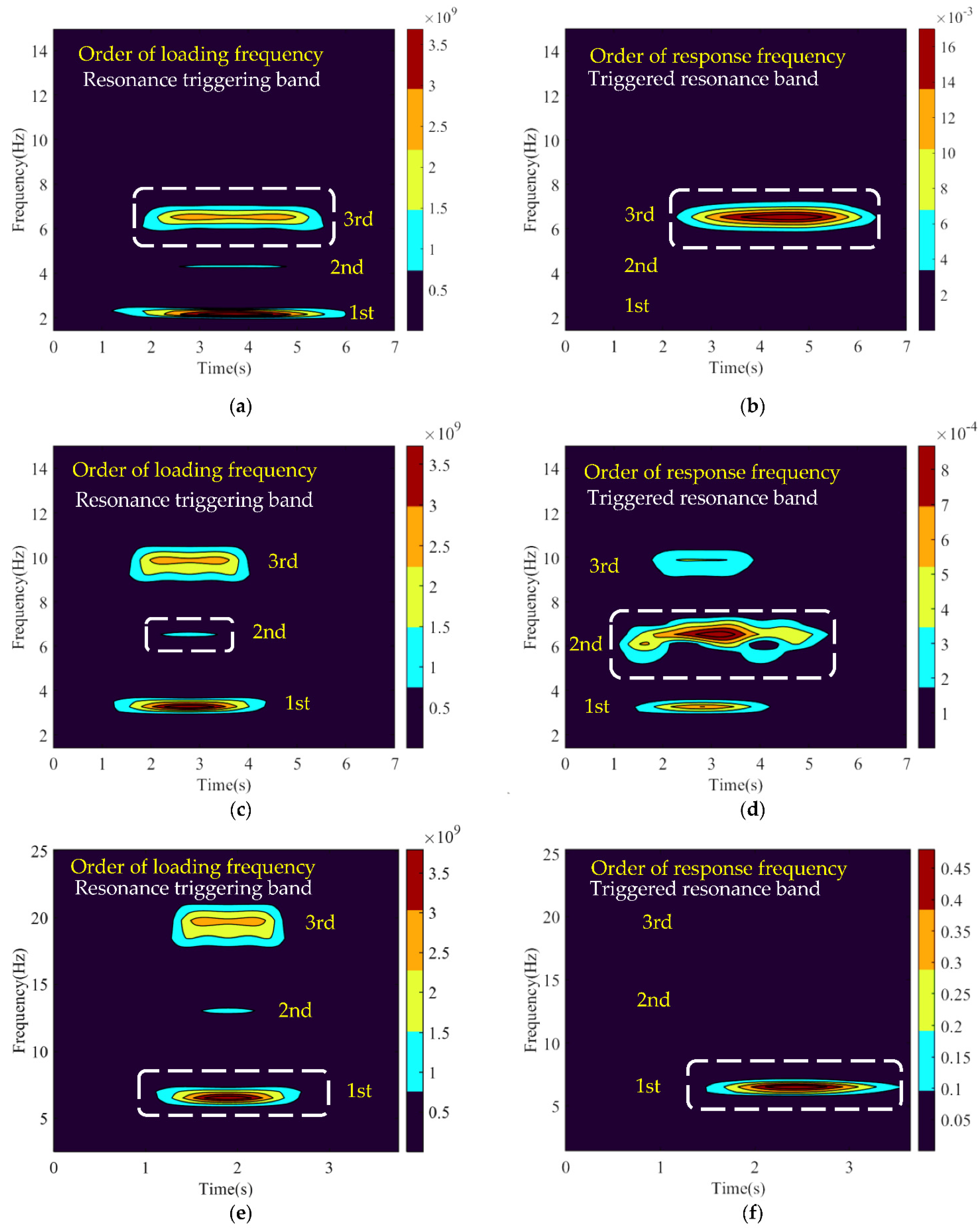
Figure 8.
Scalogram from excitation to vertical vibratory resonantly transitional acceleration response at mid–span bridge: (a) Excitation scalogram at train speed of 175 km/h; (b) Bridge response scalogram at train speed of 175 km/h; (c) Excitation scalogram at train speed of 210 km/h; (d) Bridge response scalogram at train speed of 210 km/h; (e) Excitation scalogram at train speed of 550 km/h; (f) Bridge response scalogram at train speed of 550 km/h; (g) Excitation scalogram at train speed of 680 km/h; (h) Bridge response scalogram at train speed of 680 km/h.
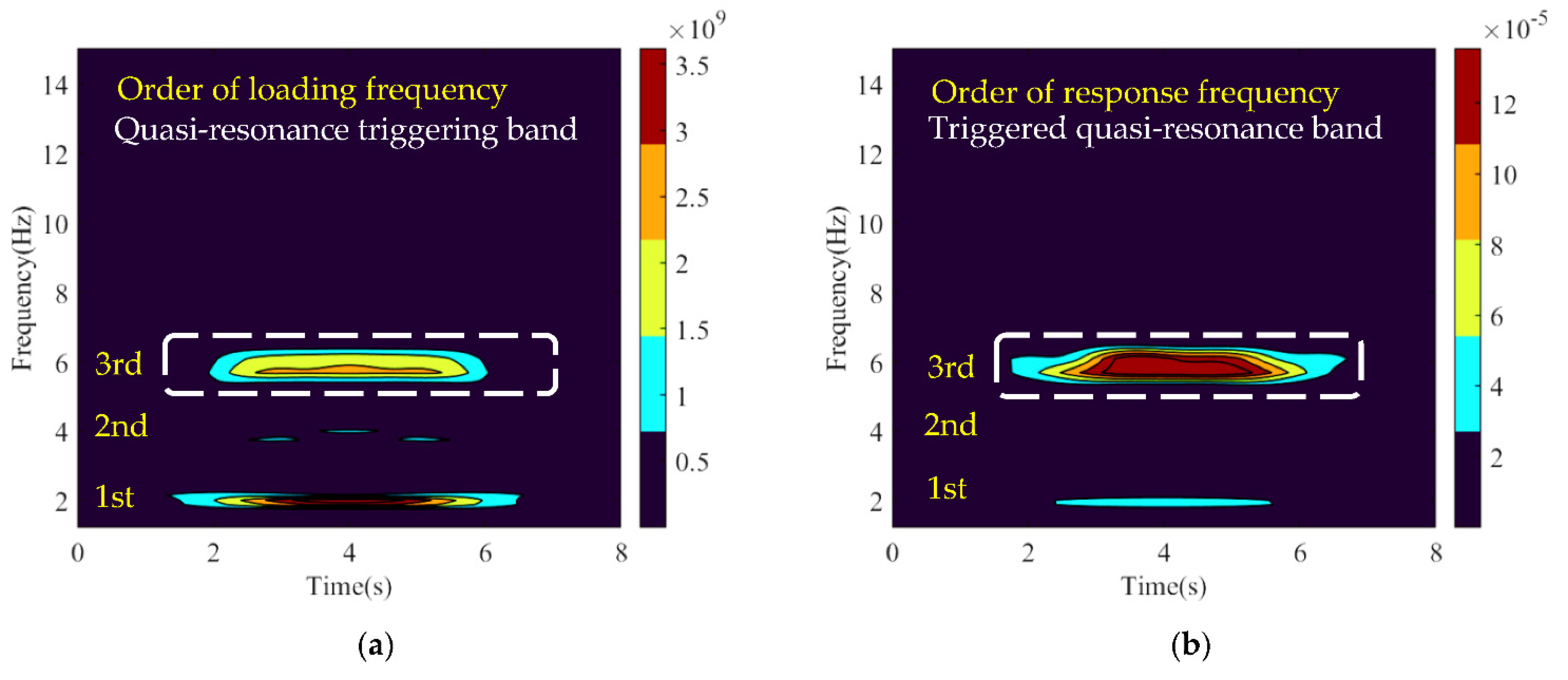

Figure 9.
Scalogram from excitation to vertical vibratory resonant acceleration response at mid–span bridge: (a) Excitation scalogram at train speed of 320 km/h; (b) Bridge response scalogram at train speed of 320 km/h; (c) Excitation scalogram at train speed of 350 km/h; (d) Bridge response scalogram at train speed of 350 km/h; (e) Excitation scalogram at train speed of 400 km/h; (f) Bridge response scalogram at train speed of 400 km/h.
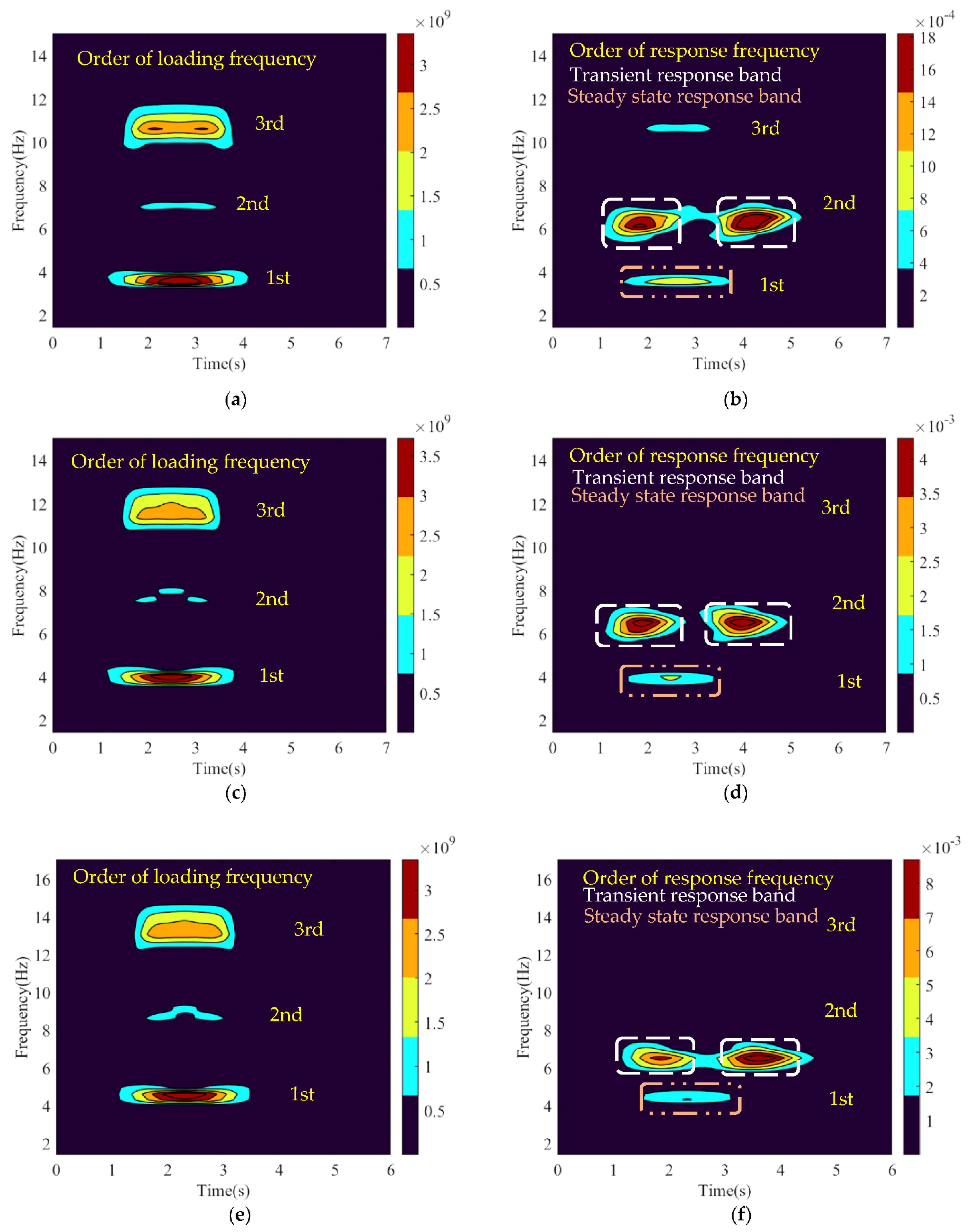
Figure 10.
Scalogram for the track and the car body vertical vibratory resonant acceleration response: (a) First car body response scalogram under nonresonant bridge; (b) First car body response scalogram under resonant bridge; (c) Mid–rail response scalogram under nonresonant bridge; (d) Mid–rail response scalogram under resonant bridge; (e) Mid–sleeper response scalogram under nonresonant bridge; (f) Mid–sleeper response scalogram under resonant bridge.


Table 1.
Parameter values of the train subsystem [21].
Table 1.
Parameter values of the train subsystem [21].
| Train Subsystem Parameter | Value | Unit |
|---|---|---|
| Car body mass mc | 40,000 | kg |
| Bogie mass mb | 3000 | kg |
| Wheel set mass mw | 2000 | kg |
| Car body inertia Ic | 2 × 10⁶ | kg·m2 |
| Bogie inertia IB | 3000 | kg·m2 |
| Primary suspension stiffness k1 | 1 × 10⁶ | N/m |
| Primary suspension damping c1 | 20,000 | N·s/m |
| Secondary suspension stiffness k2 | 2 × 10⁵ | N/m |
| Secondary suspension damping c2 | 10,000 | N·s/m |
| Semi–distance of wheel sets d1 | 1.25 | m |
| Semi–distance of bogies d2 | 8.75 | m |
| Distance of vehicle lv | 25 | m |
| Number of vehicle elements nv | 8 |
Table 2.
Parameter values of track–bridge subsystem [21].
Table 2.
Parameter values of track–bridge subsystem [21].
| Track–Bridge Subsystem Parameter | Value | Unit |
|---|---|---|
| Rail elastic modulus Er | 2.1 × 10¹¹ | Pa |
| Rail inertia Ir | 3.2 × 10⁻⁵ | m4 |
| Rail section area Sr | 7.7 × 10⁻³ | m2 |
| Rail material density ρr | 7850 | kg/m2 |
| Beam element length of rail lre | 3.2 | m |
| Rail length lr | 96 | m |
| Rail damping ratio ξr | 0.01 | |
| Fastener stiffness kf | 1.2 × 10⁸ | N/m |
| Fastener damping cf | 75,000 | N·s/m |
| Fastener space lf | 0.64 | m |
| Sleeper mass ms | 120 | kg |
| Sleeper space ls | 0.64 | m |
| Ballast stiffness ks | 1.8 × 10⁸ | N/m |
| Ballast damping cs | 5.8 × 10⁴ | N·s/m |
| Bridge elastic modulus Eb | 3.5 × 10¹⁰ | Pa |
| Bridge inertia Ib | 22.5 | m4 |
| Bridge section area Sb | 17.5 | m2 |
| Bridge material density ρb | 2500 | kg/m2 |
| Beam element length of bridge lbe | 3.2 | m |
| Bridge length lb | 32 | m |
| Bridge damping ratio ξb | 0.03 |
Table 3.
Parameters of vertical track irregularity.
| Parameters | Value | Unit |
|---|---|---|
| Roughness coefficient Av | 4.032 × 10⁻⁷ | m·rad |
| Cutoff angular wave number nr | 0.0206 | rad/m |
| Cutoff angular wave number nc | 0.8246 | rad/m |
| Lower limit of time tmin | 0 | s |
| Upper limit of time tmax | 30 | s |
| 0.001 | s | |
| Arrival instant on the bridge for the first wheel set t0 | 8lv/V | s |
| Lower limit of angular wave number nmin | π/40 | rad/m |
| Upper limit of angular wave number nmax | 2π | rad/m |
| π/400 | rad/m |
Publisher’s Note: MDPI stays neutral with regard to jurisdictional claims in published maps and institutional affiliations. |
© 2022 by the authors. Licensee MDPI, Basel, Switzerland. This article is an open access article distributed under the terms and conditions of the Creative Commons Attribution (CC BY) license (https://creativecommons.org/licenses/by/4.0/).
Share and Cite
MDPI and ACS Style
Wu, Z.; Zhang, N.; Yao, J.; Poliakov, V. Wavelet Time-Frequency Analysis on Bridge Resonance in Train-Track-Bridge Interactive System. Appl. Sci. 2022, 12, 5929. https://doi.org/10.3390/app12125929
AMA Style
Wu Z, Zhang N, Yao J, Poliakov V. Wavelet Time-Frequency Analysis on Bridge Resonance in Train-Track-Bridge Interactive System. Applied Sciences. 2022; 12(12):5929. https://doi.org/10.3390/app12125929
Chicago/Turabian StyleWu, Zhaozhi, Nan Zhang, Jinbao Yao, and Vladimir Poliakov. 2022. "Wavelet Time-Frequency Analysis on Bridge Resonance in Train-Track-Bridge Interactive System" Applied Sciences 12, no. 12: 5929. https://doi.org/10.3390/app12125929
Note that from the first issue of 2016, this journal uses article numbers instead of page numbers. See further details here.