A Sensor Data-Driven Decision Support System for Liquefied Petroleum Gas Suppliers

Abstract

Currently, efficiency in the supply domain and the ability to make quick and accurate decisions and to assess risk properly play a crucial role. The role of a decision support system (DSS) is to support the decision-making process in the enterprise, and for this, it is yet not enough to have up-to-date data; reliable predictions are necessary. Each application area has its own specificity, and so far, no dedicated DSS for liquefied petroleum gas (LPG) supply has been presented. This study presents a decision support system dedicated to support the LPG supply process from the perspective of gas demand analysis. This perspective includes a short- and medium-term gas demand prediction, as well as the definition and monitoring of key performance indicators. The analysis performed within the system is based exclusively on the collected sensory data; no data from any external enterprise resource planning (ERP) systems are used. Examples of forecasts and KPIs presented in the study show what kind of analysis can be implemented in the proposed system and prove its usefulness. This study, showing the overall workflow and the results for the use cases, which outperform the typical trivial approaches, could be a valuable direction for future works in the field of LPG and other fuel supply.

1. Introduction

With the development of technology, decision support systems (DSSs) are increasingly used in various areas of human activity. They are particularly useful when there is a great volume of available data/information about the considered process, and the data/information itself can come from various sources and assume various forms (e.g., measurement data, text data, graphics, sound, video, etc.). Furthermore, DSSs are useful when there are no simple mechanisms—for data processing and for presenting the most important conclusions resulting from the data—that support the user (e.g., decision-maker) in making decisions about a given process. Depending on the areas and purposes of their application, decision support systems make use of artificial intelligence methods, knowledge engineering, multi-criteria analysis, operational research, and decision theory.

The specificity and requirements of the selected field of application mean that a DSS created for a specific type of industry must take into account and solve unique challenges. To the best of the authors’ knowledge, no DSS for liquefied petroleum gas (LPG) suppliers has been presented so far, which would include a full workflow. Therefore, there is no comprehensive work taking into account the issues of the utilized types of gauges, the quality of the data collected from them, the initial processing of these data, nor the generated predictive models and methods of translating the predictions into everyday decisions and long-term management of the enterprise.

Bearing in mind the above motivation, the goal of this study was to present a decision support system dedicated to LPG suppliers. The system is described by means of a general workflow that can be implemented with various technologies and tools, and such an approach should remain universal despite rapidly changing technologies. Moreover, two main areas of the system application are presented and enriched by use cases. The first area is related to issues of forecasting LPG consumption, and it includes two cases of the system use. The short-term forecast concerns consumption within a time horizon of up to seven days. The medium-term forecast refers to the global (within one storage depository) demand for gas over a three-month horizon. Based on the prognoses, short-term recommendations were built concerning the necessity to provide LPG to certain clients, as well as medium-term recommendations concerning global LPG demand. The second area includes defining, analyzing, and monitoring key performance indicators (KPIs) related to LPG distribution business processes. The KPIs presented in this work monitor the effectiveness of the gas supply process to individual customers. Each use case of the system includes the motivation showing the type of decisions that it can support and the numerical analysis concluded with valuable results

The contribution of this work is the created decision support system. According to the authors’ knowledge, this is the first solution responding to the real needs of LPG suppliers. The subsequent aspects of this contribution refer to the application area of the system created and are listed as follows:

• A new predictive model using attributes related to the weather forecast and historical values of LPG consumption is introduced in this study. The model shows its advantage over the commonly used trivial approaches in both short- and medium-term consumption prediction. In addition to the model, the work introduces a novel method of the gas consumption prediction evaluation and its translation to the delivery recommendation.
• The integration of the enterprise management system with measuring systems is unique. It consists of the mechanism of the on-line generation of KPIs (based solely on measurements data) triggered upon the arrival of a new measurement. Moreover, the classes of performance indicators and key performance indicators defined for the needs of the system are introduced in this work.

The paper is organized as follows. Section 2 presents an overview of previous research related to the presented topics. Section 3 presents the monitoring environment in which the system works. Section 4 outlines a workflow of the introduced system and describes the analytical server. Section 5 presents issues related to the use of predictive models to forecast LPG consumption in the short and medium term. Section 6 outlines the performance indicators defined for the LPG suppliers. The results of the experiments carried out on a real-life data set and the evaluation of the created methods are presented in Section 7. Section 8 concludes the presented work.

2. Related Work

Decision support systems have evolved together with the development of technology [1], and as mentioned in the Introduction, there are several types of DSSs defined in literature [2], namely: data-driven, model-driven, document-driven, communication-driven, and knowledge-driven DSSs. A decision support system can be of one type; however, it can also contain subsystems representing different DSS types.

The characteristic features of data-driven DSSs are the access and processing of time-series, which can be internal company data or external ones [3]. Data that are processed within the system can be stored in various locations starting from a file system, where a query and retrieval functionality is provided to a data warehouse [4,5], where advanced data manipulation methods are available. An appropriate data repository is particularly important for further analysis, inference, and decision support. Thanks to this, it is possible to integrate data from various sources and to clean and prepare them. Such data-driven systems are used for data originating, e.g., from sensors [6,7].

The data stored in a system repository can be processed by means of advanced data analysis methods in order to derive a model assisting in decision-making. Systems where a model plays a central role are called model-driven DSSs [8]. They enable a non-technical user to access a model through a dedicated interface. Additionally, the created model is intended to be applied repeatedly in the same or a similar decision situation. The models utilized in the system can be of various types, e.g., differential equation models, analytical hierarchy process-based models, or forecasting ones.

From the end user’s perspective, what matters is the functionality of the system. Forecasting became crucial for the activity of many companies as prediction-based decision-making can significantly support the company’s operation. As a result, another type of system was distinguished: the forecasting support system (FSS) [9]. A system of this type is characterized by the following two components: a database containing historical time-series and a set of forecasting methods. Another important feature of FSSs is the user’s ability to evaluate forecast quality. Decision support systems where the prediction module played a significant role were designed for a variety of applications, e.g., medicine [10], industry [11], or stock market data [12].

Another very important methodology that can significantly improve company operation is key performance indicators (KPI) [13,14,15]. KPIs are defined by the domain expert [13] and are used to evaluate the efficiency of business processes, monitor their changes, and make decisions about improvements in a company [14,16,17]. KPIs are widely used in supply chain management, as they offer the overall visibility of the supply chain and help to assess the accuracy of a supply/demand plan, as well as execution performance [18].

Considering the domain of the system’s application, a comprehensive review of decision support methods being applied in the upstream oil and gas industry was presented in [19]. This study included a review and classification of over one-hundred works published in the last forty years. In addition, several studies were reported in the field of artificial intelligence application to predict the properties of gas and other petroleum products [20,21].

It can be noticed that the area of gas demand forecast drew significant attention among researchers, yet most of the published research is connected with natural gas demand prediction [22]. Recent works in this field cover prediction at various granularity levels starting from hour [23] to year [24] and from a single building [25] to the whole country [24]. The work by [24] was motivated by the need to improve present and future energy supplies. Additionally, it was highlighted in [23] that predictions are essential for the conclusion of contracts and the development of pipeline infrastructure. On the other hand, in [25], predictions of demand for natural gas were made for the purpose of realizing energy cost savings. The methods used in all the approaches are based on artificial neural networks [23,25] and the hybrid ARIMA-ANFIS model [24]. The resulting prediction models are or can be applied to support decision-making.

Liquefied petroleum gas was considered from the logistics perspective in [26], where the planning and scheduling of LPG deliveries to petrol stations were analyzed. The work by [27] presented the analysis of gas usage for different types of buildings. Gas consumption depends on the building destiny; hence, three classes were identified in this work: housing, housing with high thermal capacity, and industry. Depending on the building class and its characteristics, different models should be applied in order to predict gas consumption. The models utilized in the research were based on auto-correlations of gas usage time-series and different cross-correlations between gas consumption and temperature time-series. Finally, the work by [28] presented a meta-learning-based approach to LPG consumption prediction. This solution uses stacking for the automation of predictive model selection without the definition of the customer classes.

The above-presented review shows that there are works presenting decision support systems of various types and subsystems offering functionality crucial for decision-making. Other works undertake analyses of gas consumption prediction. However, according to the authors’ best knowledge, there is no single study of a decision support system in the field of LPG supply that covers the overall workflow, functionality, and application supported by use cases.

3. LPG Consumption Monitoring and Sensory Data Collection

The background for the created system was the measuring infrastructure collecting sensory data processed by the DSS. LPG is stored in tanks, which are equipped with a measuring system that allows knowing the gas level in the tank. Based on the lowering of the gas level, consumption is calculated. The mechanism of consumption calculation should be insensitive to naturally occurring phenomena, like the instability of the LPG surface or the inaccuracies of the measurement system. Consumers use gas in a volatile phase in most cases. Therefore, the installation can be equipped with a gas meter, which allows more precise measurement of consumption. Furthermore, complementing tank monitoring with a gas meter enables comparative analysis for the values obtained from both measuring instruments. It allows identifying potential irregularities such as: LPG leakage, gas theft, gauge blockage, and gas meter malfunction.

Measurements of the LPG level in the tank can be carried out manually by reading the dial or automatically. There are several methods for monitoring the LPG level in the tank, including: a mechanical system with a float [29,30], a pressure probe, measuring the difference between air pressure and pressure on the bottom of the tank [31], a magnetostrictive level gauge [32], radar technology [33], and IR imaging [34].

The most popular method uses a mechanical system placed inside the tank, which transforms the movement of the float placed on the movable arm into the rotation of the magnetic element in the head located on the top of the tank. Outside the tank, in the head, there is a dial with a pointer indicating the measurement level. The dial and the internal mechanical system are connected magnetically, without physical contact, due to the need to keep the tank leakproof. During the deployment of the automatic meter reading (AMR) system, the dial is replaced by an electronic device containing a Hall effect sensor (reading the direction of the magnetic field lines) and a communication module used for sending measurements wirelessly to the acquisition system. These electronic devices are battery powered and should have a long life time (a min. five years); therefore, the communication model must be energy saving. Particular types of devices use various transmission techniques: Internet of Things protocols (e.g., LoRa [35], Sigfox [36]), local radio transmission using the ISM band (e.g., WM-BUS), or satellite communication (e.g., Hiberband [37]). In the case of local radio transmission, radio frames transmitted by these devices are received by concentrators and then retransmitted to the acquisition system using the cellular network.

The acquisition system platform supports devices operating in many protocols, as well as many types of devices, using a system of plug-ins. Processed data are stored in a database, from which they are read by end user applications. Processed data are also sent to supporting systems such as the system presented in this work. The described monitoring environment and the possibilities of the measurement acquisition system configuration are illustrated in Figure 1.

4. Decision Support System Workflow

The technology enabling the implementation of the DSS created is changing very quickly. Therefore, when presenting the implemented solution, it is worth disregarding the implementation performed and the tools and subsystems used. This work focused on presenting a workflow that, being a universal proposition, can be transferred to selected technological solutions. Figure 2 shows the workflow defined for the created DSS, including the main user roles. The following paragraphs describe the different steps of this workflow.

4.1. Data Pre-Processing

The decision support system is fed with measurements collected by means of the acquisition platform described in Section 3. Each new data example is first directed to the data preprocessing service. At this stage, it is possible, e.g., to eliminate obviously erroneous entries (e.g., data outside of the measurement range) or to reduce the frequency of data recording (by omitting some measurements).

Several transformations applied at this stage are related to the domain in which the DSS created is applied. Figure 3 presents an example plot of LPG level measurements for over a year. It contains several artifacts that have to be addressed at an early stage of the transformations.

One of the fundamental issues for a gas consumption metering and prediction system is the identification of deliveries. Tank refueling is visible on the chart in Figure 3 as a significant and instant increase of the gas level. When calculating gas consumption as the difference in gas level for a given day and the day before, this results in a large negative consumption value that should be set to zero. Typical delivery results in an increase of the gas level by more than 40% of the tank capacity; however, a smaller threshold value (e.g., 10%) should be set.

Negative consumption, but of small value, can also result from the change in gas volume due to temperature changes. This phenomena is visible in Figure 3 between Months 7 and 10 as a very small increase in the gas level. In such a case, the gas consumption value is set to zero, and the gas level preceding the growth is retained in order to be used for further calculation of consumption in the next day. Another problem can be the low sensitivity of the gauge (resulting from its construction utilizing a float). This can cause only significant drops in the gas level in the tank to be registered. In such a case, the same conditions can result in significant gas consumption or a lack of consumption, which leads to an incoherent data set. This can take place especially in the case of small households with low gas consumption. The solution to this problem is averaging the gas consumption values with the use of a sliding window.

Data initially processed are then sent to the data store. This data repository can be designed to store different data structures, and it can consist of different databases. Except measurements collected from LPG tanks, it can store weather data used to generate gas consumption models and to predict the value of gas consumption. The current weather conditions, such as temperature, could be collected by the LPG tanks. However, the temperature sensors mounted on tanks are not reliable because they are vulnerable to sunlight exposure. Additionally, weather data include weather forecasts, which are used to generate gas consumption prediction.

4.2. Data Processing and Presentation

The main process implemented by the system is data processing, as it is related to all other elements of the DSS, and all the DSS functionalities are implemented through processing. The central role in the processing is played by the analytic server presented in Section 4.3. Data delivered to the DSS can be processed in two modes: stream mode is dedicated to processing data immediately upon arrival, in the order of their appearance, whereas batch mode is dedicated to processing data fetched from the data repository according to the assumed schedule.

The processing scheme may be simple—calling a function and returning a single value—or complex, which may be based on the data from a data repository. Complex processing can include various tasks applicable to different phases of data analysis and decision-making. As an example of the initial data processing utilized by further tasks, the recalculation of an aggregate value (e.g., grouped by location and/or time) can be given. In the next step, various machine learning tasks can be mentioned, e.g., calculation of regression coefficients, generating the predictor (if it is expected to be re-trained (adapted) when a specific data packet is delivered), or performing a classification or regression. Finally, the calculation of the KPIs can be defined and scheduled as the last processing task.

Data processing in the DSS created can be executed automatically or can be performed ad hoc. The first case includes predefined and stored processes that are executed according to the adopted schedule. The second approach is based on an analytical environment that supports the design and evaluation of data processing, training, and visualization tasks. Such an environment enables a user to perform, among others, such tasks as searching for dependencies in the data, creating classification and regression models, and assessing and verifying the quality of the created models. The results of such an analysis are stored in the data repository. It can contain ready-to-use processing and analysis schemes (which can be scheduled to be executed on incoming data, both in stream and batch processing mode), the results of the work performed (i.e., the entire environment of the experiment consisting of scripts and reports), and the configuration information defining how to use the obtained results.

The results of processing are used for reporting and visualization. The reporting mechanisms are implemented in the presented system in three ways. The first approach is based on the full functionality of reporting systems providing the possibility of a full report configuration. The second approach is based on reporting interfaces in the form of various types of APIs issued for the client. The last approach can be briefly referred to as reporting in the application and includes the configuration of pre-defined reports from the GUI level and interactive report creation by the operator.

The visualization mechanisms are applied to a series of raw data, aggregates, KPIs, and forecasts. As a result, easily configurable charts, tables, forms, and dashboards are created.

4.3. Analytic Server

The analytic server is the heart of the presented decision support system, playing a central role within processing. Therefore, this module of the created DSS is presented in more detail. The analytic server module is a scalable solution that enables users to conduct advanced data analyses and to build intelligent applications based on these analyses. The server gives access to ready-to-use, predefined analysis methods and has mechanisms that allow for launching implemented procedures in the Python and R languages.

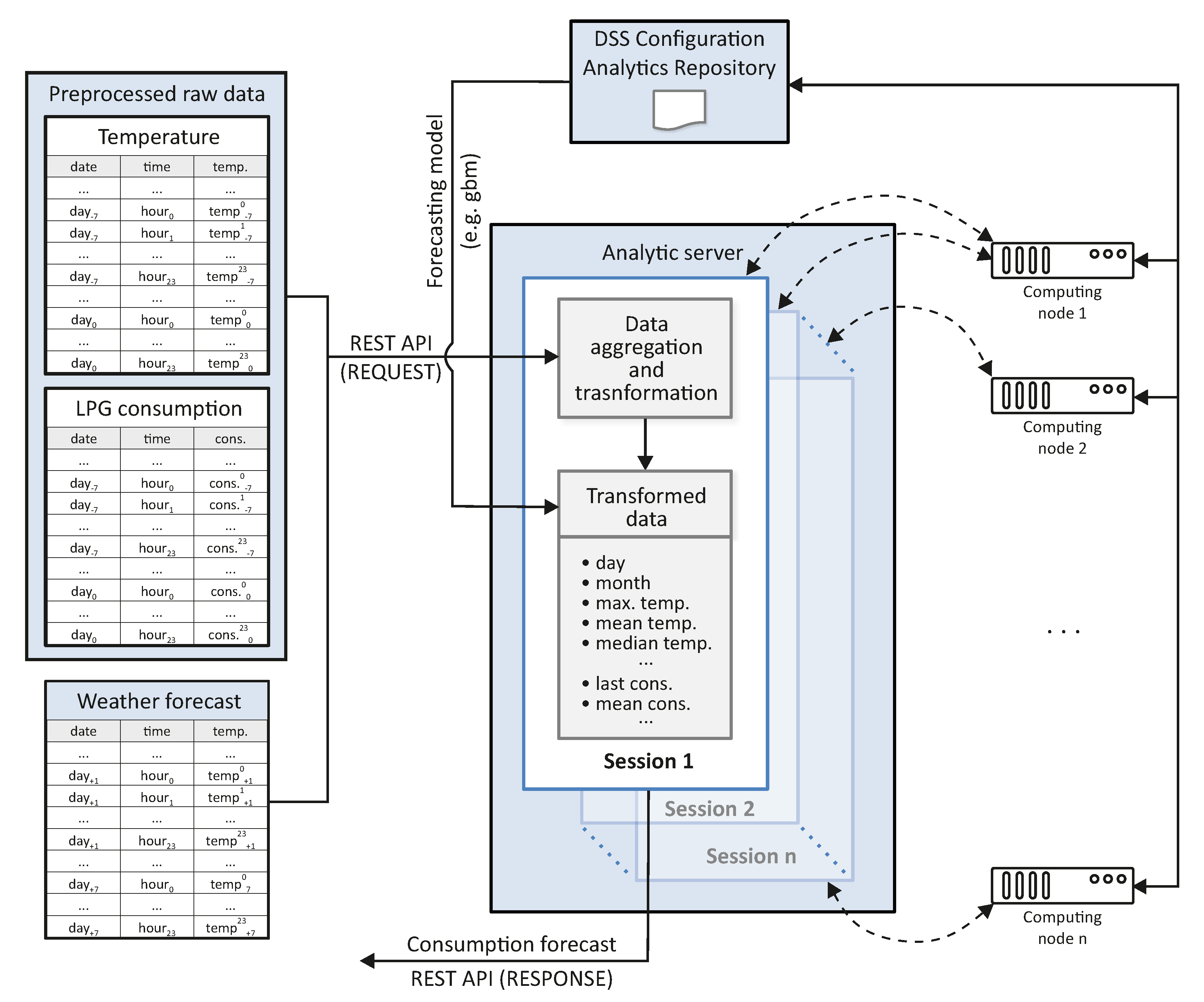
The analytic server may be launched both on a single server and on a cluster. Therefore, the solution can be scaled to a problem of any dimension. Figure 4 illustrates the analytic server operation when the task of LPG consumption prediction is carried out.

The analytic server is responsible for providing the interface accessible to external applications, receiving requests from clients, and delegating tasks. The tasks commissioned by external applications are carried out on computing nodes by means of the so-called computing engines, which make it possible to execute the Python and R codes. The database stores indispensable configuration data, such as information about services available on the server, users, and their privileges.

The analytic server provides access to a number of services, which allow the client application to manage the server and its assets. Depending on the privileges granted to the logged-in user, the client has access to the following functions:

• management of users and their privileges,
• management of computing nodes,
• using the server in the session mode (from the opening to the closing of the session; online, the client uses the terminal of the chosen computing engine, which allows executing one’s own Python or R code),
• management of computing services.

The computing node is a target device on which client-commissioned tasks are launched by means of services accessible on the analytic server or during the work within a session. The node manager application is set off on the node, and the analytic server communicates with that application. The task of the manager is to execute and manage the instances of the Python and R computing engines.

4.4. Users of the System

There are three types of DSS users identified in Figure 2: data scientist, data analyst and services.

The data scientist is an expert in data science who performs statistical analysis and data dependency studies and who builds the data processing models. The data scientist operates in the presented above analytical environment. Besides, this user performs the configuration of reports and dashboards. Finally, the data scientist completes the tasks ordered by another user—the data analyst. Such tasks can include, e.g., building the up-to-date predictive model generating LPG demand prognoses.

Data analysts are domain experts. They analyze and supervise business processes performing the daily analysis of business KPIs, the analysis of reports’ data, and research on identified anomalies. Data analysts use defined procedures in an environment that consists of reporting and visualization tools, as well as analytic methods developed by the data scientist. The data analyst can commission the data scientist to implement the new visualization functionalities, new KPI indicators, or analytical tasks that are not available in their analytical environment.

Service users are end users who measure and verify the service level agreement fulfillment. Two types of users belonging to this group can be indicated. The first type of service users operates on dashboards and monitors and plans daily deliveries. These delivery operators decide where and when the tankers should be directed and what the route of each tanker should be. The other type of service users makes business decisions on the basis of KPI values and alerts about high risk events and predicted total gas demand. Managers of this type operate with a medium- and long-term perspective, and their task is to prepare an appropriate stock and long-term optimization of the supply process.

Summarizing the presented user types: the data scientist user works on the DSS site developing its analytical functionality; the data analyst user is on the edge of the system and its application domain; while the service users utilize the DSS in daily operation and make strategic business decisions.

5. Consumption Forecasts

Having reliable forecasts allows enterprises to gain a significant advantage in business. Therefore, currently, forecasting has become an extremely important service that can bring measurable benefits to the supplier. The LPG consumption forecast in this work was considered from two different perspectives—short- and medium-term.

5.1. Short-Term LPG Consumption Prediction

Short-term LPG consumption prediction supports the every day operation of the LPG supplier visualizing the predicted gas level in every customer’s tank. Therefore, it helps to decide where and when to deliver the gas, and it is performed for each tank in a 1–7 day horizon.

It was assumed in this work that the analysis is performed on the tanks that are equipped with meters that can communicate with the supplier IT infrastructure sending gas level measurements. Due to regular sensor readings reporting the LPG level, it is easy to correctly react to and refuel the tank when the gas is scarce at a given location. However, from the economical point of view, sending a transport vehicle that refuels the tank as rarely as possible is the most profitable. This means that sending a tanker truck to a client location where there is still a sufficient fuel supply can be classified as mismanagement in most cases. In order to safely balance fuel availability, thorough predictions are required.

Another motivation for short-term LPG consumption prediction is a situation when the number of transport vehicles necessary on a given day exceeds the capacity available for a supplier. It is then required to minimize the risk of delayed delivery to selected clients. Again, the evaluation of such a risk should be based on thorough predictions.

Referring to the workflow presented in Section 4, the analysis starts by collecting the raw data for the decision support system. In the case of the short-term LPG consumption prediction, the raw data consist of:

• measurements collected by telemetry such as time and the gas level in the tank,
• measurements collected by meteorological stations such as time and temperature,
• weather forecasts consisting of time and predicted temperature.

Raw data are preprocessed and stored in a data repository. These data are then retrieved by a data scientist user who has a specific business task—creating predictive models. Therefore, the data scientist has to properly prepare data for the model, e.g., selecting attributes and generating derived variables. Next, the created models are tested and selected depending on their quality. As a result, the selected predictive model and a feature vector derived for this model are stored in the data repository.

In the next step, a series of calculations are triggered according to the schedule defined. Therefore, forecasts or the recommendation algorithm can be invoked. This process is carried out in the shape of a pipe, where data exchange is carried out through the data repository. On the basis of the resulting predictions, the recommendation and visualization (see Section 5.1.2) are presented.

5.1.1. Short-Term Prediction Models

LPG consumers can be of different types and can include, e.g., a single-family house, a bakery, a primary school, a farm, or a factory. Their gas consumption can be, therefore, temperature dependent, constant, seasonal, or of a different type. Figure 5 presents two examples of consumption plotted in time, where the months of the year are marked as x-axis labels and the fraction of the tank’s capacity is marked on the y-axis as consumption. Temperature-dependent consumption (Figure 5b) is characterized by higher values during winter months and lower values during summer. In the case of the other plot (Figure 5a), no dependency on temperature nor other seasonal changes can be recognized.

The most typical and unambiguous is the temperature-dependent characteristic of LPG consumption, which is presented in Figure 5b. In such a case, LPG consumption can depend on minimal and maximal daily temperature values and the aggregated values, e.g., mean or median temperature. An example of the dependence of consumption on median daily temperature is visualized in Figure 6a). Such a dependency can be modeled by some kind of regression or a combination of linear models (see Figure 6), e.g., generated in the form of a regression tree.

Having in mind that customer consumption characteristics may be of different types (not only purely temperature based), the proposed model may be extended to other features, e.g., such as the number of the day of the week or the number of the month.

5.1.2. Application of Short-Term Prediction Results

The result of the forecasting model operation is a predicted LPG consumption for a given tank. The predictions are then used to calculate the predicted gas level in a tank. Information on the action recommended for a given gas level are presented to a system operator and support their decisions. Two types of evaluation are introduced in the proposed system.

The first type of evaluation supports the data scientist in deciding whether the quality of a given predictive model is acceptable, and the model can be implemented in the system operation. The performance of the prediction model can be evaluated by means of typical quality measures used in regression applications, e.g., root mean squared error (RMSE) or mean absolute error (MAE). Additionally, relative versions of these measures can be used (rRMSE and rMAE) in order to verify if the proposed models offer better results compared to the trivial approaches.

The second type of evaluation supports the end user in decisions where risk evaluation is required (e.g., when the number of transport vehicles necessary on a given day exceeds the capacity available for a supplier). In such an approach, valuable information is introduced by an error range calculated for each prediction horizon on the basis of past predictions. The error range can assume the form of an error distribution or a confidence interval. Therefore, one of the approaches involves applying a boxplot representing historical error values on a predicted consumption plot. Another method is to plot the predicted LPG level within the confidence intervals calculated for a chosen confidence level. In both cases, the final user receives a visualization of the predicted gas level and a clearly plotted range that can be taken into consideration if needed.

Examples of the boxplot visualization are presented in Figure 7. The plots were created for a single prediction in a seven day horizon. The gas level is reported as a percentage of the tank capacity. The predicted gas level is plotted as dots connected by a solid line for trend visualization. Each predicted value (a dot) is accompanied by the error range calculated on the basis of the predictions that were performed in a time range of 50 days preceding the given prediction. A dotted line at the gas level value equal to 0.2 indicates the level for which delivery should be made immediately.

The predicted gas level in a tank and the possible error range are the pieces of information that support the final decision made by the user controlling the delivery of gas to customers. There are three action recommendations: must go, can go and do not go.

The algorithm supporting a logistics specialist in planning deliveries to individual customers is based on current and forecasted gas levels in customer tanks. The forecasted level is based on the gas consumption forecast. Each tank has defined fuel level thresholds denoted as: $HH$—very high fuel level; H—high fuel level (the tank should be filled slightly above this value; L—low fuel level (delivery should be made immediately after the fuel level drops below L; $LL$—too low fuel level; installation may be damaged). The recommendation algorithm supporting a logistics specialist in the planning of deliveries is parameterized, with the main algorithm parameter reflecting the level of risk accepted by the logistics specialist. There are two aspects to this risk. The first one corresponds to the situation when the delivery was sent too late and the tanker did not arrive at a customer who exceeded a drop below level L. The second aspect corresponds to the situation when the delivery was sent too early and a tanker arrived at a customer for whom the gas level will be maintained above level L in the next few days, and therefore, the delivery would not be optimal in terms of the volume of gas to be poured into the tank. An ideal situation would be to deliver gas at the L level (or slightly lower) and filling the tank up to H (or slightly above H).

The gas consumption forecast of each predictor can be enriched with the ranges calculated in relation to the errors of the given forecasting model and their distribution calculated on historical data (Figure 7). In order to formally define how the ranges influence the recommendations for logistic specialists, let us determine by f the predicted value of gas consumption in the given forecast horizon, and additionally, let us characterize the prediction error distribution on the last n examples by the following values: $Q_1$—first quartile, $Q_2$—median, $Q_3$—third quartile, $IQR$—interquartile range ($Q_1$ to $Q_3$), $V_1=Q_1-1.5\ast IQR$, and $V_3=Q_3+1.5\ast IQR$, where typically, $Q_2$ is a value around zero, whereas $V_1$ and $Q_1$ are values below zero. The location in a given forecast horizon is indicated as:

• must go if the forecast for the tank’s fuel level resulting from the range $r_Q$ (where $r_Q=f+Q_1$) would cause the fuel level to drop below the value of L,
• can go if the forecast for the tank’s fuel level resulting from the range $r_Q$ would not cause the fuel level to drop below L, whereas the level resulting from the range $r_V$ (where $r_V=f+V_1$) consumption forecast would already cause such a drop,
• do not go if the forecast for the tank’s fuel level resulting from the range $r_V$ would not cause the fuel level to drop below the value of L.

Additionally, in each group of tanks, they may be ordered according to the proximity of the predicted corrected fuel level to the group boundary {$r_Q$, $r_V$}.

The values $Q_1$ and $V_1$ would typically illustrate the error distribution on a boxplot. When they are combined with the predicted LPG level f, the boxplot characterized by the values $r_Q$ and $r_V$ is received, which is presented in Figure 7. Considering the seventh day recommendation in Figure 7, the must go recommendation would be issued for Case (a), and the can go recommendation would be issued for Case (b).

5.2. Medium-Term LPG Consumption Prediction

Medium-term prediction supports the supplier’s strategic planning at the company level from a longer perspective, e.g., three months or half a year. When setting the perspective at the company level, what matters is not the gas consumption on a given day per single customer, but rather the predicted total gas capacity that will be consumed within a given period of time. Thanks to this information, it is possible to anticipate and mitigate, e.g., a situation when the gas demand for a given period would exceed the available reserves. This allows for planning increased purchases in advance and for preparing appropriate agreements with partners regarding the provision of storage space and gas-transporting rolling stock.

Prediction at the delivery area level or even that of the whole company can be broken down into predictive tasks defined for each tank similarly to the short-term prediction problem. However, while short-term prediction models can be based on recent trends and local features, e.g., temperature forecast or gas consumption in the last days, medium-term prediction models have to be based on more general attributes.

In the case of a medium-term approach, where the prediction horizon is at least three months, it is not possible to retrieve the temperature values that are the basis for prediction from a weather forecast. However, having the temperature measurements from the last few years, it is possible to calculate climate-like temperature as a mean of the available values of each day of a year. This way, the generated predictor models the consumption dependency on a general climate information. Such an approach may result in large error values for short-term prediction, when current temperature values can significantly differ from the long-term average. However, a total relative error within a longer period may be reasonable.

Referring to the workflow presented in Section 4, similar to the short-term LPG consumption prediction, the medium-term LPG consumption prediction is generated within the process in which the data transformation and modeling are performed.

6. Key Performance Indicators

Key performance indicators (KPI) are one of the simpler tools that support the management of almost every area of an organization’s functioning. The indicators can be used to assess business processes in companies of different trades. The biggest challenge related to business processes’ management through monitoring KPI values is to define proper measures that really illustrate the most important parameters of the process.

People involved in the performance or supervision of a given process are usually able to define from several to even several dozen different indicators, all of which describe the monitored process in a certain context. The issue is how to select crucial indicators for each group of users. While defining the indicators [13], the pyramid rule applies. The majority of indicators refer to the so-called shop floor where technical and maintenance personnel analyze indicators related to the current quality, failure frequency, and efficiency of performed processes. Successive indicators are defined for lower and higher management. The final group of indicators is defined for managers. The higher the position in the management hierarchy, the higher the frequency at which technical indicators are replaced with economic and organizational ones. In addition, according to the applied terminology, the indicators for higher management and managers are referred to as key indicators (usually, there are only several of them), while those for technical and lower managers are called performance indicators (PIs). It is possible to define several dozen performance indicators as particular groups of personnel or department managers are only responsible for the values of indicators associated directly with their duties. Part of the KPIs related to measuring the efficiency of technical resource use are defined as overall equipment effectiveness measures [16].

Machine learning methods can be used to investigate the impact of particular process indicating parameters on the PI and KPI values. In particular, it is possible to define a KPI without quoting its analytical formula, treating the parameter only as a certain value that can be calculated (e.g., average cost of supplying 100 L of liquefied petroleum gas to an individual user), while machine learning methods can be used to check which of the monitored process parameters (apart from the obvious ones, such as the number of kilometers covered) impact the value of the indicator. The data analysis method applied in such investigations should generate a data model that can be interpreted by humans (e.g., a tree or set of rules). Such attempts have been described in the literature, e.g., in [38,39].

While developing a decision support system for LPG distributors, over 100 performance indicators were defined. The indicators allowed monitoring the areas of secondary bulk distribution or customer tanks. Within the secondary bulk distribution, the following indicators were defined:

• delivery indicators that analyze the volume of gas supplied by a set number of tankers to a set number of clients within a set period of time,
• capacity indicators that analyze the efficiency of tanker use from the point of view of the volume of supplied gas in relation to the tankers’ capacity,
• trips indicators that analyze the efficiency of tanker use from the point of view of the number of kilometers covered and the number of performed deliveries,
• costs indicators that analyze the costs of the deliveries and the tankers’ maintenance in terms of the supplied volume of LPG.

The following indicators were defined within the customer tank area:

• drop size indicators that illustrate the volume of gas supplied to the tank,
• LPG level indicators that point to the level of gas in the tank, in particular the states below and above the warning values and the lack of gas in the tank,
• consumption profile and consumption forecast indicators that describe the (real and predicted) volume of gas used.

The indicator values were analyzed for a period of time, client, group of clients, location, and type of service.

Table 1. KPI examples for the customer tank area.

Indicator Name	Units	Description
Total Residual Space	L	Unused spaced in the tank directly after the delivery. The lower the value is, the better [0, tank capacity).
Relative Drop Size	%	The volume of delivery expressed as the quotient of the supplied gas to the tank’s capacity (expressed in %). For a bigger number of deliveries, a bigger number of tanks, etc., an average value is calculated that can serve as a reference value for single tanks. The higher the value is, the better [0, 100].
LL Level		The number of registered gas levels below the L threshold value. The lower the value is in the range [0, inf), the better, as the gas level in a tank should not drop below level L.
Unit Trip Load Efficiency	%	Delivery efficiency expressed as the quotient of the number of actually performed deliveries to the theoretical number of deliveries assuming that each performed delivery has been fulfilled in an ideal manner (i.e., L is the level of gas in the tank(s) at the time of the delivery, while H denotes the level of gas in the tank after the delivery, which should not be exceeded). The value of the indicator is decreased by 1 in order to indicate the best performance by a 0 value, and it is expressed in % as a value from the range [0, inf). This KPI can also be calculated for each tank separately and compared with the average value for the bigger number of tanks.
Illegal Loads		Calculated as the difference between the number of deliveries to the tank identified on the basis of telemetric data and the number of deliveries to the tank according to the distributor’s data. The lower the value is, the better [0, in).
Customer Consumption	L	Volume of gas used.
Low/High Level Time	Min	Time exceeding the level of gas below (above) values LL, L, H, and HH. The indicator values can be calculated for each tank separately. The lower the value is, the better [0, inf).

features seven KPI examples for the customer tank area.

Finally, it is worth completing the presented KPI description with the perspective of the system that was created. The values of the KPIs are calculated by means of the analytic server once a day and stored in the data repository as two tables, of which one stores the values of the PIs, the other the KPIs. The tables have the form of columns as the number of indicators is predefined. Adding new indicators results in a new table in the the data repository. The basic period for which a KPI is calculated is one day; other periods are one week, two weeks, one month, one quarter, and one year. The database stores all aggregated values. After each of these aggregation periods, the new values of the indicators are calculated automatically, which makes the visualization and analysis of indicator values very fast. KPI visualization enables various analyses. KPI values can be analyzed taking into consideration different perspectives (dimensions) such as a fixed period of time, client, group of clients, location, and type of service. The indicator values can be compared in the successive periods of time. Therefore, the target line or the value range in which the KPI should fit can be defined, and the trend line enabling prediction of future KPI values can be adjusted.

7. Case Study

Section 5 and Section 6 presented the advanced analytical solutions that can support, within the workflow presented in Section 4, the decisions of the system end users. In this section, the examples of the application of these solutions are presented to show the value of individual methods and analytical approaches that are worth implementing in the future in systems of this type.

The presented DSS is a fragment of a larger conglomerate of systems. Therefore, the results generated by the created system are processed further, in combination with other data held by the LPG supplier, such as information on the routes of LPG delivery vehicles; they constitute a decision value for the end users (service users defined in Section 4.4). Figure 8 presents a fragment of the operator’s application window. It contains decisions on the deliveries to specific customers and a map on which tanker routs are planned.

However, in the framework of this study, available real-life sensory data were used. Therefore, the experiments that were carried out could not cover the operation of all systems used by the LPG supplier. The analysis focused on the methods created showing their advantages over commonly used approaches.

7.1. Short-Term Prediction Example

The exemplary short-term prediction presented below was performed on 19 tanks. A data set spanning between 849 and 1274 days of measurements was collected for each tank. The values recorded for the tank consisted of a gas level measured daily and an outside temperature collected hourly from a weather server. Daily LPG consumption was calculated on the basis of the gas level in a tank. The task was to predict gas consumption for each tank in a seven day horizon. Gas consumption in this task was calculated in cubic meters. Prediction was performed for each day separately, which required the creation of separate models predicting gas consumption on Days 1, 2, …, 7. Additionally, an assumption was made that a model should be applied as quickly as possible, and it can be re-trained after a selected period of time.

In order to create a prediction model, the data sets collected from different tanks were analyzed, and two groups of customers were identified. The first group, which can be named temperature dependent, can be represented by the customer whose consumption is characterized in Figure 6a, while the second group, which can be named temperature independent, can be represented by the customer whose consumption is characterized in Figure 6b. The characteristics of both types of customers using the Pearson correlation and determination coefficients are presented in

Table 2. The dependence of LPG consumption on outside temperature values expressed by means of the Pearson correlation coefficient (PCC) and the determination coefficient (R${}^2$).

Tank	Temperature Dependency	PCC	R${}^2$
1	dependent	−0.679	0.461
2	dependent	−0.651	0.424
3	dependent	−0.474	0.225
4	dependent	−0.612	0.374
5	dependent	−0.490	0.240
6	dependent	−0.717	0.514
7	dependent	−0.758	0.575
8	dependent	−0.571	0.326
9	dependent	−0.809	0.655
10	independent	−0.259	0.067
11	independent	−0.279	0.078
12	independent	−0.413	0.171
13	independent	0.039	0.001
14	independent	−0.128	0.016
15	independent	−0.261	0.068
16	independent	0.102	0.010
17	independent	−0.207	0.043
18	independent	−0.094	0.009
19	independent	−0.238	0.057

. Due to the clear difference between customers, the use of a temperature-only model (like the linear regression or regression tree mentioned in the previous section) is not recommended. Therefore, the more general approach was introduced and based on one of the leading models, which was the gradient boosting model, and its implementation is included in the gradient boosting machines (gbm) R package [40,41].

The size of the generated gradient boosting model was limited to 100 decision trees. The other parameters of the method were set to default values. The model required training data of at least 50 days of measurements and was re-trained each month. Therefore, if the first two months failed to provide enough data to generate the first model, then it was generated only after three months. Moreover, this approach meant that every month, a new, re-trained model was applied and evaluated on another portion of data.

In order to make the model general and applicable regardless of the temperature-based customer type, the following attributes describing each day and combining the information on both the outside temperature and the consumption in recent days were derived:

• mean temperature value within a day,
• median temperature value within a day,
• range of temperature values within a day,
• maximal temperature value within a day,
• minimal temperature value within a day,
• change in the temperature maximal, minimal, and mean value between the current day and one to ten days back,
• mean gas consumption within 3, 5, and 7 recent days,
• change in gas consumption within 3 and 5 days and 3 and 7 days,
• change in gas consumption between the current day and one to ten days back.

Due to the fact that the created model used outside temperature to derive several attributes, it is referred to as temperature based.

Other approaches used in the experiments can be treated as baseline solutions that are typically available for the LPG suppliers and support the daily management of gas supplies to customers. These methods provide the reference level for the temperature-based approach. Therefore, comparing them with the predictive model would allow justifying the suitability of using solutions based on machine learning.

The baseline approaches were based on consumption values only and are collectively named as trivial because they calculated the predicted value as one of the following:

• the last registered consumption value,
• the mean consumption value from the last seven days,
• the median consumption value from the last seven days.

These approaches are referred to as trivial last, mean, and median, respectively. They can be applied just after one or seven days (respectively) of measurements, and they were re-calculated after each day.

The quality of the applied models is expressed by means of the root mean squared error (RMSE):

$$E_{RMSE}=\sqrt{\frac{1}{T}{\Sigma }_{t=1}^T({\widehat{y}}_t-y_t{)}^2},$$

(1)

where T is the time of analysis in days corresponding to the number of examples, ${\widehat{y}}_t$ is a predicted consumption value on day t, and $y_t$ is an actual consumption value on day t.

The results obtained for each model are presented in

Table A1. Short-term prediction error (RMSE) of the temperature-based model—application to 19 tanks, 7-day prediction horizon.

	1	2	3	4	5	6	7
1	0.026	0.026	0.026	0.026	0.026	0.026	0.026
2	0.194	0.177	0.180	0.181	0.211	0.213	0.214
3	0.085	0.081	0.093	0.092	0.099	0.103	0.096
4	0.107	0.109	0.107	0.125	0.124	0.129	0.133
5	0.078	0.079	0.078	0.079	0.081	0.079	0.079
6	0.032	0.033	0.034	0.034	0.034	0.035	0.035
7	0.040	0.041	0.041	0.041	0.041	0.042	0.041
8	0.026	0.029	0.031	0.029	0.030	0.031	0.031
9	0.052	0.051	0.051	0.053	0.050	0.047	0.043
10	0.036	0.038	0.039	0.040	0.041	0.041	0.040
11	0.029	0.031	0.031	0.031	0.031	0.032	0.032
12	0.167	0.178	0.177	0.180	0.182	0.180	0.182
13	0.018	0.018	0.018	0.018	0.019	0.018	0.018
14	0.190	0.198	0.200	0.197	0.199	0.203	0.197
15	0.031	0.033	0.033	0.034	0.035	0.036	0.037
16	0.022	0.022	0.022	0.023	0.022	0.022	0.022
17	0.092	0.093	0.096	0.075	0.079	0.075	0.077
18	0.259	0.263	0.268	0.260	0.265	0.265	0.262
19	0.049	0.050	0.051	0.052	0.051	0.052	0.051

,

Table A2. Short-term prediction error (RMSE) of the trivial last model—application to 19 tanks, 7-day prediction horizon.

	1	2	3	4	5	6	7
1	0.158	0.158	0.158	0.125	0.158	0.158	0.158
2	0.317	0.290	0.300	0.305	0.348	0.349	0.339
3	0.255	0.273	0.293	0.290	0.275	0.302	0.281
4	0.512	0.487	0.467	0.516	0.365	0.518	0.492
5	0.104	0.105	0.105	0.107	0.108	0.109	0.111
6	0.045	0.044	0.045	0.047	0.048	0.047	0.048
7	0.052	0.062	0.061	0.063	0.062	0.058	0.050
8	0.053	0.061	0.062	0.063	0.062	0.063	0.062
9	0.121	0.120	0.120	0.121	0.120	0.121	0.119
10	0.047	0.047	0.051	0.052	0.054	0.057	0.057
11	0.050	0.050	0.051	0.054	0.053	0.054	0.054
12	0.213	0.245	0.237	0.245	0.258	0.250	0.236
13	0.033	0.031	0.032	0.028	0.031	0.031	0.030
14	0.268	0.291	0.304	0.308	0.299	0.291	0.289
15	0.044	0.049	0.052	0.053	0.052	0.052	0.053
16	0.032	0.031	0.032	0.031	0.032	0.030	0.030
17	0.217	0.222	0.210	0.200	0.200	0.198	0.198
18	0.357	0.381	0.381	0.377	0.377	0.364	0.343
19	0.065	0.077	0.078	0.077	0.080	0.071	0.063

,

Table A3. Short-term prediction error (RMSE) of the trivial mean model—application to 19 tanks, 7-day prediction horizon.

	1	2	3	4	5	6	7
1	0.116	0.116	0.116	0.116	0.122	0.122	0.122
2	0.259	0.210	0.215	0.217	0.272	0.274	0.274
3	0.205	0.190	0.209	0.203	0.212	0.234	0.217
4	0.358	0.359	0.365	0.359	0.359	0.385	0.385
5	0.080	0.082	0.083	0.085	0.086	0.087	0.086
6	0.035	0.035	0.036	0.037	0.037	0.037	0.038
7	0.044	0.045	0.045	0.046	0.046	0.047	0.047
8	0.040	0.042	0.044	0.046	0.046	0.048	0.048
9	0.091	0.091	0.091	0.090	0.090	0.090	0.090
10	0.041	0.042	0.044	0.045	0.047	0.047	0.048
11	0.040	0.041	0.042	0.044	0.045	0.046	0.046
12	0.183	0.193	0.197	0.201	0.203	0.203	0.205
13	0.023	0.022	0.022	0.022	0.023	0.023	0.023
14	0.221	0.225	0.228	0.228	0.229	0.230	0.229
15	0.039	0.041	0.042	0.042	0.042	0.043	0.044
16	0.023	0.023	0.023	0.023	0.023	0.023	0.024
17	0.166	0.167	0.167	0.136	0.135	0.123	0.122
18	0.281	0.281	0.287	0.282	0.281	0.280	0.280
19	0.055	0.057	0.057	0.057	0.058	0.057	0.057

and

Table A4. Short-term prediction error (RMSE) of the trivial median model—application to 19 tanks, 7-day prediction horizon.

	1	2	3	4	5	6	7
1	0.112	0.112	0.112	0.112	0.112	0.112	0.112
2	0.259	0.207	0.212	0.214	0.271	0.268	0.268
3	0.200	0.177	0.201	0.194	0.211	0.232	0.209
4	0.363	0.364	0.365	0.366	0.366	0.367	0.367
5	0.081	0.082	0.084	0.085	0.086	0.086	0.086
6	0.035	0.036	0.037	0.037	0.038	0.038	0.038
7	0.047	0.049	0.049	0.049	0.049	0.050	0.050
8	0.038	0.041	0.042	0.044	0.045	0.045	0.046
9	0.086	0.086	0.086	0.087	0.086	0.086	0.085
10	0.041	0.043	0.045	0.046	0.047	0.048	0.049
11	0.042	0.043	0.044	0.045	0.046	0.047	0.048
12	0.187	0.196	0.200	0.205	0.207	0.208	0.210
13	0.024	0.024	0.024	0.024	0.024	0.024	0.024
14	0.231	0.235	0.234	0.232	0.235	0.238	0.240
15	0.042	0.043	0.044	0.044	0.044	0.045	0.046
16	0.024	0.024	0.024	0.024	0.024	0.024	0.024
17	0.157	0.159	0.159	0.122	0.121	0.122	0.121
18	0.290	0.285	0.292	0.287	0.284	0.286	0.284
19	0.059	0.060	0.062	0.062	0.063	0.061	0.062

in the Appendix A, whereas the summary containing aggregations of the calculated error values is presented in

Table 3. Short-term prediction error (RMSE) of gas consumption (m${}^3$)—analysis of 19 tanks, 7-day prediction horizon.

	Min.	1st Qu.	Median	Mean	3rd Qu.	Max.
Temperature based	0.018	0.031	0.050	0.083	0.108	0.267
Trivial last	0.028	0.052	0.107	0.159	0.268	0.518
Mean	0.022	0.043	0.085	0.123	0.205	0.385
Median	0.024	0.044	0.085	0.122	0.207	0.367

.

The results presented in Table 3 show that the performance of the proposed temperature-based model was better than all the trivial approaches. Looking at the source error values, it can be seen that none of the error values presented in Table A2, Table A3 and Table A4 and characterizing trivial models were lower than the respective values in Table A1. In addition, among the trivial models, the mean and median were better then the trivial last approach, whereas there was no clear difference between the mean and median methods.

Analyzing the results from the perspective of the models generated for different prediction horizon values, it can be seen that the error values increased slightly for most tanks with the increasing prediction horizon, apart from the model type.

7.2. Medium-Term Prediction Example

As was stated in Section 5, the short-term prediction model results can be aggregated to perform the forecasts of total gas capacity in a given (longer) period. Therefore, in this experiment, the task was defined as the prediction of the total demand for gas in a three-month period for a distribution station serving 749 customers. The measurements creating the data set were collected for a period from 1 January 2016 to 31 October 2018. They consisted of the daily gas level values for each customer location and hourly values of outside temperature measured at the selected weather station representative of the whole region.

The proposed approach predicted daily LPG consumption for each tank in a data set, and the final results were summed up to a predicted gas demand between 1 January and 31 March 2018. The prediction was performed by means of an extended temperature-based model discussed in the previous section. It generated forecasts on the basis of climate-like temperature values calculated for each day in a year. The presented solution used the mean temperature value, the mean minimum temperature value, and the mean maximum temperature value on each day of the three previous years. Additionally, the feature vector was extended by the date-based attributes: the number of the day of the year, the number of the day of the month, the number of the day of the week, the number of the week in the year, the number of the month in the year, the number of the quarter in the year.

Similar to the short-term prediction, the gradient boosting approach and its implementation included in the gradient boosting machines (gbm) R package were applied to the presented task [40,41]. Again, the model was limited to 100 decision trees, and the other parameters of the method were set to default values. In cases where it was not possible to generate the model due to a lack of sufficient training (historical) data, the predicted consumption values were calculated as the mean consumption values in the week preceding the prediction period. The results of the proposed model are presented in

Table 4. Medium-term prediction error of the proposed and trivial models—prediction of the total demand for gas in a 3-month period for a distribution station serving 749 customers.

Model	Relative Error (%)	MAE (L)
Proposed	−3.78	3719
Trivial	−12.33	5339

. The approach was evaluated taking into consideration a relative error (relative to the actual value of consumption):

$$E_{rel}=\frac{1}{T}{\Sigma }_{t=1}^T\frac{{\widehat{y}}_t-y_t}{y_t}$$

(2)

and a mean absolute error (MAE) calculated in liters:

$$E_{mae}=\frac{1}{T}{\Sigma }_{t=1}^T|{\widehat{y}}_t-y_t|,$$

(3)

where T is the time of analysis in days corresponding to the number of examples, ${\widehat{y}}_t$ is a predicted consumption value on day t, and $y_t$ is an actual consumption value on day t.

The results of the proposed method referred to a trivial approach, which was calculated as the average gas consumption for a given tank on a given day in the last two years.

Figure 9 presents the medium-term prediction on a monthly basis, in which the daily values were aggregated to monthly ones. The data series denoted as actual represents the actual gas consumption of all 749 consumers. The prediction1 series shows the forecast value for the model being trained on the data from 1 January 2016 to 31 December 2017. The predicton2 series shows the forecast value for the period from November 2018 to January 2019; in this case, the model was trained on all available data until October 2018 inclusive

The results presented in Table 4 show that the proposed approach performed significantly better in the defined task. Therefore, the more reliable predictions would allow managers to be more confident in making medium-term decisions and preparing for the seasonal fluctuations visible in Figure 9.

Additionally, the difference between the proposed method and the trivial one in terms of relative error was significantly larger compared to the one in terms of MAE. The reason was that the increase of the relative error in one period can be compensated by its decrease in another period, whereas MAE had a clearly additive characteristic.

The weekly error distributions for both methods are presented in Figure 10. In order to determine the distributions, daily consumption was aggregated to weekly values. Next, weekly prediction errors were calculated for each tank. It is visible that the calculated error values formed a normal distribution around the zero value, and the proposed method was characterized by a clearly higher number of errors with a value of zero. The mean error value and its standard deviation in the case of the proposed method (Figure 10a) equaled −9.156 and 568.423, respectively, whereas in case of the trivial model (Figure 10b), they equaled −39.835 and 667.402.

7.3. KPI Analysis Example

In order to visualize the KPIs, the two following Figure 11 and Figure 12 are presented. The figures illustrate the values calculated for the data set used in the medium-term prediction analysis. Figure 11 presents a comparison of the actual number of refuelings performed and the optimal (theoretical) number of refuelings that would be performed assuming the level of gas in the tank(s) at the time of the delivery was level L, while the level of gas in the tank after the delivery was level H. Figure 12 visualizes the unit trip load efficiency (UTLE) KPI indicator defined in Table 1. The figure clearly presents the significance of the delivery inefficiency in each month of the analysis and the periods of decreased delivery efficiency.

Figure 11 and Figure 12 show that there was a significant decrease of unit trip load efficiency in summer months and the increase of UTLE in winter months. This result shows the space for possible optimization.

8. Conclusions

A sensory data-driven decision support system dedicated to LPG distributors was presented in this study. The solutions for data acquisition were described, and two cases of using the system for the task of forecasting consumption (short-term prognosis) and demand (medium-term prognosis) for LPG were presented.

The presented workflow can be implemented in various technologies. Due to the fact that they change very quickly, reference to specific tools was avoided in the work. Depending on the available infrastructure, the system can work as a distributed solution; in particular, it can be a cloud solution where servers collecting and processing data are located in the service provider’s data center. Such a situation occurs in the case of system implementation at AIUT Ltd. AIUT offers telemetry (remote monitoring of LPG levels) and analytical services (analysis of gas consumption, KPI, and planning of delivery routes (this task was not described in the article)) to LPG suppliers all over the world (e.g., in Poland, Great Britain, India).

By definition, the operation of the system requires close cooperation between users well established in a given field of application (data analyst) and data analysis (data scientist). As the cases of use presented in the article show, proper preparation and analysis of the collected data can lead to a quality of forecasts with accuracy useful for the end user.

It is good practice to share the results of research described in an article; in line with this postulate, as well as taking into account the fact that the presented solution will be of a commercial nature, files with data for short-term forecast task were uploaded at https://github.com/adaa-polsl/dss4lpg (accessed on 8 April 2021). The website also includes software that allows performing the forecast task using a gradient boosting method (the input data format has to match the format of the shared files) and to generate a summary report of the calculations performed.

As future work, it is planned to extend the existing overall analytical functionality of the introduced DSS using predefined ready-to-use analytical templates. One of the interesting and valuable approaches that can be included in such a package is adaptive learning, which in the case of a drop in the quality of predictions, automatically adapts the predictive models to the changing customer characteristics. Additionally, the predictive models can be further analyzed by extending the feature set for more specific features like temperature represented as day-degree, number of inhabitants, or customer house area. However, the use of new characteristics depends on their availability to the LPG supplier. At the current stage of research, access to such data was not possible. Another possible extension is customer profiling and support of the LPG suppliers in making marketing decisions.

References

- Shim, J.P.; Warkentin, M.; Courtney, J.F.; Power, D.J.; Sharda, R.; Carlsson, C. Past, present, and future of decision support technology. Decis. Support Syst. 2002, 33, 111–126. [Google Scholar] [CrossRef]
- Power, D.J.; Sharda, R.; Burstein, F. Decision Support Systems. In Wiley Encyclopedia of Managemen; John Wiley & Sons: New York, NY, USA, 2015; pp. 1–4. [Google Scholar] [CrossRef]
- Power, D.J. Understanding data-driven decision support systems. Inf. Syst. Manag. 2008, 25, 149–154. [Google Scholar] [CrossRef]
- Kimball, R.; Ross, M. The Data Warehouse Toolkit: The Complete Guide to Dimensional Modeling; John Wiley & Sons: Hoboken, NJ, USA, 2011. [Google Scholar]
- Poe, V.; Brobst, S.; Klauer, P. Building a Data Warehouse for Decision Support; Prentice-Hall, Inc.: Hoboken, NJ, USA, 1997. [Google Scholar]
- Dong, F.; Zhang, G.; Lu, J.; Li, K. Fuzzy competence model drift detection for data-driven decision support systems. Knowl. Based Syst. 2018, 143, 284–294. [Google Scholar] [CrossRef] [Green Version]
- Ślęzak, D.; Grzegorowski, M.; Janusz, A.; Kozielski, M.; Nguyen, S.H.; Sikora, M.; Stawicki, S.; Wróbel, L. A framework for learning and embedding multi-sensor forecasting models into a decision support system: A case study of methane concentration in coal mines. Inform. Sci. 2018, 451–452, 112–133. [Google Scholar] [CrossRef]
- Power, D.J.; Sharda, R. Model-driven decision support systems: Concepts and research directions. Decis. Support Syst. 2007, 43, 1044–1061. [Google Scholar] [CrossRef]
- Fildes, R.; Goodwin, P.; Lawrence, M. The design features of forecasting support systems and their effectiveness. Decis. Support Syst. 2006, 42, 351–361. [Google Scholar] [CrossRef] [Green Version]
- Berner, E.S.; La Lande, T.J. Overview of Clinical Decision Support Systems. In Clinical Decision Support Systems: Theory and Practice; Springer International Publishing: Cham, Swizerland, 2016; pp. 1–17. [Google Scholar] [CrossRef]
- Kozielski, M.; Sikora, M.; Wróbel, Ł. Decision support and maintenance system for natural hazards, processes and equipment monitoring. Eksploat. I Niezawodn. Maint. Reliab. 2016, 18, 218–228. [Google Scholar] [CrossRef]
- Nayak, S.C.; Misra, B.B. Estimating stock closing indices using a GA-weighted condensed polynomial neural network. Financ. Innov. 2018, 4, 21. [Google Scholar] [CrossRef]
- Permenter, D. Key Performance Indicators: Developing, Implementing, and Using Winning KPIs; John Wiley & Sons Inc.: Hoboken, NJ, USA, 2010. [Google Scholar]
- Badawy, M.; El-Aziz, A.A.; Idress, A.M.; Hefny, H.; Hossam, S. A survey on exploring key performance indicators. Future Comput. Inform. J. 2016, 1, 47–52. [Google Scholar] [CrossRef]
- Wetzstein, B.; Ma, Z.; Leymann, F. Towards measuring key performance indicators of semantic business processes. In International Conference on Business Information Systems; Springer: Berlin/Heidelberg, Germany, 2008; pp. 227–238. [Google Scholar]
- Muchiri, P.; Pintelon, L. Performance measurement using overall equipment effectiveness (OEE): Literature review and practical application discussion. Int. J. Prod. Res. 2008, 46, 3517–3535. [Google Scholar] [CrossRef] [Green Version]
- Rodriguez, R.R.; Saiz, J.J.A.; Bas, A.O. Quantitative relationships between key performance indicators for supporting decision-making processes. Comput. Ind. 2009, 60, 104–113. [Google Scholar] [CrossRef]
- Chae, B.K. Developing key performance indicators for supply chain: An industry perspective. Supply Chain Manag. Int. J. 2009, 14, 422–428. [Google Scholar] [CrossRef]
- Shafiee, M.; Animah, I.; Alkali, B.; Baglee, D. Decision support methods and applications in the upstream oil and gas sector. J. Pet. Sci. Eng. 2019, 173, 1173–1186. [Google Scholar] [CrossRef] [Green Version]
- Roshani, M.; Phan, G.T.; Jammal Muhammad Ali, P.; Hossein Roshani, G.; Hanus, R.; Duong, T.; Corniani, E.; Nazemi, E.; Mostafa Kalmoun, E. Evaluation of flow pattern recognition and void fraction measurement in two phase flow independent of oil pipeline’s scale layer thickness. Alex. Eng. J. 2021, 60, 1955–1966. [Google Scholar] [CrossRef]
- Ikpeka, P.; Ugwu, J.; Russell, P.; Pillai, G. Performance evaluation of machine learning algorithms in predicting dew point pressure of gas condensate reservoirs. SN Appl. Sci. 2020, 2, 1–14. [Google Scholar] [CrossRef]
- Soldo, B. Forecasting natural gas consumption. Appl. Energy 2012, 92, 26–37. [Google Scholar] [CrossRef]
- Szoplik, J. Forecasting of natural gas consumption with artificial neural networks. Energy 2015, 85, 208–220. [Google Scholar] [CrossRef]
- Barak, S.; Sadegh, S.S. Forecasting energy consumption using ensemble ARIMA-ANFIS hybrid algorithm. Int. J. Electr. Power Energy Syst. 2016, 82, 92–104. [Google Scholar] [CrossRef] [Green Version]
- Rodger, J.A. A fuzzy nearest neighbor neural network statistical model for predicting demand for natural gas and energy cost savings in public buildings. Expert Syst. Appl. 2014, 41, 1813–1829. [Google Scholar] [CrossRef]
- Karkuła, M.; Kaleta, J. Simulation Methods Application for LPG Deliveries Planning and Scheduling to the Network of Stations Under Demand Uncertainty. Logist. Transp. 2017, 34, 63–78. [Google Scholar]
- Domino, K.; Głomb, P.; Łaskarzewski, Z. Classification of LPG clients using the Hurst exponent and the correlation coeficient. Theor. Appl. Inform. 2015, 27, 13–24. [Google Scholar] [CrossRef] [Green Version]
- Kozielski, M.; Łaskarzewski, Z. Matching a Model to a User—Application of Meta-Learning to LPG Consumption Prediction. In Advances in Intelligent Networking and Collaborative Systems; Xhafa, F., Barolli, L., Greguš, M., Eds.; Springer International Publishing: Cham, Swizerland, 2019; pp. 495–503. [Google Scholar]
- Cotrako, s.r.l. LPG Level Gauges. 2019. Available online: https://www.cotrako.it/en/catalogue/indicatori-di-livello-per-serbatoi-gpl/ (accessed on 6 August 2019).
- Rochester Gauges International, S.A. Products. 2019. Available online: http://www.rochester-gauges.be/products (accessed on 6 August 2019).
- Keller, A.G. Pressure Transmitters for Level Measurements. 2019. Available online: Available online: http://www.keller-druck.com/home_e/paprod_e/hm_level_e.asp (accessed on 6 August 2019).
- Start Italiana, s.r.l. Magnetostrictive Liquid Level Gauges. 2019. Available online: http://www.startitaliana.com/prodotti_hscroll_sonde.php (accessed on 6 August 2019).
- Brumbi, D. Measuring process and storage tank level with radar technology. In Proceedings of the International Radar Conference, Alexandria, VA, USA, 8–11 May 1995; pp. 256–260. [Google Scholar] [CrossRef]
- Yan, F.; Shao, X.; Li, G.; Sun, Z.; Yang, Z. Edge Detection of Tank Level IR Imaging Based on the Auto-Adaptive Double-Threshold Canny Operator. In Proceedings of the 2008 Second International Symposium on Intelligent Information Technology Application, Shanghai, China, 20–22 December 2008; Volume 3, pp. 366–370. [Google Scholar] [CrossRef]
- Augustin, A.; Yi, J.; Clausen, T.; Townsley, W.M. A Study of LoRa: Long Range & Low Power Networks for the Internet of Things. Sensors 2016, 16, 1466. [Google Scholar] [CrossRef]
- Gomez, C.; Veras, J.C.; Vidal, R.; Casals, L.; Paradells, J. A Sigfox Energy Consumption Model. Sensors 2019, 19, 681. [Google Scholar] [CrossRef] [Green Version]
- Hiber, B. Hiberband. 2019. Available online: https://hiber.global/hiberband/ (accessed on 6 August 2019).
- Lee, J.; Lee, B.; Song, J.; Yoon, J.; Lee, Y.; Lee, D.; Yoon, S. Deep Learning on Key Performance Indicators for Predictive Maintenance in SAP HANA. arXiv 2018, arXiv:1804.05497. [Google Scholar]
- Wetzstein, B.; Zengin, A.; Kazhamiakin, R.; Marconi, A.; Pistore, M.; Karastoyanova, D.; Leymann, F. Preventing KPI violations in business processes based on decision tree learning and proactive runtime adaptation. J. Syst. Integr. 2012, 3, 3–18. [Google Scholar]
- Friedman, J.; Hastie, T.; Tibshirani, R. Additive logistic regression: A statistical view of boosting (with discussion and a rejoinder by the authors). Ann. Statist. 2000, 28, 337–407. [Google Scholar] [CrossRef]
- Friedman, J.H. Greedy Function Approximation: A Gradient Boosting Machine. Ann. Stat. 2001, 29, 1189–1232. [Google Scholar] [CrossRef]
Figure 1.
Illustration of the LPG monitoring environment.
Figure 2.
General workflow of the decision support system (DSS) created.
Figure 3.
Gas level measurements over time represented as a fraction of the tank capacity over the consecutive months of the year.
Figure 4.
An illustrative example of the analytic server operation—LPG consumption prediction.
Figure 5.
Consumption values (fraction of the tank’s capacity) within months—non-temperature-dependent characteristic (a); temperature-dependent characteristic (b).
Figure 6.
Consumption values (fraction of the tank’s capacity) dependent on the outside temperature (C) for the exemplary temperature-dependent (a) and temperature-independent (b) tanks.
Figure 7.
Error range visualized as a boxplot around the predicted gas level (dots) resulting in must go (a) and can go (b) recommendation for seven day prediction. Gas level is calculated as a percentage of the tank capacity, prediction horizon is presented in days.
Figure 8.
An exemplary fragment of the operator’s application window containing decisions about sending a tanker to the customer.
Figure 9.
The actual and forecasted gas demand (mlnL) for 749 customers.
Figure 10.
The weekly error distributions for the proposed (a) and trivial (b) models—prediction of the total demand for gas in a three-month period for a distribution station serving 749 customers.
Figure 11.
The comparison of the actual number of refuelings performed and the optimal (theoretical) number of refuelings.
Figure 12.
Unit trip load efficiency (UTLE) (%) values calculated for the same period as presented in Figure 11.