
Adaptive Multi-View Image Mosaic Method for Conveyor Belt Surface Fault Online Detection

1
School of Mechanical Engineering, Tiangong University, Tianjin 300387, China
2
School of Control and Mechanical Engineering, Tianjin Chengjian University, Tianjin 300384, China
3
Tianjin Photoelectric Detection Technology and System Key Laboratory, Tiangong University, Tianjin 300387, China
*
Authors to whom correspondence should be addressed.
Appl. Sci. 2021, 11(6), 2564; https://doi.org/10.3390/app11062564
Submission received: 9 February 2021
/
Revised: 3 March 2021
/
Accepted: 9 March 2021
/
Published: 12 March 2021
(This article belongs to the Special Issue Advances in Image Processing, Analysis and Recognition Technology 2021)
Abstract
:In order to improve the accuracy and real-time of image mosaic, realize the multi-view conveyor belt surface fault online detection, and solve the problem of longitudinal tear of conveyor belt, we in this paper propose an adaptive multi-view image mosaic (AMIM) method based on the combination of grayscale and feature. Firstly, the overlapping region of two adjacent images is preliminarily estimated by establishing the overlapping region estimation model, and then the grayscale-based method is used to register the overlapping region. Secondly, the image of interest (IOI) detection algorithm is used to divide the IOI and the non-IOI. Thirdly, only for the IOI, the feature-based partition and block registration method is used to register the images more accurately, the overlapping region is adaptively segmented, the speeded up robust features (SURF) algorithm is used to extract the feature points, and the random sample consensus (RANSAC) algorithm is used to achieve accurate registration. Finally, the improved weighted smoothing algorithm is used to fuse the two adjacent images. The experimental results showed that the registration rate reached 97.67%, and the average time of stitching was less than 500 ms. This method is accurate and fast, and is suitable for conveyor belt surface fault online detection.
1. Introduction
Belt conveyor is a kind of continuous transportation equipment in modern production that has been widely used in the coal, mining, port, electric power, metallurgy, and chemical industries, as well as in other fields [1]. The conveyor belt is the key component of the belt conveyor for traction and load-bearing, which can easily produce surface scratch, longitudinal tear, or fracture [2]. If these faults are not detected and handled in time, they may cause equipment damage, material loss, and other substantial economic losses, and even cause personal casualties, affecting safety production [3]. At present, machine vision technology can be used for the online detection of conveyor belt surface fault [3,4,5,6,7]. However, due to the structural characteristics of the conveyor, the distance between the upper conveyor belt and the lower conveyor belt is small. The sight distance is small, and the bandwidth and field of view are large. Single-view conveyor belt surface fault detection is difficult to meet the bandwidth requirements, and there are blind areas and unsatisfactory imaging effects. Therefore, multi-view detection is needed, and multi-view conveyor belt images need to be stitched online.
At present, there are three main image mosaic methods: the method based on gray information, the method based on frequency domain correlation, and the method based on feature correlation. Among them, the method based on feature correlation has been widely focused upon because of its good robustness. The more mature feature operators are SIFT (scale-invariant feature transform), SURF (speeded up robust features), BRIEF (binary robust independent elementary features), ORB (oriented FAST and rotated BRIEF), etc. SIFT algorithm was proposed by Lowe in 1999 and improved in 2004. It not only has good robustness in image rotation and scale scaling, but also can maintain good stability against noise interference, brightness, and viewing angle changes [8,9]. However, the algorithm does not consider the distribution of feature points. It will extract too many feature points in the region with intricate details, which can easily produce false matching. The algorithm is complex in its calculation and is time-consuming. Thus, it is difficult to meet real-time performance.
For this reason, Li et al. [10] proposed an image mosaic algorithm based on the combination of region segmentation and SIFT, which improved the speed of the image. However, the amount of calculation is still large. Bay et al. [11] proposed SURF to overcome the shortcomings of the SIFT algorithm. The SURF algorithm inherits the scale and rotation invariance of the SIFT algorithm and adopts the Haar feature and the integral image concept, making the calculation more efficient. The speed is about three times faster than SIFT. However, the SURF algorithm also has the problem of wrong matching, which reduces the accuracy of the matching results and dramatically slows down the speed due to unstable feature points and wrong matching. Therefore, there are many studies on the performance improvement of the SURF algorithm. Jia et al. [12] constructed a k-dimensional (K-D) tree and improved the best bin first (BBF) algorithm instead of the linear algorithm to speed up SURF matching. Zhang et al. [13] proposed an improved SURF algorithm with a good application prospect in low light conditions. Zhang et al. [14] used Haar wavelet response to establish a descriptor for each feature point and calculated the normalized gray difference and two-step degree of the neighborhood to form a new feature descriptor. The SURF algorithm was improved to make it robust and stable to image blur, illumination difference, angle rotation, and field of view transformation. From overall technology development, image stitching technology has become more and more mature and stable. There are many excellent image stitching algorithms [15,16,17,18,19,20,21,22] that have achieved good results in some scenes. However, image stitching involves many research fields, and these stitching methods have many problems in dealing with special scenes such as conveyor belt surface fault detection. Due to the characteristics of surface material and image acquisition of the conveyor belt, it is not easy to extract and match the feature points of the conveyor belt image.
Moreover, due to a large amount of data in a multi-view image, it is not easy to accurately and quickly stitch online, affecting fault detection and recognition. The current image mosaic method is not suitable for multi-view conveyor belt surface fault online detection. According to the particularity of image mosaic, the accurate and fast image mosaic method is studied.
This paper presents an adaptive multi-view image mosaic method for conveyor belt surface fault online detection based on grayscale and feature combination. This method has a high registration rate and reduces the amount of stitching calculation and the time of the stitching process. It solves the problem of the difficulty of performing accurate and fast online stitching of the collected multi-view conveyor belt images, which affects fault detection and identification.
2. Multi-View Conveyor Belt Surface Fault Online Detection System
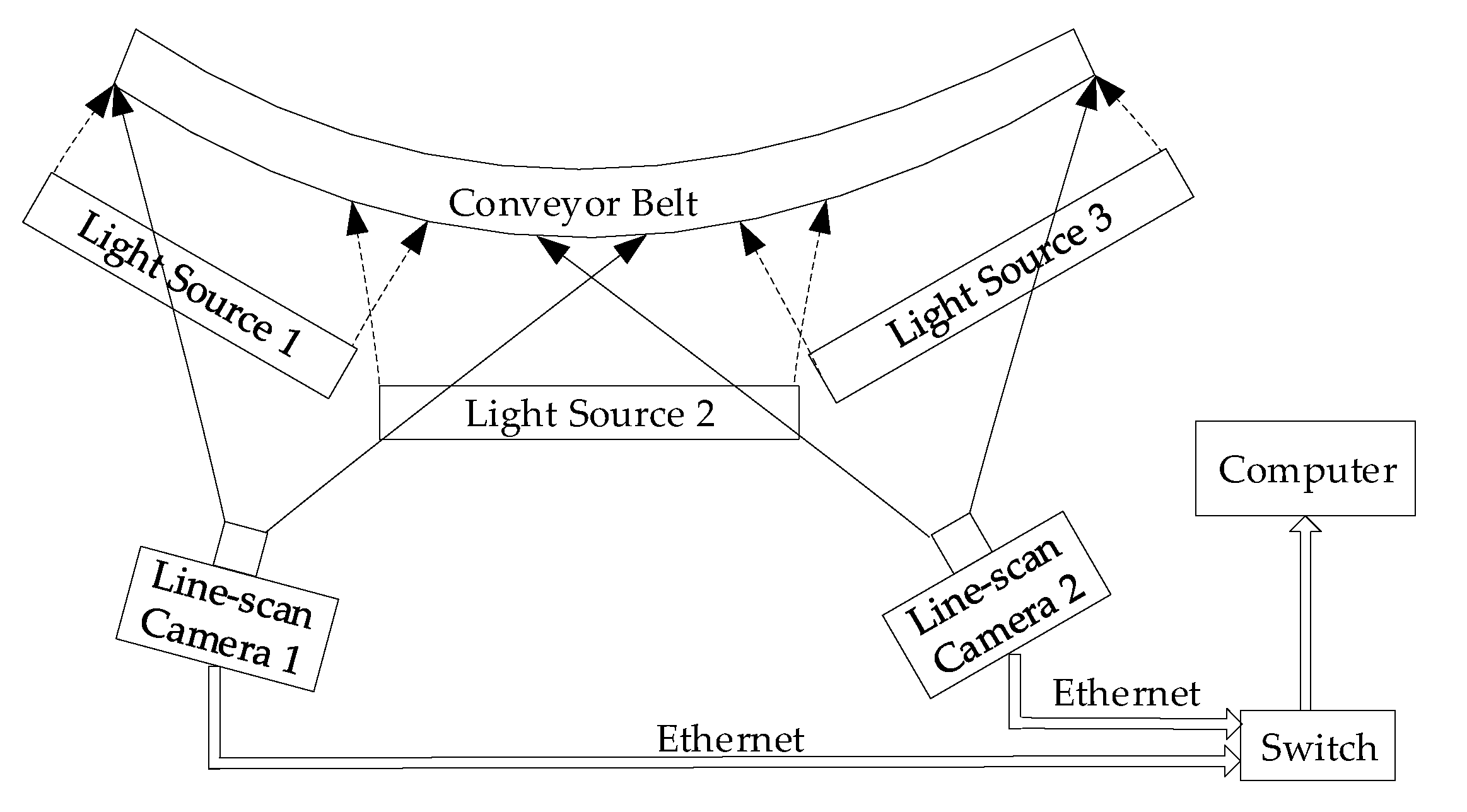
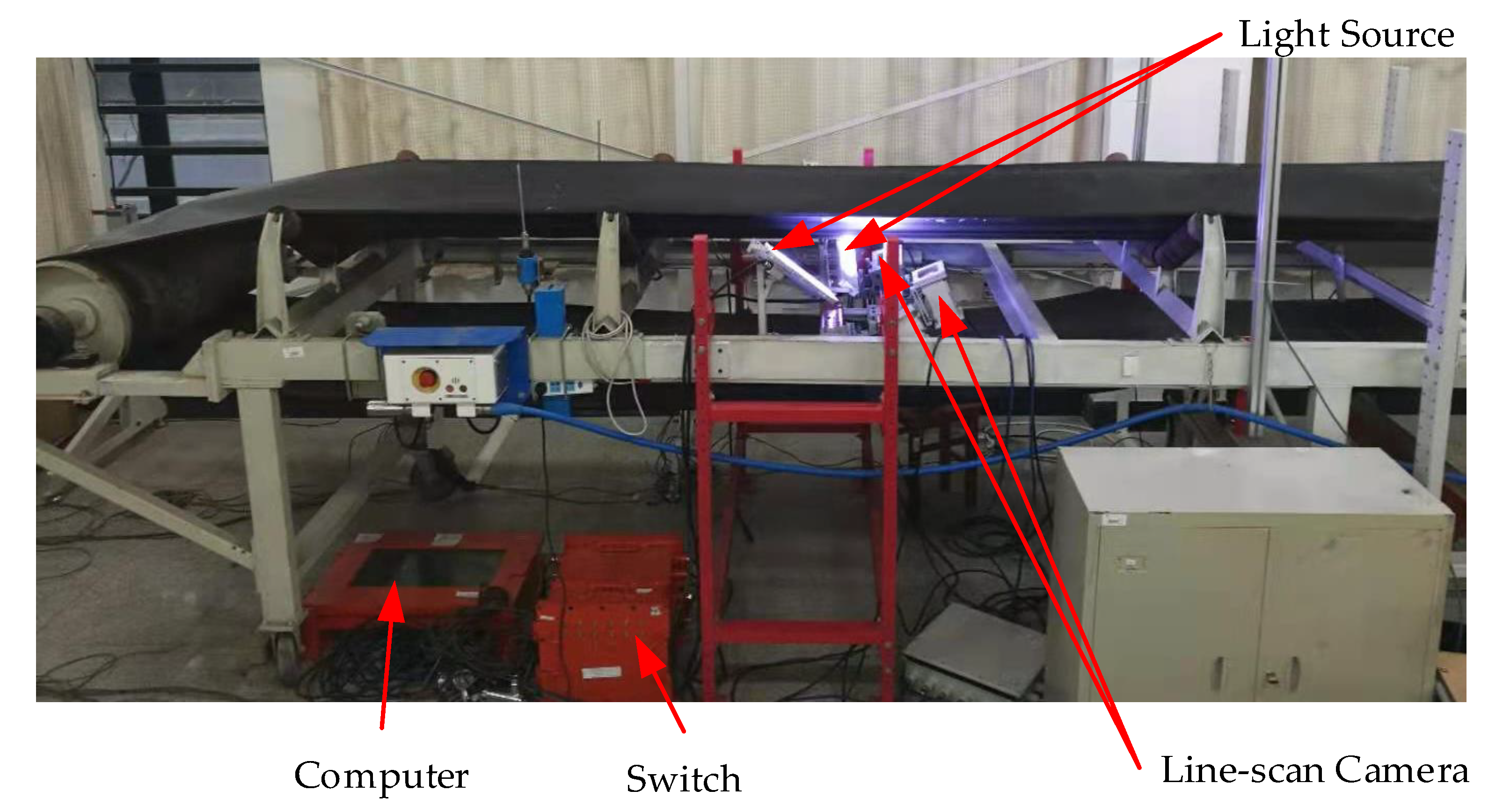
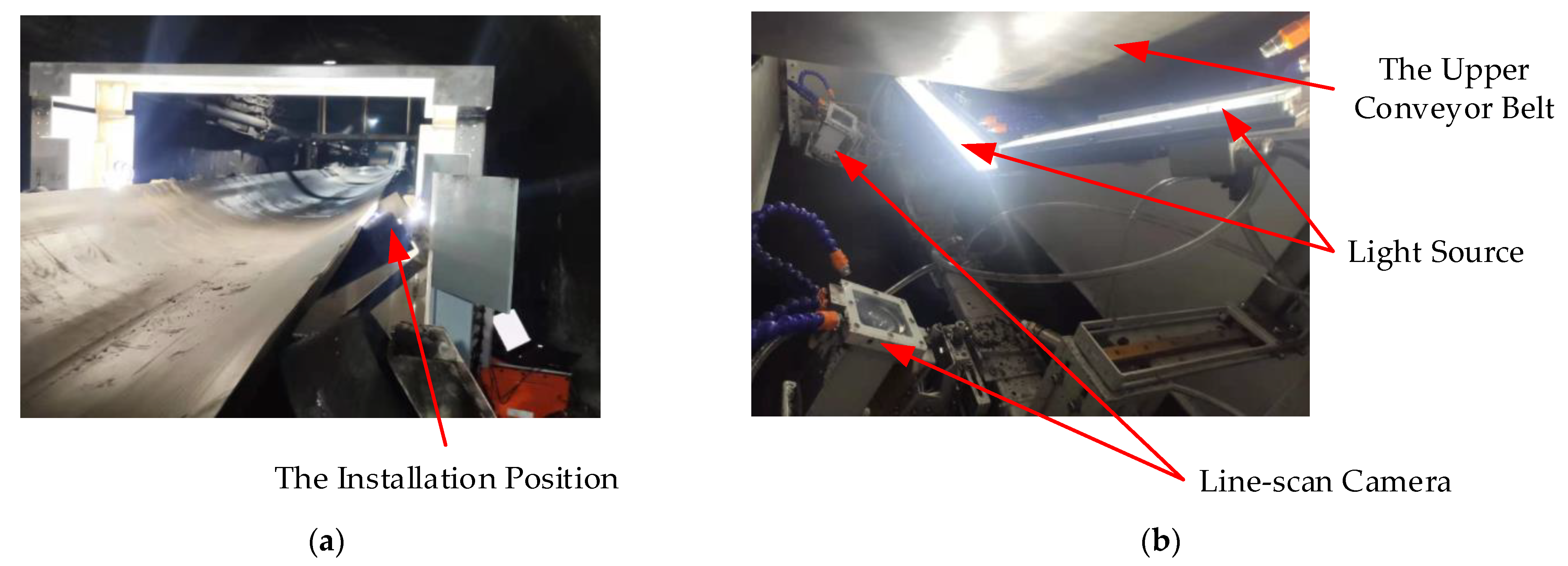
The multi-view conveyor belt surface fault online detection system based on machine vision comprises line-scan charge-coupled device (CCD) network cameras, linear light sources, Ethernet switch, and computer. The schematic diagram of the system components is shown in Figure 1.
The device produces diffuse reflection light when the light is emitted by a high brightness linear light source and irradiates on the surface of the conveyor belt. The light intensity of the diffuse reflection light is related to the surface characteristics of the conveyor belt [4,5,6]. The multi-view line-scan CCD camera senses the diffuse reflection light through line scanning. Each scan takes a line of images perpendicular to running direction of the conveyor belt and transmits it to the computer through Ethernet. The computer processes running image of the conveyor belt, analyzes and recognizes the conveyor belt fault, and gives a fault alarm or shutdown control signal when a fault is found.
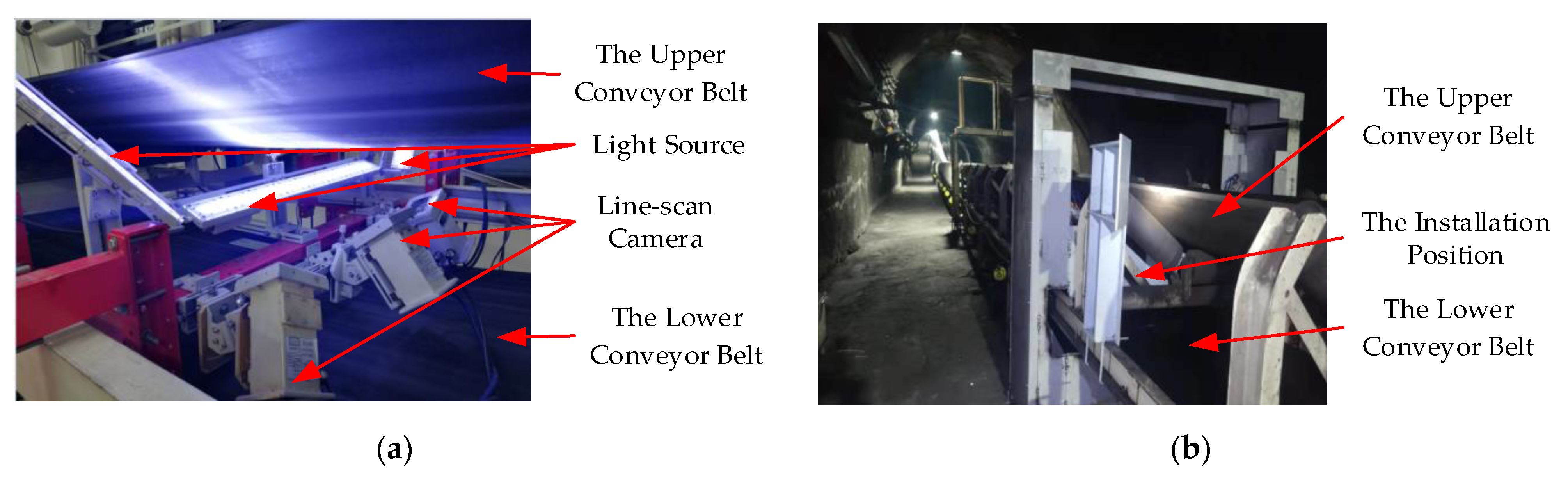
The structural characteristics of the conveyor limit the installation space of the camera. Generally, the camera can only be installed close to the conveyor belt. If the image of the lower surface of the conveyor belt is to be collected for fault detection, the camera can only be installed in the narrow space between the upper and lower belts, close to the lower surface of the conveyor belt. The distance is less than 40 cm, and the object distance is small, as shown in Figure 2. The width of the conveyor belt is generally 0.8–2.4 m. Because the cross-section is arc and the field of view is large, it is difficult to detect the width and accuracy of the conveyor belt with a single camera. It is necessary to use multiple cameras to acquire images in a multi-viewpoint manner by selecting appropriate installation position and installation postures to realize the conveyor belt without blind area coverage.
However, two adjacent images have overlapping regions that image the same conveyor belt content. Determining the two images’ overlapping regions can effectively reduce the processing range of image, reduce the amount of calculation, and improve the stitching speed. The geometric shape of the conveyor belt and the influence of factors such as the parameters, installation position, and posture of the multi-view camera make it difficult to determine the exact overlapping region.
3. Materials and Methods
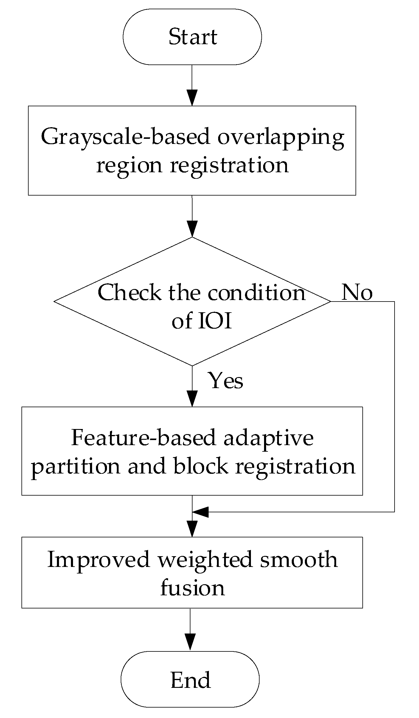
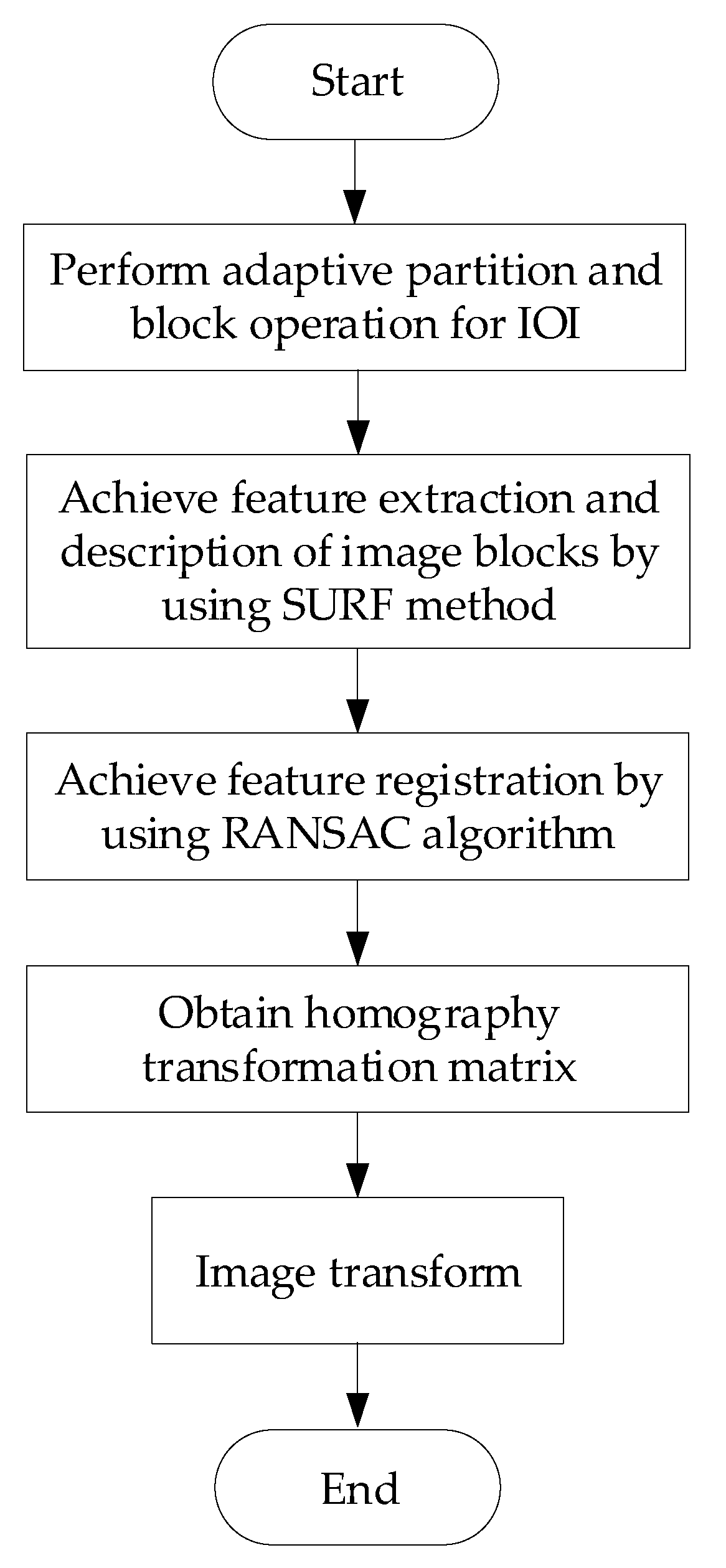
The adaptive multi-view image mosaic (AMIM) method proposed in this paper realizes multi-view conveyor belt surface fault online detection image stitching by the following sub-methods: grayscale-based overlapping region registration, the division of the IOI (image of interest), feature-based adaptive partition and block registration, improved weighted smooth fusion. The flow chart of the AMIM method is shown in Figure 3.
3.1. Grayscale-Based Overlapping Region Registration
3.1.1. Overlapping Region Estimation
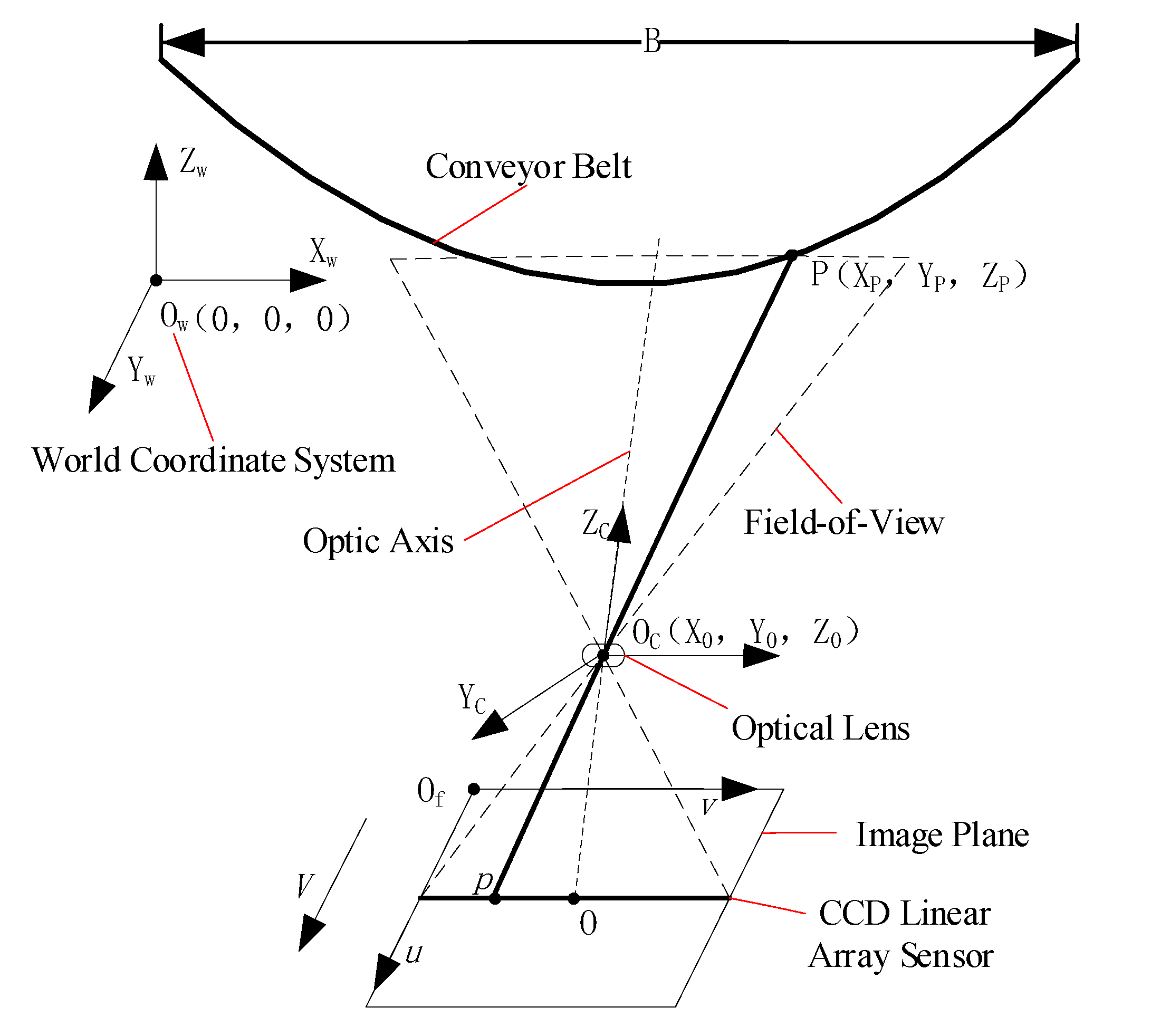
The overlapping region estimation model of 2 adjacent images is established according to the geometry of the conveyor belt and the parameters, installation position, and posture of multi-view cameras. For a conveyor belt, the horizontal distance between its two ends is set as B, the speed is V. Suppose it runs smoothly and at a uniform speed. The sensor pixel size of the line-scan camera is w, the number of pixels is n, the line sampling frequency is fh, and the lens focal length is f. For the conveyor belt, the world coordinate system Ow-XwYwZw is established. The Xw axis passes through the bottom end of the arc cross-section of the conveyor belt and is parallel to the ground, and the direction is from left to right. The Zw axis passes through the leftmost endpoint of the arc cross-section of the conveyor belt and is perpendicular to the ground, and the direction is from bottom to top. The intersection point Ow of the Xw axis and the Zw axis is the origin, and the origin coordinate is (0, 0, 0). The direction of V is the same as the Yw axis. Then, in the world coordinate system Ow-XwYwZw, the coordinate of the camera installation position Oc is (X0, Y0, Z0), the unit is millimeter; the camera installation posture is (α, β, γ), the unit is degrees (°). In the line-scan camera imaging process, the space points are projected onto the image sensing pixels to form an image, and the image pixel coordinate system is Of-uv. The imaging schematic diagram of the line-scan camera is shown in Figure 4.
The static imaging of a line-scan camera can only obtain the one-dimensional image of the conveyor belt. Because of the relative motion between the conveyor belt and line-scan camera, the line-scan camera can obtain a two-dimensional image of the conveyor belt by dynamic imaging. Suppose that the coordinate of any point P on the conveyor belt in the world coordinate system Ow-XwYwZw is (XP, YP, ZP), and the coordinate of the point P imaged in the image pixel coordinate system Of-uv is (u, v). According to the fundamental relationship of the perspective projection geometric imaging model of the imaging characteristics of the area-scan camera and the line-scan camera [23,24], one can obtain the dynamic imaging model of the line-scan camera, is seen in Equation (1):
where v0 is the pixel coordinate value of the main imaging point O of sensor pixel center of the line-scan camera, which can be generally set as v0 = n/2. f′ = f/w. V′ represents the relative motion between the conveyor belt and the line-scan camera in each image acquisition cycle, satisfying V′ = V/fh. Compared with V′, the relative motion of the conveyor belt caused by vibration and offset can be ignored. The results show that △v is the imaging distortion, and △v increases gradually from v0 to both sides. The Equation is as follows:
where k1, k2, and k3 are distortion parameters, which can be obtained by camera calibration.
In Equation (1), a1, a2, a3, b1, b2, b3, c1, c2, c3 are the elements of the rotation matrix of rigid body transformation between the world coordinate system Ow-XwYwZw and the line-scan camera coordinate system Oc-XcYcZc. The rotation matrix is an orthogonal matrix related to the camera installation posture (α, β, γ), as shown in Equation (3).
In Equation (1), the constraint condition ZP = g(XP) is the equation of conveyor belt arc cross-section in the world coordinate system by polynomial curve fitting.
Let the range of the conveyor belt content corresponding to the overlapping region of 2 adjacent images in the Xw axis direction of the world coordinate system be [XP1, XP2]. The overlapping region of 2 adjacent images only considers the v axis coordinates of image pixels. Let the pixel range of the overlapping region of the left image be [v1, n]. Let the pixel range of the overlapping region of the right image be [1, v2]. According to Equation (1), the overlapping region estimation model can be further established, which satisfies the relationship of Equation (4):
where, X01, Y01, Z01 and X02, Y02, Z02 are the installation position coordinates of the cameras corresponding to the 2 adjacent images, and a1, a3, c1, c3 and a1′, a3′, c1′, c3′ are the elements of the rotation matrix of the cameras corresponding to the 2 adjacent images. When v is v1, n, 1, and v2, the values of Δvv = v1, Δvv = n, Δvv = 1, and Δvv = v2 are the values of Δv, respectively. The overlapping region of 2 adjacent images can be estimated by solving the values of unknown variables v1, v2, Xw1, and Xw2.
3.1.2. Overlapping Region Registration
Because the range of overlapping region obtained by the overlapping region estimation model is a rough estimation, it is necessary to carry out overlapping region registration. We used the grayscale-based method with gray correlation analysis to measure the correlation between the reference pixel and the comparison pixel in the local area of the image. We can find the position with a higher gray correlation degree in the estimated overlapping region and realize the overlapping region registration.
There are 2 adjacent m × n size images—the gray value of the left image pixel is f1(u,v), and the gray value of the right image pixel is f2(u,v), where u is the row coordinate, u∈[1,m], v is the column coordinate, v∈[1,n]. The overlapping region range of the left and right images estimated is [v1,n] and [1,v2]. Registration of overlapping regions can be divided into the following steps:
Step 1: Select the region image whose column coordinates are v∈[v1−L,n] in the left image, and select the region image whose column coordinates are v∈[1,v2 + L] in the right image, where L is the deviation value.
Step 2: Calculate the mean of pixels of each column for the 2 regional images obtained. The Equation is as follows:
where img1(v) and img2(v) are the mean of pixels in column v.
Step 3: Affected by uneven illumination, weak imaging dark regions can appear at the edge of the image. To overcome its influence on stitching, for the left image, starting from v = n, one must look for the first one that satisfies img1(v) ≥ Td column by column in a descending manner and denote it as d1, d1 ≥ v1. For the right image, starting from v = 1, one must look for the first column that satisfies img2[v] ≥ Td column by column in an increasing manner and denote it d2, d2 ≤ v2; Td is the threshold. For the columns of the left image v∈[d1 + 1,n] and the right image v∈[1,d2−1], the gray correlation degree calculation is not performed, and the corresponding gray correlation degree εl or εr is assigned the value of zero.
Step 4: The reference sequence Xl0, Xr0 and comparison sequence Xl1, Xr1 were determined.
where k is an odd number.
For 2 images, take the current pixel img1(p) and img2(q) of the column mean as the center, and take k consecutive data to form a group of comparison sequences, where p∈[v1−L, v1 + L], q∈[v2−L, v2 + L]. The k consecutive data centered on img1(p) and img2(q) are divided into a group of comparison sequences as follows:
Step 5: The average processing is used to dimensionless each group of sequence data.
where “mean” means to get the average value of the sequence data.
Step 6: Calculate the difference sequence ∆l, ∆r, the maximum difference wl1, wr1, the minimum difference wl2, wr2.
where “max” and “min” represent the maximum and minimum values in the sequence data, respectively.
Step 7: Calculation of gray correlation coefficient and .
where i = 1, 2, …, k, ρ = 0.5.
Step 8: Calculation of gray correlation degree and .
Step 9:p = p + 1. If p satisfies the range of p∈[v1−L,v1 + L], continue to calculate the gray correlation degree εl with img1(p) as the current pixel according to step (4). q = q + 1. If q satisfies the range of q∈[v2−L,v2 + L], continue to calculate the gray correlation degree εr with img2(q) as the current pixel according to step (4).
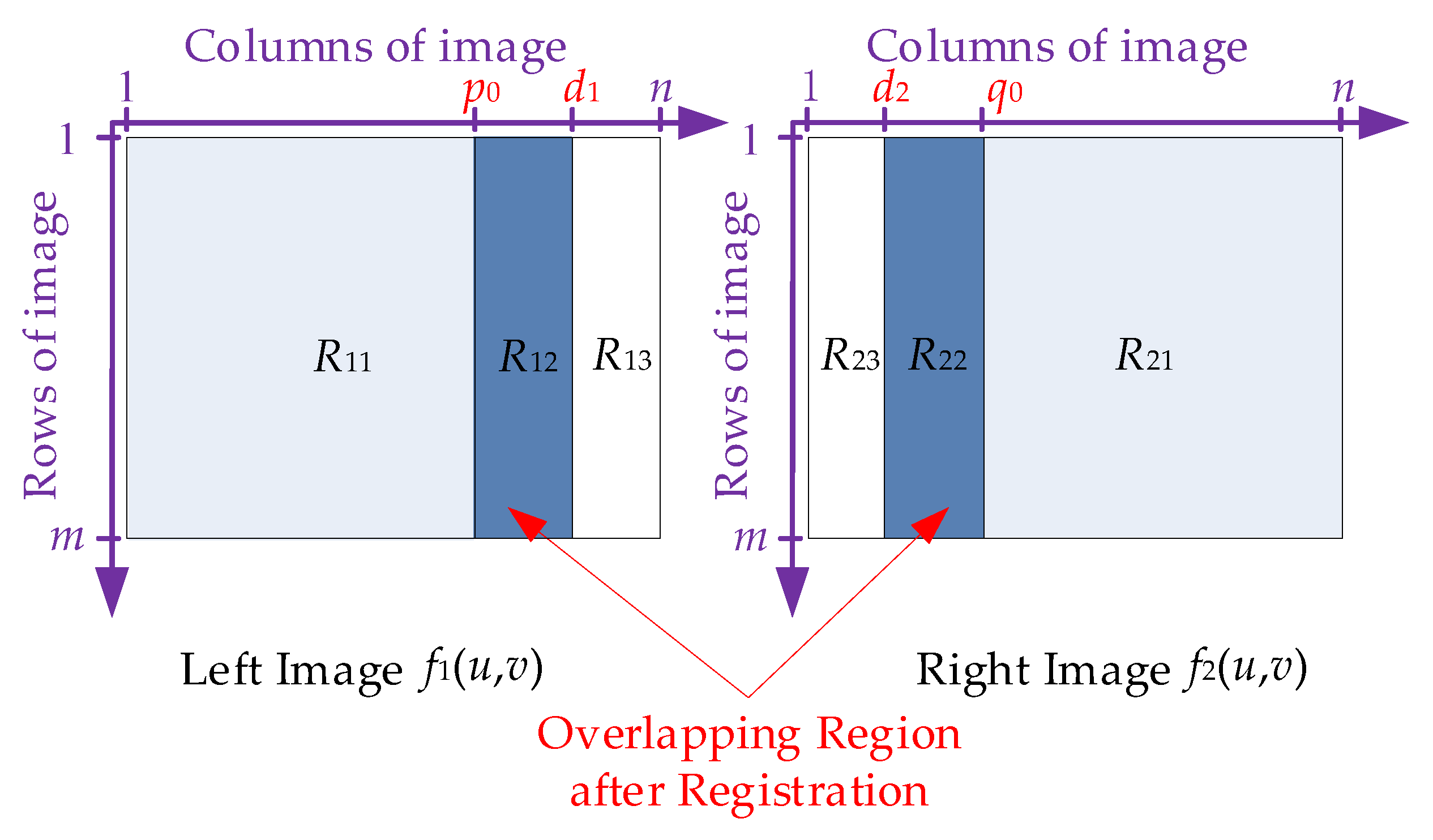
Step 10: Calculate the p value corresponding to the maximum value of εl and record it as p0. Calculate the q value corresponding to the maximum value of εr and record it as q0. Then, the range of overlapping region of the left image is determined as u∈[1,m], v∈[p0,d1], and the range of overlapping region of the right image is determined as u∈[1,m], v∈[d2,q0], and the overlapping region registration is completed.
As shown in Figure 5, regions R12 and R22 are the overlapping regions after registration, regions R11 and R21 are the non-overlapping regions, and regions R13 and R23 are the dark regions.
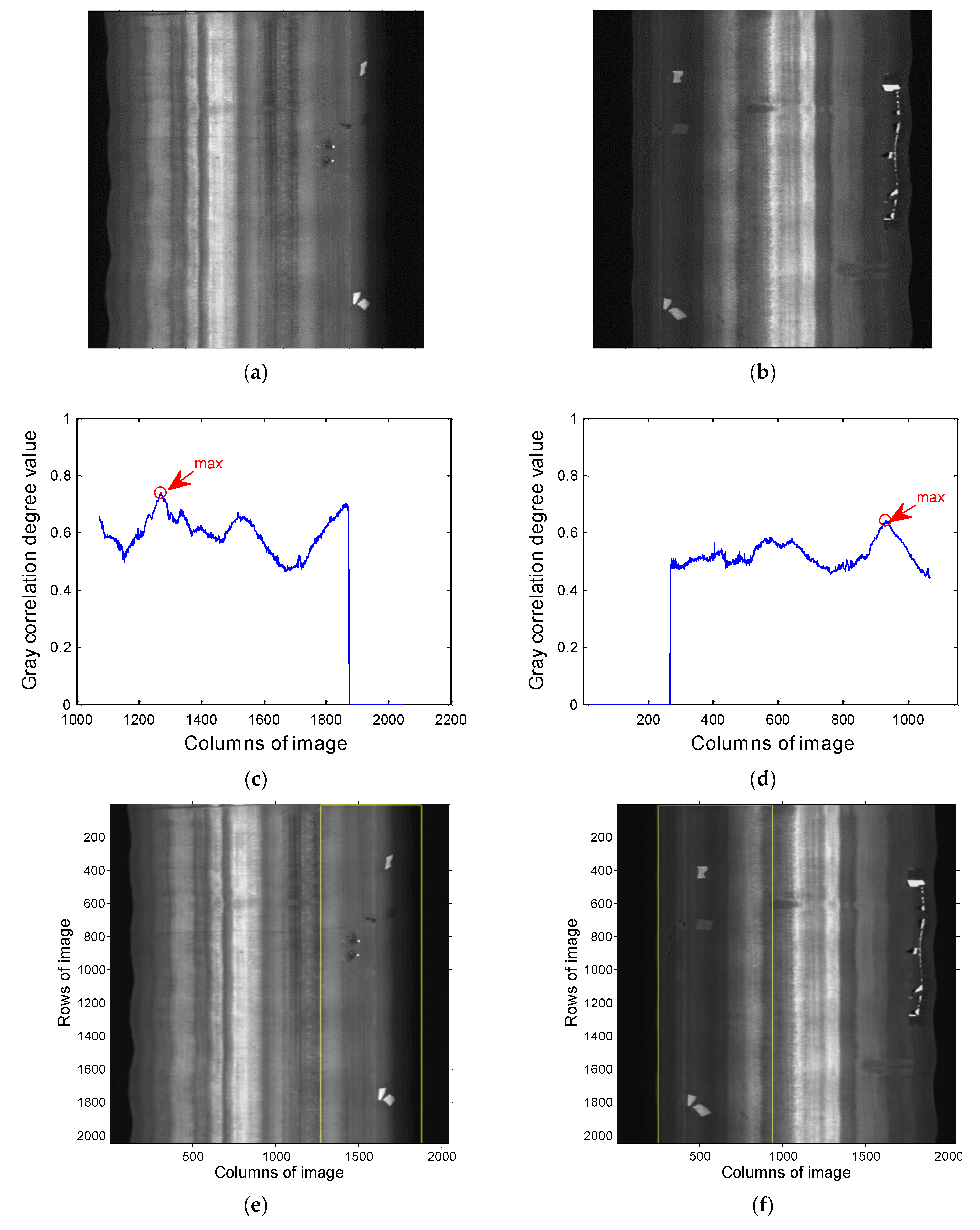
Select 2 adjacent images in the multi-view conveyor belt images. The image size is 2048 × 2048, as shown in Figure 6a,b. When L = 800, k = 353, Td = 44 (Td as half of the mean of image pixels), carry out the method in this paper, and obtain the curves of gray correlation degree εl and εr, as shown in Figure 6c,d. It can be seen that the value range of the correlation degree is [0,1]; the maximum value of the correlation value is used to register the overlapping region. The left and right image registration overlapping regions are [1269,1886] and [245,932], respectively. The registration of overlapping region is shown in Figure 6e,f.
3.2. The Division of The IOI
It is difficult to detect, select, and match feature points in image mosaic of multi-view conveyor belt surface fault online detection, which makes it impossible to use the feature-based method for more accurate image registration. Generally, the useful feature points of the conveyor belt are mainly distributed in the regions such as stripes caused by moving friction, conveyor belt joints, defects, etc. This paper uses an IOI detection algorithm to divide the IOI and the non-IOI image to improve feature-based registration effectiveness.
For the i-th image of m × n size images collected from N viewpoint, let the gray value of image pixel be fi(u,v), and the overlapping region range be u∈[1, m], v∈[va, vb]. The detection algorithm of the IOI is as follows: if the value of any i∈[1, N] satisfies Ei ≥ TE, where TE is the threshold, then the N images to be stitched are considered to be the IOIs with apparent features; otherwise, they are the images with no apparent features. The image evaluation parameter Ei is calculated as follows:
where k1 and k2 are proportional coefficients, which represent the contribution degree of factors and satisfy k1 + k2 = 1. Generally, k1 and k2 can be set to 0.5. HMi(u) is the mean vector of row pixels, and Fi is the mean of image pixels, calculated as follows:
VDi(v) is calculated as follows:
where VMi (v) is the mean vector of column pixels, which is calculated as follows:
3.3. Feature-Based Adaptive Partition and Block Registration
For the IOI, the feature-based adaptive partition and block registration method is further used to improve stitching accuracy. The IOI is segmented adaptively to improve and enhance the efficiency and real-time stitching. The specific operation steps are as follows:
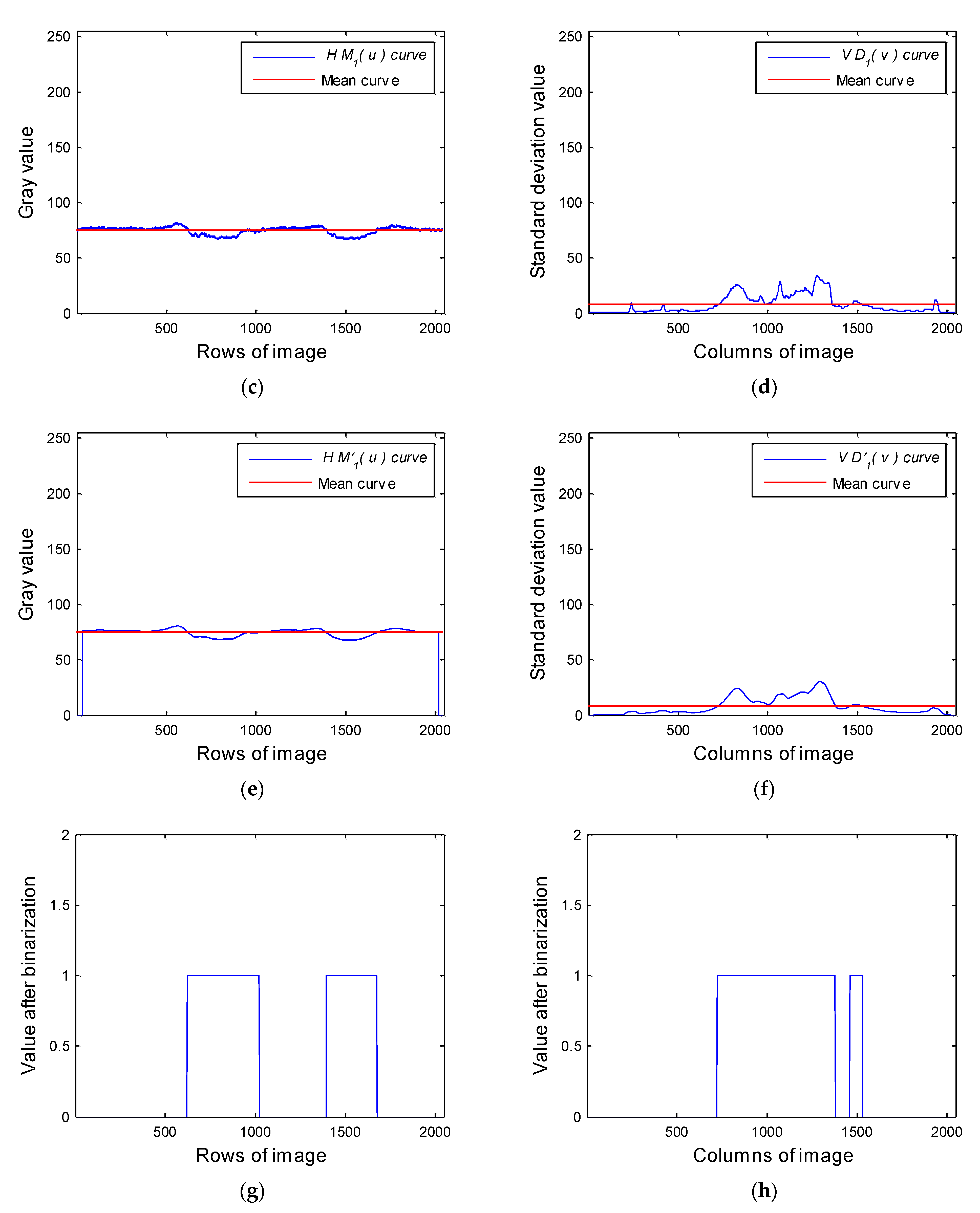
Step 1: A binarization curve is generated for the image partition of interest.
Select the HMi(u) curve and the VDi(v) curve described in Equation (15) and Equation (17). Construct a one-dimensional filter window with the size of Lf, and Lf is an odd number. Slide the filter window on the HMi(u) curve and VDi (v) curve, respectively. The mean of Lf pixels is taken as the value of the center pixel of the window. The HM′i(u) curve and VD′i(v) curve are obtained after the mean filtering. Then, perform binarization processing according to the following Equation to generate a binarization curve.
where Fi is the mean of HMi(u), as shown in Equation (16), and Vi is the mean of VDi(v), which satisfies:
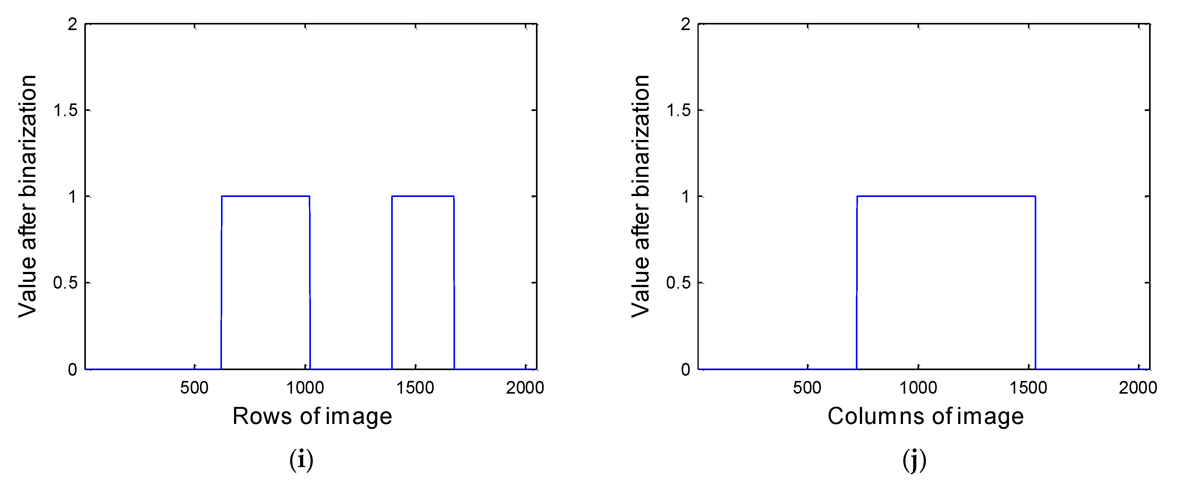
Step 2: Deal with the region of interest (ROI) of the binarization curve.
For BVDi(v) and BHMi(u) binarization curves, the region with a continuous value of “1” is found as the ROI of the curve, and the start position, end position, and length of the region are marked. The merging threshold TC of adjacent ROIs and the removal threshold TB of isolated small ROIs are set in order to solve the influence of scattered and small regions with continuous “1” on the partition effect of ROIs. Suppose the interval between 2 adjacent ROIs of BVDi(v) and BHMi(u) binarization curve satisfies the condition of less than TC. In that case, the 2 ROIs are merged and connected. If the length of the region is less than TB, the ROI is removed. After the processing, the binarization curves are BVDi′(v) and BHMi′(u).
Step 3: The ROI of IOI is generated and selected.
A template image with the same size as the overlapping region of the IOI is constructed, and its pixel value is gi (u,v).
where u∈[1,m], v∈[va, vb]; through Equation (23), the overlapping region of the IOI to be stitched is divided into 1 background region and Ki rectangular ROIs with effective feature points distribution.
If Ki ≥ 3, 2 ROIs with larger size are selected; otherwise, all ROIs are selected.
Step 4: The image block is generated and selected.
The ROI of the image is divided into Ni × Ni blocks, and the number of blocks is Bi. If Bi ≥ 3, 2 image blocks with larger standard deviation are selected; otherwise, all image blocks are selected.
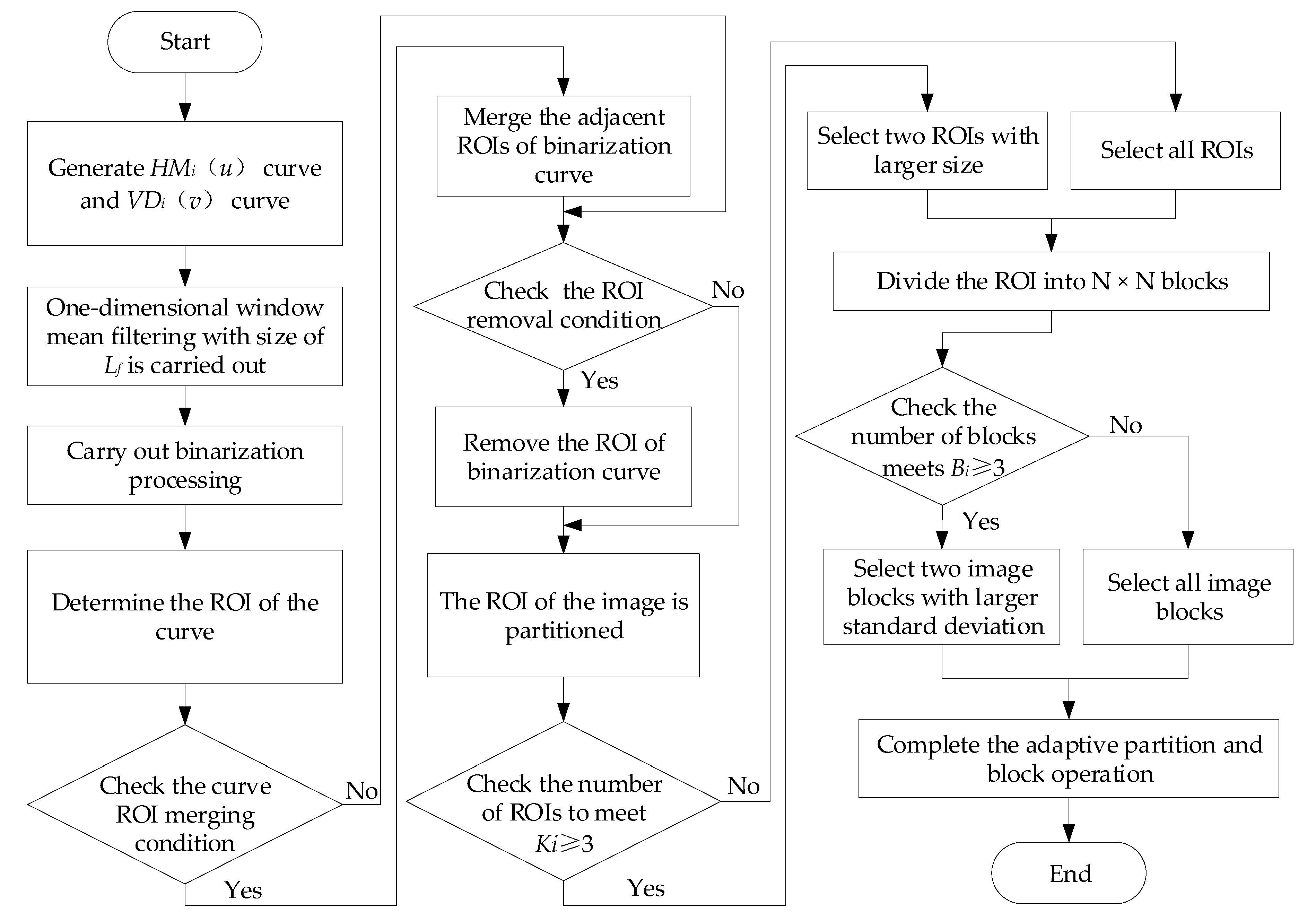
The flow chart of adaptive partition and block operation for the IOI is shown in Figure 7.
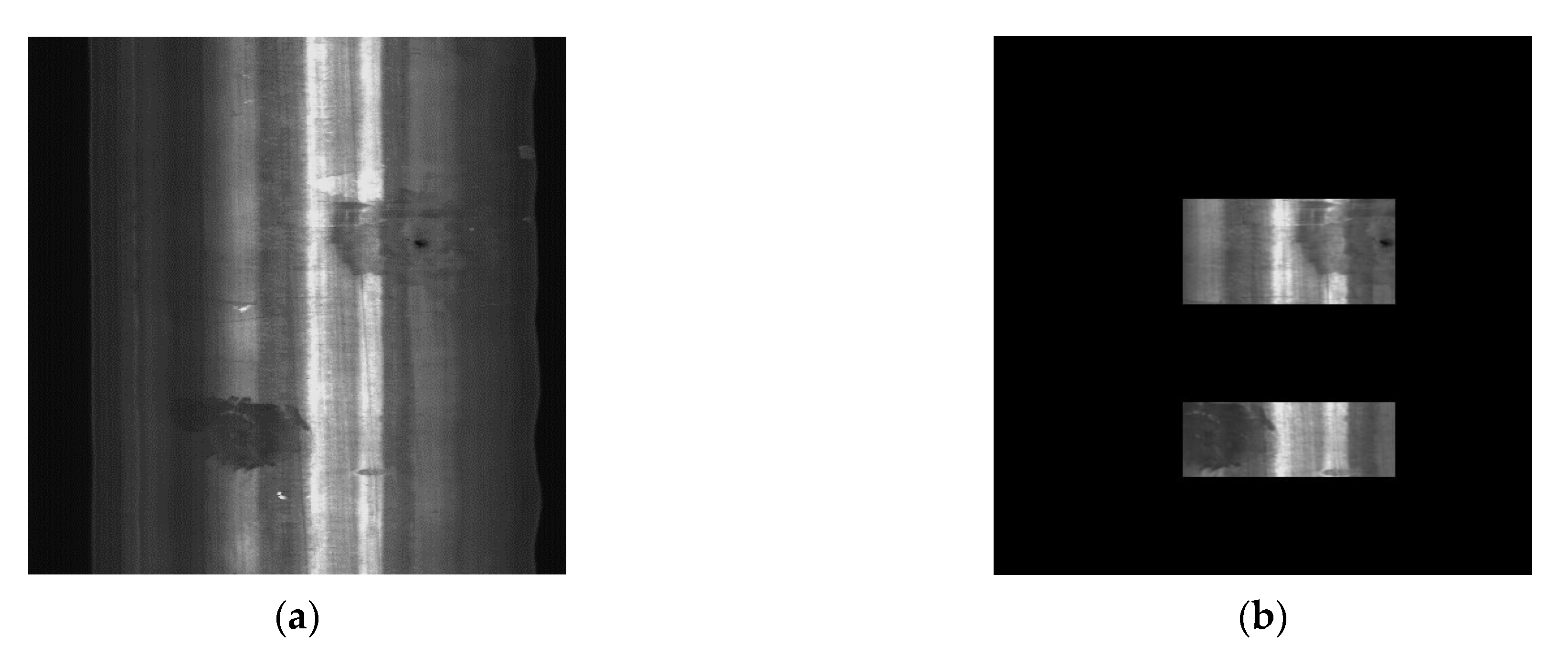
We verify the effect of partition operation for the IOI. An IOI with a size of 2048 × 2048 (assuming that the whole image is an overlapping region), as shown in Figure 8a, is partitioned. The curves of HM1(u) and its mean, VD1(v) and its mean are shown in Figure 8c,d. Construct a one-dimensional window template of size 61 (Lf = 61) for mean filtering. The curves of HM′1(u) and its mean are shown in Figure 8e. The curves of VD′1(v) and its mean are shown in Figure 8f.The binarization curves BHM1(u) and BVD1(v) are obtained as shown in Figure 8g,h, respectively. Suppose TC = 128 and TB = 128, the binarization curves BHM1′(u) and BVD1′(v) obtained after merging and removing operations are shown in Figure 8i,j, respectively. Finally, the ROI is partitioned, and the result is shown in Figure 8b. It can be seen from 8b that most of the defect information of the conveyor belt is contained in the ROI, which reduces the scope of image registration.
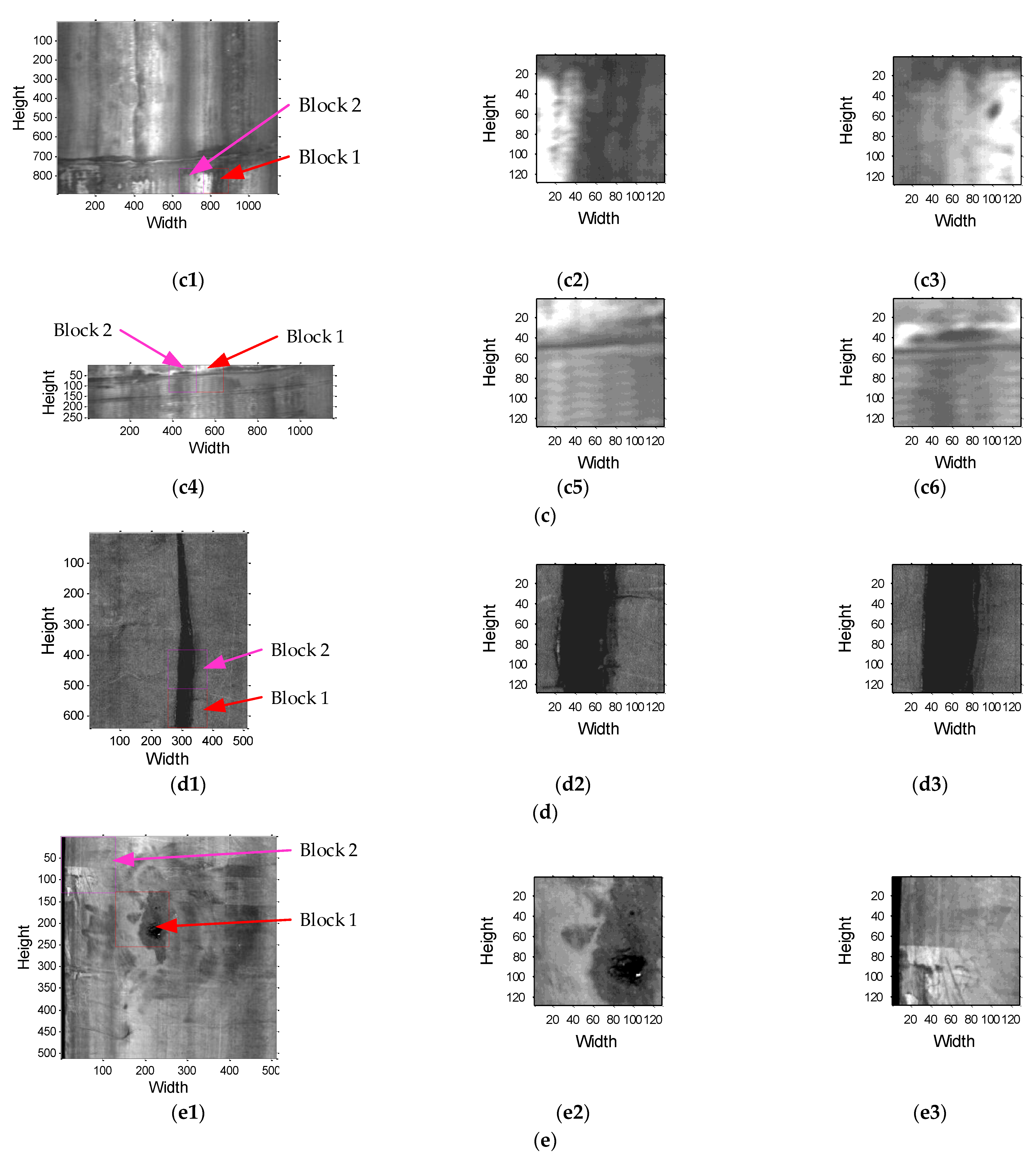
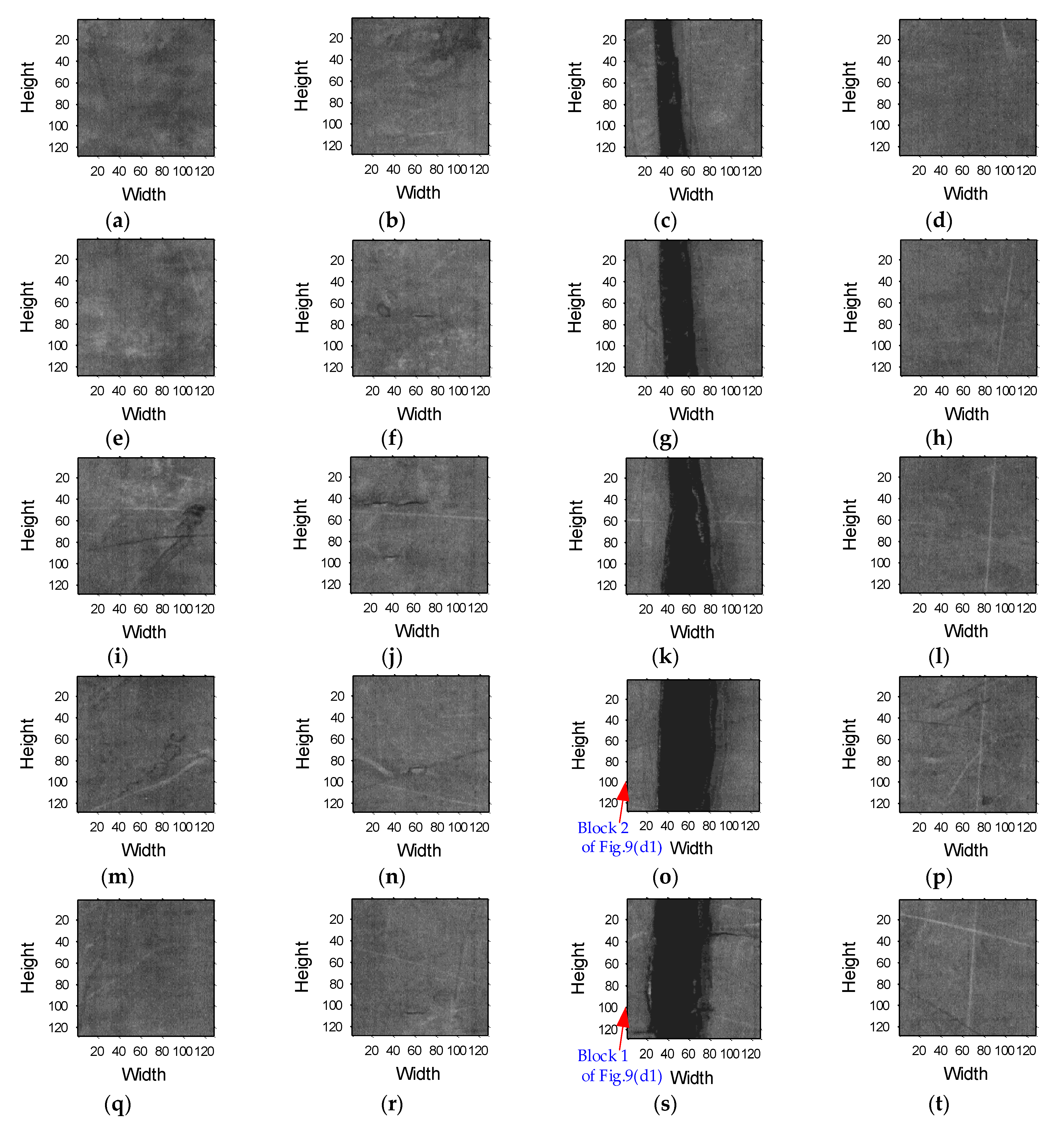
We further verify the effect of adaptive partition and block operation for the IOI. The original images are shown in Figure 9a. Lf = 61, TC = 128, TB = 128 are used to process the original image and extract the ROI, as shown in Figure 9b. The ROI image is selected and divided into 128 × 128 blocks. The selected ROI images are shown in Figure 9(c1,c4,d1,e1). The result of 128 × 128 blocks for Figure 9(d1) is shown in Figure 10. The position of the image block is represented by (ri, ci); ri and ci are the numbers of rows and columns of the image block arranged according to the matrix, respectively, satisfying ri ≤ Ri, ci ≤ Ci, Bi = Ri × Ci. The number of blocks shown in Figure 10 is 5 × 4. Then, select the image block with a larger standard deviation, as shown in Figure 9c–e, where Figure 9(d2,d3) are the image blocks with the largest standard deviation (Block 1) and the second-largest standard deviation (Block 2), and the positions in Figure 10 are (5,3) and (4,3), respectively. It can be seen that the separated image block contains a high amount of feature information, such as conveyor belt joint or surface fault, which is conducive to the extraction of useful features. The results of the ROI adaptive partition and block method are shown in Table 1.
To speed up the calculation, we use the SURF algorithm for feature extraction and description of the selected image block. The SURF algorithm includes the following operations: building the Hessian matrix for feature point extraction, building scale space, feature point location, feature point main direction assignment, feature point descriptor generation, and feature point matching. The random sample consensus (RANSAC) algorithm is used to eliminate the outer points and retain the inner points for image registration. The transformation matrix of the image is constructed through the matching point pairs. According to the transformation matrix obtained by feature registration, the corresponding image is transformed. Feature point matching uses the distance function (Euclidean distance) to retrieve the similarity between high-dimensional vectors. In this paper, the K-D tree algorithm is used. Firstly, the K-D tree is established for each image with the feature descriptor as the tree node information. Then, the K data closest to the corresponding feature points in the other image is searched using the feature points of 1 of the 2 images to be stitched to complete the initial matching of feature points. The flow chart of the feature-based adaptive partition block registration method is shown in Figure 11.
3.4. Improved Weighted Smooth Fusion
The improved weighted smoothing algorithm is used for image fusion to get the stitched image. The expression of the improved weighted smoothing algorithm is as follows:
where R11 and R22 are the non-overlapping regions of 2 adjacent images; R12 is the overlapping region; and ω1 and ω2 are the weights of corresponding pixels in the overlapping region, respectively, satisfying 0 < ω1, ω2 < 1 and ω1 + ω2 = 1. To ensure the continuity of overlapping region transition and effectively remove stitching marks, one calculates the weight according to the following equation:
4. Experiments and Results
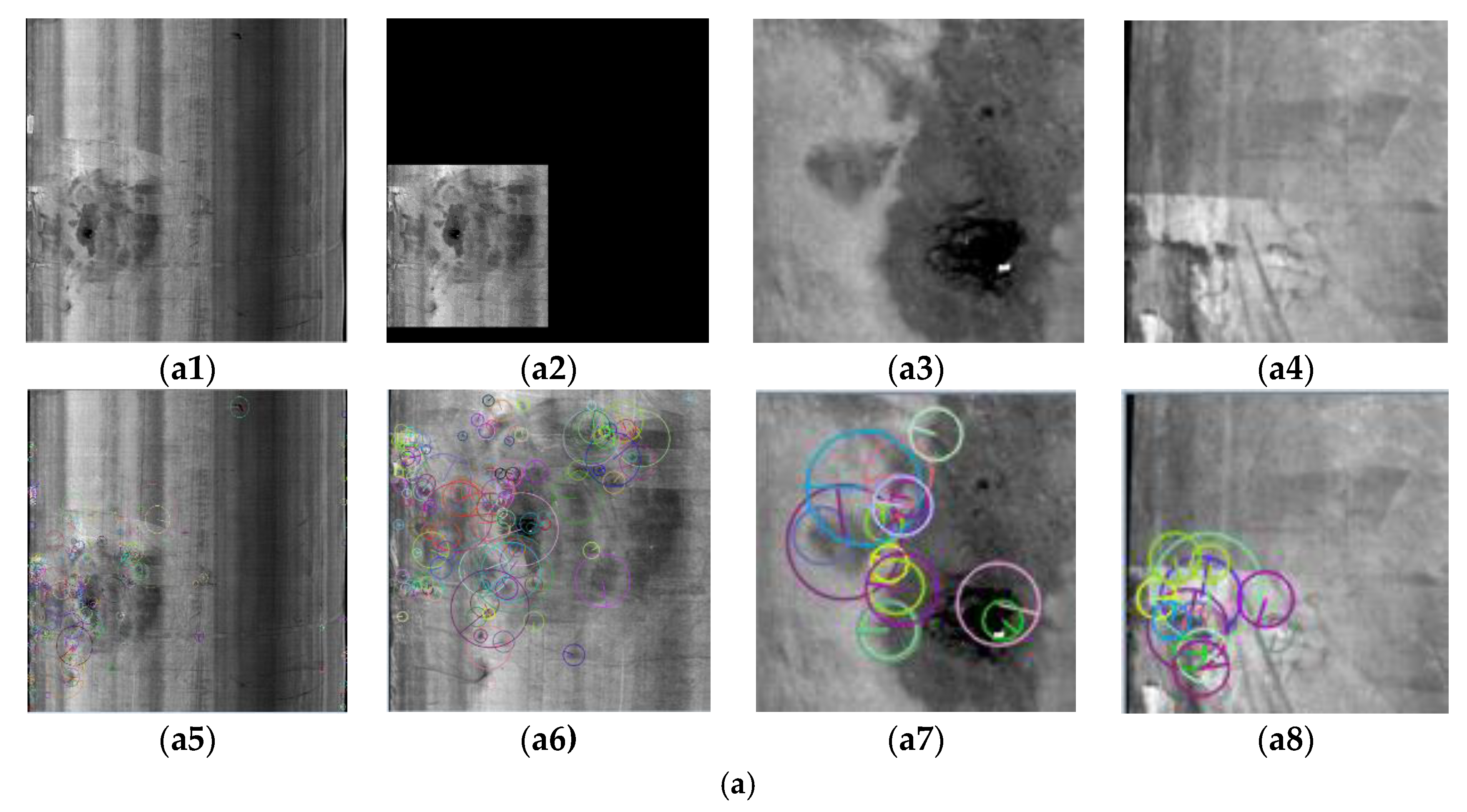
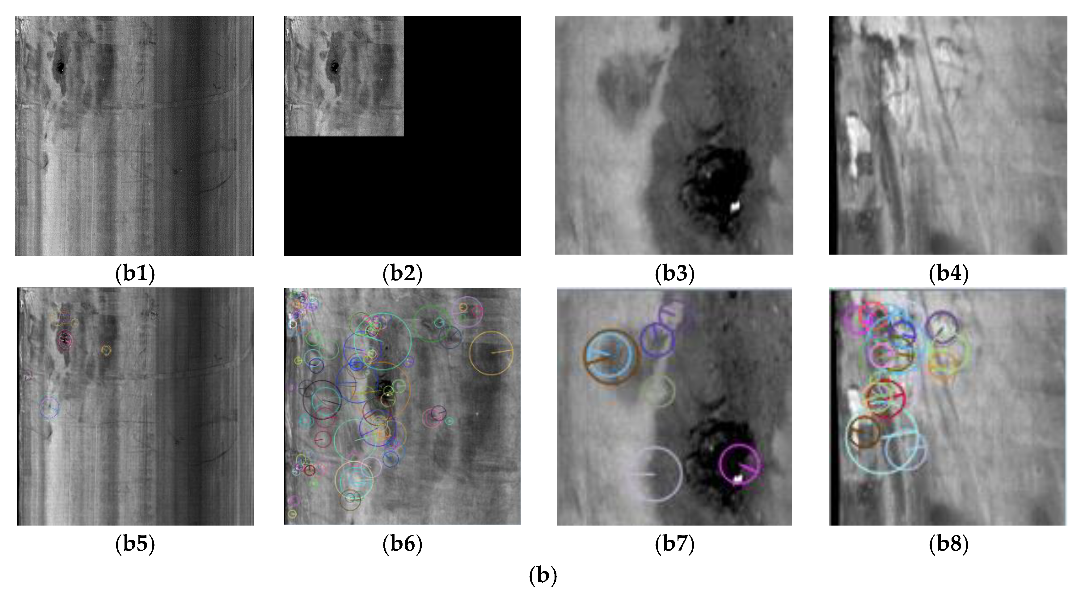
The experiment is carried out on the platform, as shown in Figure 12, in order to verify the effectiveness of the method proposed in this paper. Two 2048 × 2048 IOIs with the same surface damage content were selected, as shown in Figure 13(a1,b1). Simulation by using MATLAB software programming in Intel i5 CPU computer showed that the method was effective. The ROI images are shown in Figure 13(a2,b2). The block images are shown in Figure 13(a3,a4,b3,b4). For the original image, the ROI image, and the block image, the SURF algorithm with the Hessian matrix determinant response value of 1000 was used for feature extraction and description. Draw the circle on the image with the feature point as the center. The radius of the circle indicates the size of the feature point, and the straight line indicates the direction of the feature point. The feature points are described as shown in Figure 13(a5–a8,b5–b8).
The comparison of image feature extraction is shown in Table 2. It can be seen that the number of feature points extracted in the ROI of Figure 13(a1,b1) were 65.52% and 69.71% of the whole image, respectively. The number of feature points extracted from the ROI accounts for a high proportion of the number of feature points in the whole image, reflecting that the ROI is the feature point concentration region of the whole image. However, it took 40.48% and 37.18% of the total image time, respectively, which was less time-consuming. Although the number of feature points extracted from two image blocks was less than the ROI, the feature points extracted had larger feature values and significant features, which met easy registration requirements. Moreover, the two image blocks took less time. The total time was only 16 ms, which was 2.77% and 2.93% of the whole image time, respectively. It is thus suitable for fast registration.
For the two images of Figure 13(a1,b1), the different threshold values of Hessian matrix determinant response value, such as 500, 1000, 1500, and 2000, were used to extract the feature points of each image. The comparison in Table 3 shows that with the increase of the threshold value, the number of feature points extracted and the time consumed was reduced. However, the threshold value is important for the block image, because of the small image size. If the threshold value is too large, too few feature points are extracted in the block, which is not conducive to feature point registration. For example, when the threshold value was 2000, the number of feature points shown in Figure 13(b7) was only one. The threshold value of the Hessian matrix determinant response value can be selected as 1000 by comparison.
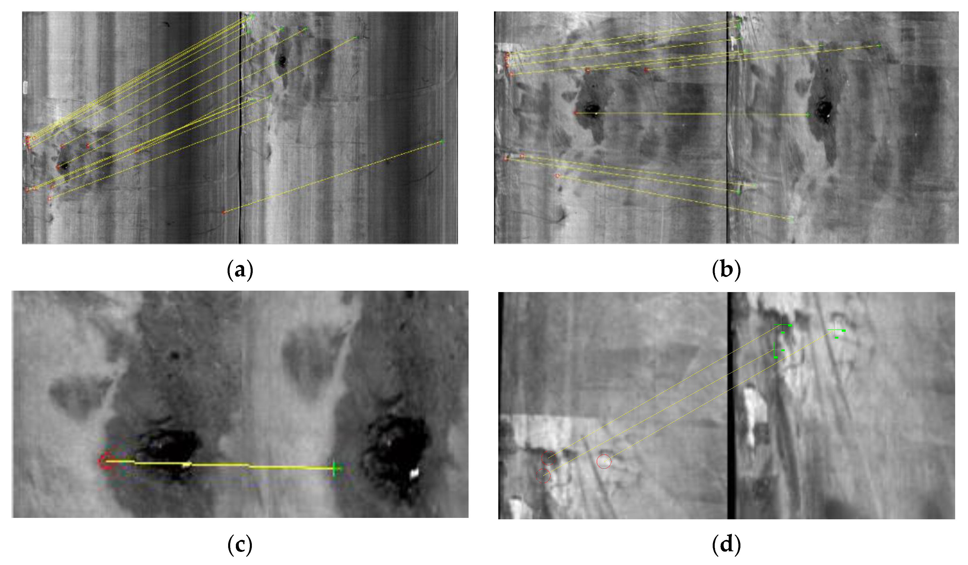
For the feature points extracted from the original image, ROI image, and block image, we used the RANSAC algorithm to complete the matching of feature points. The matching results are shown in Figure 14. The comparison of registration is shown in Table 4. It can be seen that a sufficient number of registration feature point pairs can be obtained from block images. The time of registration processing on an Intel i5 CPU computer was 5 ms, which was 41.67% of the total image time.
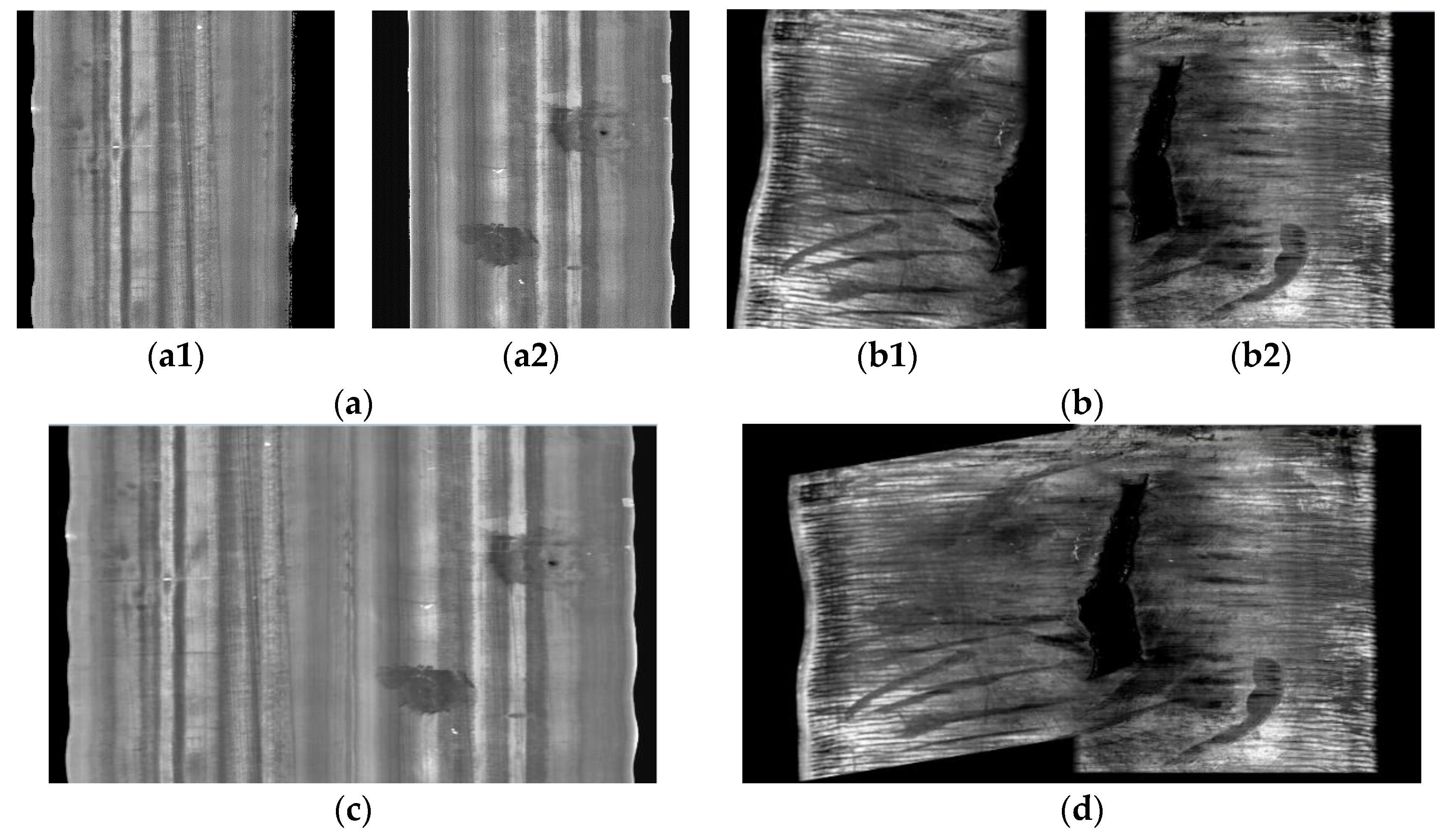
The proposed method was applied in the mine for conveyor belt surface fault online detection, as shown in Figure 15. To further verify the effectiveness of the AMIM method, we selected two groups of images collected by two line-scan cameras with different viewpoints. The image size was 2048 × 2048, as shown in Figure 16a,b. When L = 800, k = 353, Td = 44 (Td as half of the mean of image pixels), the overlapping regions of left and right images in Figure 16a were [1519,1788], [236,397], and the overlapping regions of left and right images in Figure 16(b) were [1526,1784], [257,546]. The parameters were set as TE= 20, Lf = 61, TC = 128, TB = 128. The evaluation parameters E of the IOI calculated from the image registration overlapping region in Figure 16a were 11.22 and 8.14, respectively. The evaluation parameters E were calculated by Equation (14). According to the detection algorithm of the IOI, the images in Figure 16a were identified as the non-IOI. For the overlapping region estimated from the image in Figure 16b, the evaluation parameters E of the IOI calculated were 29.06 and 36.97, respectively. The images in Figure 16b were identified as the IOI. Only for the Figure 16b, using 128 × 128 block size, was the feature-based adaptive partition block registration method carried out. Finally, the improved weighted smoothing algorithm was used for image fusion, and the stitched image was obtained, as shown in Figure 16c,d. The subjective evaluation of the stitched image shows that the stitching effect of the AMIM method is good.
The AMIM method is evaluated from the registration rate and running time to verify the effectiveness of our method more objectively.
The registration rate measures the accuracy of the matched feature points.
where Z is the registration rate, c1 is the number of mismatched feature pairs, and c2 is the number of feature pairs in the RANSAC algorithm.
The comparison between the AMIM method and other methods is shown in Table 5. For the images in Figure 16a, SIFT and SURF method cannot get the correct registration feature points and cannot realize the accurate image stitching operation on the basis of features. However, the AMIM method does not use the feature-based registration method after identifying the image as the non-IOI. It uses the overlapping region of registration to stitch the image directly. For the image in Figure 16b, although the number of feature points extracted by our method was small, the registration rate was high, reaching 97.67%. The average time of stitching two adjacent images was less than 500 ms. Thus, our method ensures image stitching accuracy, reduces the registration time, and improves image stitching efficiency. Therefore, our method has advantages in the process of multi-view conveyor belt image stitching.
5. Conclusions
Correct operation of the conveyor belt is very important for production and staff safety. The multi-view conveyor belt surface fault online detection system based on machine vision can provide a sufficient guarantee. This paper proposed an adaptive multi-view image mosaic method based on the combination of grayscale and feature to improve the accuracy and real-time of image mosaic and realize the multi-view conveyor belt surface fault online detection. Compared with the traditional mosaic methods, the proposed method has the following improvements and advantages:
The overlapping region of two adjacent images is preliminarily estimated by establishing the overlapping region estimation model, and then the grayscale-based method is used to register the overlapping region.
For the collected image, the IOI detection algorithm is used to divide it into the IOI and the non-IOI, and different registration methods are used.
For the IOI, its overlapping region may contain the fault information of the conveyor belt. The feature-based partition and block registration method is used to register the images more accurately, the overlapping region is adaptively segmented, the SURF algorithm is used to extract the feature points, and the random sample consensus RANSAC algorithm is used to achieve accurate registration. It is easy to realize the accurate measurement of the geometric shape of the fault, and it is conducive to the accurate and reliable detection and evaluation of the health status of the conveyor belt.
For the non-IOI, its overlapping region almost does not contain the fault information of the conveyor belt, and the features are not obvious. It is easy to have the wrong registration by using the SIFT algorithm, SURF algorithm, and other feature-based registration methods, and the registration rate is even 0%. Thus, they cannot obtain the right result, and the process is time-consuming, which is not conducive to real-time online detection. Accurate registration is not performed on the adjacent non-IOIs, which improves the accuracy and real-time of stitching.
The improved weighted smooth fusion algorithm is used to fuse the images to realize image stitching.
The experimental results show that when the SURF algorithm is used to extract and describe the block image features, the threshold value of the Hessian matrix determinant response value is 1000, which is better compared with 500, 1500, and 2000. It has the advantage of extracting enough feature points and consuming less time. Enough feature points can be extracted from the block image, and the features are significant, which is easy to register accurately. Compared with the whole image registration, it takes less time. The results of the experimental analysis showed the usefulness of the proposed method. The stitching effect is better compared with the SIFT and SURF algorithms. Simultaneously, it can reduce the amount of stitching calculation and the time of the stitching process, and the registration rate is high. The registration rate can reach 97.67%, and the average time of stitching two adjacent images is less than 500 ms. It is suitable for conveyor belt surface fault online detection. In addition, this method can also provide a reference for other application types of image mosaic.
The proposed method was applied in the mine for conveyor belt surface fault online detection and can be extended to port, electric power, metallurgy, chemical industry, and other fields for conveyor belt surface fault online detection. In the future, we will study the methods of accurate and reliable detection and evaluation of conveyor belt health. In order to improve the detection performance, we can further use the hybrid imaging method combining thermal imaging [25] and visible light imaging to explore ways to realize the fusion of heterogeneous images and multi-view image mosaic at the same time. It is also valuable to explore the application of deep learning in conveyor belt fault detection [26].
Multi-view is widely used in machine vision-based detection and has played an important role. The proposed method in this paper can be used in industry, agriculture, medical, and other fields of fault detection using the multi-view method [27,28,29,30]. Compared with other improved image mosaic methods, the proposed method is more suitable for solving the problem of conveyor belt surface fault online detection. For example, the IOI detection algorithm is proposed on the basis of the characteristics of the conveyor belt image, and it may not be adaptable to other detection object images for different applications. However, for other applications, the proposed method in this paper has a reference value for image mosaic problems that need to take into account both accuracy and real-time.
Author Contributions
Conceptualization, R.G.; methodology, R.G.; validation, R.G. and X.L.; formal analysis, R.G.; resources, C.M.; data curation, X.L.; writing—original draft preparation, R.G.; writing—review and editing, X.L.; supervision, C.M.; project administration, R.G.; All authors have read and agreed to the published version of the manuscript.
Funding
This research was funded by the National Natural Science Foundation of China (grant no. 51504164), Key Scientific and Technological Support Projects of Tianjin Key R&D Program (grant no. 18YFZCGX00930), the Tianjin Natural Science Foundation (grant no. 17JCZDJC31600), and Tianjin Key Research and Development Program (grant no. 18YFJLCG00060).
Institutional Review Board Statement
Not applicable.
Informed Consent Statement
Not applicable.
Data Availability Statement
Data from this study can be made available upon request to the corresponding author after executing appropriate data sharing agreement.
Conflicts of Interest
The authors declare no conflict of interest.
References
- Yao, Y.; Zhang, B. Influence of the Elastic Modulus of a Conveyor Belt on the Power Allocation of Multi-Drive Conveyors. PLoS ONE 2020, 15, e0235768. [Google Scholar] [CrossRef] [PubMed]
- Andrejiova, M.; Grincova, A.; Marasova, D. Failure Analysis of the Rubber-Textile Conveyor Belts Using Classification Models. Eng. Fail. Anal. 2019, 101, 407–417. [Google Scholar] [CrossRef]
- Hou, C.; Qiao, T.; Zhang, H.; Pang, Y.; Xiong, X. Multispectral visual detection method for conveyor belt longitudinal tear. Measurement 2019, 143, 246–257. [Google Scholar] [CrossRef]
- Wang, G.; Zhang, L.; Sun, H.; Zhu, C. Longitudinal Tear Detection of Conveyor Belt under Uneven Light Based on Haar-AdaBoost and Cascade Algorithm. Measurement 2021, 168, 108341. [Google Scholar] [CrossRef]
- Li, J.; Miao, C. The conveyor belt longitudinal tear online detection based on improved SSR algorithm. Optik 2016, 127, 8002–8010. [Google Scholar] [CrossRef]
- Yang, Y.; Miao, C.; Li, X.; Mei, X. Online conveyor belts inspection based on machine vision. Optik 2014, 125, 5803–5807. [Google Scholar] [CrossRef]
- Yu, B.; Qiao, T.; Zhang, H.; Yan, G. Dual band infrared detection method based on mid-infrared and long infrared vision for conveyor belts longitudinal tear. Measurement 2018, 120, 140–149. [Google Scholar] [CrossRef]
- Karami, E.; Prasad, S.; Shehata, M. Image matching using SIFT, SURF, BRIEF and ORB: Performance comparison for distorted images. In Proceedings of the 2015 Newfoundland Electrical and Computer Engineering Conference, St. John’s, NL, Canada, 5–6 November 2015. [Google Scholar]
- Lowe, D.G. Distinctive image features from scale-invariant key points. Inter. J. Comp. Vis. 2004, 60, 91–110. [Google Scholar] [CrossRef]
- Li, Y.; Li, G.; Gu, S. Image mosaic algorithm based on regional block and scale invariant feature transformation. Opt. Precis. Eng. 2016, 24, 1197–1205. [Google Scholar]
- Bay, H.; Tuytelaars, T.; Gool, L. SURF: Speeded up Robust Features. Comput. Vis. Image Underst. 2008, 110, 346–359. [Google Scholar] [CrossRef]
- Jia, X.; Wang, X.; Dong, Z. Image Matching Method Based on Improved SURF Algorithm. In Proceedings of the 2015 IEEE International Conference on Computer and Communications (ICCC), Chengdu, China, 10 October 2015. [Google Scholar] [CrossRef]
- Zhang, W.; Yang, X. Study on Low Illumination Simultaneous Polarization Image Registration Based on Improved SURF Algorithm. IOP Conf. Ser. Mater. Sci. Eng. 2017, 274, 012018. [Google Scholar] [CrossRef] [Green Version]
- Zhang, T.; Zhao, R.; Chen, Z. Application of Migration Image Registration Algorithm Based on Improved SURF in Remote Sensing Image Mosaic. IEEE Access 2020, 99. [Google Scholar] [CrossRef]
- Mikolajczyk, K.; Schmid, C. A performance evaluation of local descriptors. IEEE Trans. Pattern Anal. Mach. Intell. 2005, 27, 1615–1630. [Google Scholar] [CrossRef] [PubMed] [Green Version]
- Zhang, W.; Li, X.; Yu, J.; Kumar, M.; Mao, Y. Remote sensing image mosaic technology based on SURF algorithm in agriculture. Image Video Proc. 2018, 85. [Google Scholar] [CrossRef]
- Yang, Z.; Shen, D.; Yap, P.T. Image mosaicking using SURF features of line segments. PLoS ONE 2017, 12, e0173627. [Google Scholar] [CrossRef] [PubMed] [Green Version]
- Aktar, R.; Kharismawati, D.E.; Palaniappan, K.; Aliakbarpour, H.; Bunyak, F.; Stapleton, E.A.; Kazic, T. Robust mosaicking of maize fields from aerial imagery. Appl. Plant Sci. 2020, 8, e11387. [Google Scholar] [CrossRef] [PubMed]
- Angel, Y.; Turner, D.; Parkes, S.; Malbeteau, Y.; Lucieer, A.; McCabe, M.F. Automated Georectification and Mosaicking of UAV-Based Hyperspectral Imagery from Push-Broom Sensors. Remote Sens. 2019, 12, 34. [Google Scholar] [CrossRef] [Green Version]
- Zhang, J.; Yin, X.; Luan, J.; Liu, T. An improved vehicle panoramic image generation algorithm. Multimed. Tools Appl. 2019, 78, 27663–27682. [Google Scholar] [CrossRef]
- Li, H.; Luo, J.; Huang, C.; Yang, Y.; Xie, S. An Adaptive Image-stitching Algorithm for an Underwater Monitoring System. Int. J. Adv. Robot. Syst. 2014, 11, 263–270. [Google Scholar] [CrossRef]
- Pedro, P.R.F.; Francisco, D.L.M.; Francisco, G.L.X.; Samuel, L.G.; Jose, C.S.; Francisco, N.C.F.; Rodrigo, G.F. New Analysis Method Application in Metallographic Images through the Construction of Mosaics Via Speeded Up Robust Features and Scale Invariant Feature Transform. Materials 2015, 8, 3864–3882. [Google Scholar] [CrossRef] [Green Version]
- Hui, B.; Wen, G.; Zhao, Z.; Li, D. Line-scan camera calibration in close-range photogrammetry. Opt. Eng. 2012, 51, 3602. [Google Scholar] [CrossRef]
- Hui, B.; Wen, G.; Zhang, P.; Li, D. A Novel Line Scan Camera Calibration Technique with an Auxiliary Frame Camera. Trans. Instrum. Meas. 2013, 62, 2567–2575. [Google Scholar] [CrossRef]
- Glowacz, A. Fault Diagnosis of Electric Impact Drills Using Thermal Imaging. Measurement 2021, 171, 108815. [Google Scholar] [CrossRef]
- Zhang, M.; Shi, H.; Li, X.; Zhang, Y.; Yu, Y.; Li, X.; Zhou, M. Deep learning-based damage detection of mining conveyor belt. Measurement 2021, 175, 109130. [Google Scholar] [CrossRef]
- Zulkifley, M.A.; Abdani, S.R.; Zulkifley, N.H. Automated Bone Age Assessment with Image Registration Using Hand X-ray Images. Appl. Sci. 2020, 10, 7233. [Google Scholar] [CrossRef]
- Li, D.L.; Prasad, M.; Liu, C.-L.; Lin, C.-T. Multi-View Vehicle Detection Based on Fusion Part Model With Active Learning. IEEE Trans. Intell. Transp. Syst. 2020. [Google Scholar] [CrossRef]
- Wang, W.; Xin, B.; Deng, N.; Li, J. Objective Evaluation on Yarn Hairiness Detection Based on Multi-View Imaging and Processing Method. Measurement 2019, 148, 106905. [Google Scholar] [CrossRef]
- Peng, S.; Jiang, Y.; Zhang, K.; Wu, C.; Ai, D.; Yang, J.; Wang, Y.; Huang, Y. Cooperative Three-View Imaging Optical Coherence Tomography for Intraoperative Vascular Evaluation. Appl. Sci. 2018, 8, 1551. [Google Scholar] [CrossRef] [Green Version]
Figure 1.
Schematic diagram of multi-view conveyor belt surface fault online detection system.

Figure 2.
Installation position of upper belt image acquisition device on the conveyor. (a) Picture of the device installed in the laboratory. (b) Picture of device installed on site.
Figure 2.
Installation position of upper belt image acquisition device on the conveyor. (a) Picture of the device installed in the laboratory. (b) Picture of device installed on site.

Figure 3.
Flow chart of the adaptive multi-view image mosaic (AMIM) method.

Figure 4.
Imaging schematic diagram of the line-scan camera.

Figure 5.
Determining the extent of the overlapping region.

Figure 6.
Registration of overlapping regions based on the grayscale. (a) Left image. (b) Right image. (c) Gray correlation curve of the left image. (d) Gray correlation curve of the right image. (e) Registration results of the overlapping region of the left image. (f) Registration results of the overlapping region of the right image.

Figure 7.
Flow chart of adaptive partition and block operation for the image of interest (IOI).

Figure 8.
Partition operation for the IOI. (a) Image of interest (IOI). (b) Partition results. (c) HM1(u) curve. (d) VD1(v) curve. (e) HM1′(u) curve. (f) VD1′(v) curve. (g) BHM1 (u) curve. (h) BVD1 (v) curve. (i) BHM1′(u) curve. (j) BVD1′(v) curve.
Figure 8.
Partition operation for the IOI. (a) Image of interest (IOI). (b) Partition results. (c) HM1(u) curve. (d) VD1(v) curve. (e) HM1′(u) curve. (f) VD1′(v) curve. (g) BHM1 (u) curve. (h) BVD1 (v) curve. (i) BHM1′(u) curve. (j) BVD1′(v) curve.


Figure 9.
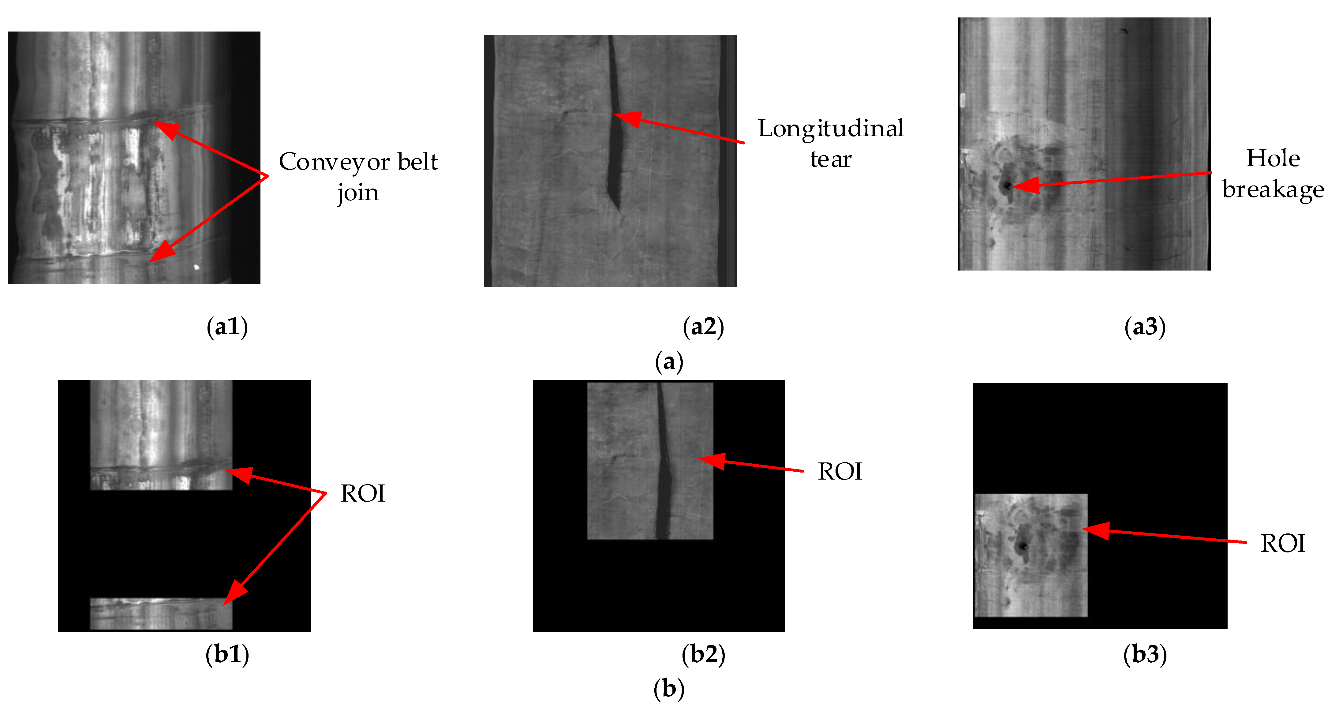
Adaptive partition and block operation. (a) Original image. (a1) Conveyor belt joint image (Image 1). (a2) Longitudinal tear image (Image 2). (a3) Hole breakage image (Image 3). (b) Region of interest (ROI) partition results. (b1) ROI of Image 1. (b2) ROI of Image 2. (b3) ROI of Image 3. (c) Adaptive partition and block operation for Image 1. (c1) Extracted ROI image of Image 1. (c2) Block 1 of Figure 9(c1). (c3) Block 2 of Figure 9(c1). (c4) Extracted ROI image of Image 1. (c5) Block 1 of Figure 9(c4). (c6) Block 2 of Figure 9(c4). (d) Adaptive partition and block operation for Image 2. (d1) Extracted ROI image of Image 2. (d2) Block 1 of Figure 9(d1). (d3) Block 2 of Figure 9(d1). (e) Adaptive partition and block operation for Image 3. (e1) Extracted ROI image of Image 3. (e2) Block 1 of Figure 9(e1). (e3) Block 2 of Figure 9(e1).
Figure 9.
Adaptive partition and block operation. (a) Original image. (a1) Conveyor belt joint image (Image 1). (a2) Longitudinal tear image (Image 2). (a3) Hole breakage image (Image 3). (b) Region of interest (ROI) partition results. (b1) ROI of Image 1. (b2) ROI of Image 2. (b3) ROI of Image 3. (c) Adaptive partition and block operation for Image 1. (c1) Extracted ROI image of Image 1. (c2) Block 1 of Figure 9(c1). (c3) Block 2 of Figure 9(c1). (c4) Extracted ROI image of Image 1. (c5) Block 1 of Figure 9(c4). (c6) Block 2 of Figure 9(c4). (d) Adaptive partition and block operation for Image 2. (d1) Extracted ROI image of Image 2. (d2) Block 1 of Figure 9(d1). (d3) Block 2 of Figure 9(d1). (e) Adaptive partition and block operation for Image 3. (e1) Extracted ROI image of Image 3. (e2) Block 1 of Figure 9(e1). (e3) Block 2 of Figure 9(e1).


Figure 10.
The result of 128 × 128 block for the ROI image extracted in Figure 9(d1). (a) (1,1). (b) (1,2). (c) (1,3). (d) (1,4). (e) (2,1). (f) (2,2). (g) (2,3). (h) (2,4). (i) (3,1). (j) (3,2). (k) (3,3). (l) (3,4). (m) (4,1). (n) (4,2). (o) (4,3). (p) (4,4). (q) (5,1). (r) (5,2). (s) (5,3). (t) (5,4).

Figure 11.
Flow chart of feature-based adaptive partition block registration method.

Figure 12.
Experimental platform.

Figure 13.
Speeded up robust features (SURF) extraction and description. (a) Image 1. (a1) Original image of Image 1. (a2) ROI of Image 1. (a3) Block 1 of Image 1. (a4) Block 2 of Image 1. (a5) Feature points of Figure 13(a1). (a6) Feature points of Figure 13(a2). (a7) Feature points of Figure 13(a3). (a8) Feature points of Figure 13(a4). (b) Image 2. (b1) Original image of Image 2. (b2) ROI of Image 2. (b3) Block 1 of Image 2. (b4) Block 2 of Image 2. (b5) Feature points of Figure 13(b1). (b6) Feature points of Figure 13(b2). (b7) Feature points of Figure 13(b3). (b8) Feature points of Figure 13(b4).


Figure 14.
Random sample consensus (RANSAC) matching of feature points. (a) Figure 13(a5) and Figure 13(b5) registration. (b) Figure 13(a6) and Figure 13(b6) registration. (c) Figure 13(a7) and Figure 13(b7) registration. (d) Figure 13(a8) and Figure 13(b8) registration.

Figure 15.
Application of the proposed research. (a) A mine site. (b) The installed device.

Figure 16.
Stitching effect of AMIM method. (a) Two view image group 1. (a1) Left image. (a2) Right image. (b) Two view image group 2. (b1) Left image. (b2) Right image. (c) Two view image group 1 mosaic image. (d) Two view image group 2 mosaic image.
Figure 16.
Stitching effect of AMIM method. (a) Two view image group 1. (a1) Left image. (a2) Right image. (b) Two view image group 2. (b1) Left image. (b2) Right image. (c) Two view image group 1 mosaic image. (d) Two view image group 2 mosaic image.


Table 1.
Results of the ROI adaptive partition and blocking method.
| Image | ROI | Block 1 | Block 2 | |||||
|---|---|---|---|---|---|---|---|---|
| Number | Size | Blocks Number | Standard Deviation | Position | Standard Deviation | Position | Standard Deviation | |
| Figure 9(a1) | 2 | 896 × 1152 | 9 × 7 | 38.289 | (7,7) | 61.055 | (7,6) | 51.947 |
| 256 × 1152 | 9 × 2 | 28.983 | (1,5) | 35.055 | (1,4) | 32.219 | ||
| Figure 9(a2) | 1 | 640 × 512 | 5 × 4 | 20.741 | (5,3) | 31.456 | (4,3) | 30.289 |
| Figure 9(a3) | 1 | 512 × 512 | 4 × 4 | 32.263 | (2,2) | 39.426 | (1,1) | 32.247 |
Table 2.
Comparison of image feature extraction when the threshold value of Hessian matrix determinant response value is 1000.
Table 2.
Comparison of image feature extraction when the threshold value of Hessian matrix determinant response value is 1000.
| Parameters | Figure 13(a5) | Figure 13(a6) | Figure 13(a7) | Figure 13(a8) | Figure 13(b5) | Figure 13(b6) | Figure 13(b7) | Figure 13(b8) |
|---|---|---|---|---|---|---|---|---|
| Quantity (piece) | 232 | 152 | 16 | 15 | 175 | 122 | 7 | 22 |
| Time (ms) | 578 | 234 | 8 | 8 | 546 | 203 | 8 | 8 |
Table 3.
Comparison of image feature extraction by different threshold values of Hessian matrix determinant response value.
Table 3.
Comparison of image feature extraction by different threshold values of Hessian matrix determinant response value.
| Threshold | Parameters | Figure 13(a5) | Figure 13(a6) | Figure 13(a7) | Figure 13(a8) | Figure 13(b5) | Figure 13(b6) | Figure 13(b7) | Figure 13(b8) |
|---|---|---|---|---|---|---|---|---|---|
| 500 | Quantity (piece) | 694 | 373 | 27 | 35 | 647 | 334 | 29 | 39 |
| Time (ms) | 811 | 265 | 15 | 15 | 733 | 281 | 15 | 15 | |
| 1000 | Quantity (piece) | 232 | 152 | 16 | 15 | 175 | 122 | 7 | 22 |
| Time (ms) | 578 | 234 | 8 | 8 | 546 | 203 | 8 | 8 | |
| 1500 | Quantity (piece) | 114 | 74 | 8 | 11 | 88 | 61 | 5 | 14 |
| Time (ms) | 483 | 125 | 8 | 8 | 437 | 125 | 8 | 8 | |
| 2000 | Quantity (piece) | 64 | 44 | 3 | 10 | 48 | 28 | 1 | 9 |
| Time (ms) | 468 | 125 | 8 | 8 | 406 | 125 | 8 | 8 |
Table 4.
Comparison of the registration.
| Image | Number of Feature Points (Piece) | Registration Number (Pairs) | Registration Time (ms) |
|---|---|---|---|
| Original Image | 407 | 14 | 12 |
| ROI Image | 274 | 10 | 9 |
| Block Image | 60 | 4 | 5 |
Publisher’s Note: MDPI stays neutral with regard to jurisdictional claims in published maps and institutional affiliations. |
© 2021 by the authors. Licensee MDPI, Basel, Switzerland. This article is an open access article distributed under the terms and conditions of the Creative Commons Attribution (CC BY) license (http://creativecommons.org/licenses/by/4.0/).
Share and Cite
MDPI and ACS Style
Gao, R.; Miao, C.; Li, X. Adaptive Multi-View Image Mosaic Method for Conveyor Belt Surface Fault Online Detection. Appl. Sci. 2021, 11, 2564. https://doi.org/10.3390/app11062564
AMA Style
Gao R, Miao C, Li X. Adaptive Multi-View Image Mosaic Method for Conveyor Belt Surface Fault Online Detection. Applied Sciences. 2021; 11(6):2564. https://doi.org/10.3390/app11062564
Chicago/Turabian StyleGao, Rui, Changyun Miao, and Xianguo Li. 2021. "Adaptive Multi-View Image Mosaic Method for Conveyor Belt Surface Fault Online Detection" Applied Sciences 11, no. 6: 2564. https://doi.org/10.3390/app11062564
Note that from the first issue of 2016, this journal uses article numbers instead of page numbers. See further details here.