Mesh-Free Surrogate Models for Structural Mechanic FEM Simulation: A Comparative Study of Approaches

Abstract

The technical world of today fundamentally relies on structural analysis in the form of design and structural mechanic simulations. A traditional and robust simulation method is the physics-based finite element method (FEM) simulation. FEM simulations in structural mechanics are known to be very accurate; however, the higher the desired resolution, the more computational effort is required. Surrogate modeling provides a robust approach to address this drawback. Nonetheless, finding the right surrogate model and its hyperparameters for a specific use case is not a straightforward process. In this paper, we discuss and compare several classes of mesh-free surrogate models based on traditional and thriving machine learning (ML) and deep learning (DL) methods. We show that relatively simple algorithms (such as k-nearest neighbor regression) can be competitive in applications with low geometrical complexity and extrapolation requirements. With respect to tasks exhibiting higher geometric complexity, our results show that recent DL methods at the forefront of literature (such as physics-informed neural networks) are complicated to train and to parameterize and thus, require further research before they can be put to practical use. In contrast, we show that already well-researched DL methods, such as the multi-layer perceptron, are superior with respect to interpolation use cases and can be easily trained with available tools. With our work, we thus present a basis for the selection and practical implementation of surrogate models.

1. Introduction

Assessing the properties of mechanical structures with real physical experiments is expensive, as it costs both time and resources. To reduce these costs of knowledge enrichment in the field of structural analysis, computer simulations of structural mechanics have become crucial. An essential simulation method is the finite element method (FEM) in which the simulation domain space is represented by a finite number of connected elements. Space- and time-dependent behavior between connected elements and within the elements themselves is governed by physical equations. Observation of real physical experiments provides the coefficients for these governing equations. Since most geometries and use cases cannot be solved analytically, an approximation of the proposed physical equations is obtained by numerical methods [1]. However, solving complex problems with FEM is time-consuming and computationally expensive. In order to reduce the computational effort, surrogate modeling offers a promising solution [2].

Surrogate models are trained in a supervised manner and are designed to learn the function mapping between inputs and outputs from a given FEM simulation use case. With a sufficient amount of training data with respect to the use case, an according model is able to substitute for the FEM simulation use case up to a certain accuracy.

There is already a considerable number of related work concerning surrogate modeling of structural mechanics simulations with machine learning (ML) or deep learning (DL) approaches. In the following, we want to present the most important works for this paper. Artificial neural networks (ANN) are used in the work of Roberts et al. [3] to predict damage development in forged brake discs reinforced with Al-SiC particles, using damage maps. The ANN is a multilayer perceptron (MLP), and training data are obtained from FEM simulations using the commercial DEFORM simulation software. For rapid estimation of forming and cutting forces for given process parameters, Hans Raj et al. [4] investigate a method using MLP models. The researchers focus on two processes: hot upsetting and extrusion. Each process, represented by a MLP, is trained with FEM simulation results from the FORGE2 commercial FEM simulation software. García-Crespo et al. [5] predict the projectile response after impact with steel armor using a MLP; their surrogate model studied is trained with data from FEM simulations of the use case. Nourbakhsh et al. [6] explore generalizable surrogate models for 3D trusses, using MLP and FEM training data. Chan et al. [7] estimate the performance of hot-forged product designs, using a MLP trained on FEM results obtained with the commercial software DEFORM. D’Addona and Antonelli [8] use single-layer feedforward ANNs instead of FEM as a metamodel in a sequential approximate optimization (SAO) algorithm. In a case study on hot forging of a steel disk, they compare their results with an ANN trained on FEM simulation results and the FEM simulation software QForm3D. Gudur and Dixit [9] predict the velocity field and location of neutral point of cold flat rolling with a MLP trained with rigid-plastic FEM simulation results. Pellicer-Valero et al. [10] predict the mechanical behavior of different livers with MLPs trained from FEM simulations.

Abueidda et al. [11] estimate the mechanical properties of a two-dimensional checkerboard composite using a convolutional neural network (CNN) trained with FEM results. Regarding mesh-based approaches, Pfaff et al. [12] present a framework to train graph neural networks (GNN) on mesh-based simulations and show the applicability in aerodynamics, structural mechanics, and fabric.

Surrogate models were also obtained using classical, i.e., non-neural ML, approaches. For example, the authors of [3] apply Gaussian process regression (GPR) besides ANN in their approach. Loghin and Ismonov [13] predict the stress intensity factors, using GPR trained with FEM results of a classical bolt-nut assembly. Ming et al. [14] model the electrical discharge machining process with GPR trained from data generated with numerical FEM simulation.

Using support vector regression (SVR), Pan et al. [15] construct a metamodel in an optimization approach for lightweight vehicle design. Training data are generated, using design of experiment approaches with FEM simulations. To predict the stress at the implant–bone interface, Li et al. [16] utilize SVR in order to replace FEM simulation. Hu and Li [17] estimate cutting coefficients in a mechanistic milling force model with SVR trained with FEM simulation data.

Employing tree-based models, Martínez-Martínez et al. [18] estimate the biomechanical behavior of breast tissue under compression, using three different tree-based models trained from FEM simulations. The models are trained with FEM data in terms of nodal coordinates and nodal tissue membership. Zhang et al. [19] estimate the base failure stability for braced excavations in anisotropic clay using extreme gradient boosting, random forest regression (RFR) and data obtained from FEM simulation results. Qi et al. [20] utilize a decision tree regressor to predict the mechanical properties of carbon fiber reinforced plastics with data obtained from FEM simulations. Besides MLPs Pellicer-Valero et al. [10] utilize RFRs to predict the biomechanics of livers.

A recent neural network–based approach are physics informed neural networks (PINNs). PINNs are trained simultaneously on data and governing differential equations and can be used for the solution and inversion of equations governing physical systems. Utilizing PINNs, Haghighat and Juanes [21] substitute a particular FEM simulation of a perforated strip under uniaxial extension. In [22], Haghighat et al. present a surrogate modeling approach with PINNs and a specific use case. Focusing on consistency, Shin [23] evaluates findings regarding PINNs with Poisson’s equation and the heat equation. Yin et al. [24] use PINNs to predict permeability and viscoelastic modulus from thrombus deformation data, described by the fourth-order Cahn–Hilliard and Navier–Stokes equations. In addition to the application of PINNs in structural mechanics problems, there is also a considerable number of papers, especially in computational fluid dynamics [25,26,27,28,29].

Related work shows capabilities of surrogate modeling, thus demonstrating the feasibility of supervised learning models trained with FEM simulations. From our analysis of the existing literature, we identify the following drawbacks:

• In most cases, the surrogate model only substitutes for a subset of the considered computational domain. Thus, such an approach focuses only on a region of interest and cannot be used to evaluate the entire computational domain (notable exceptions are [12,22]).
• Surrogate models representing the complete discretized computational domain (mesh) are solely fitted and evaluated on one use case—generalization to unseen data is only achieved with respect to the discretization of the computational domain, but not with respect to other use case specific parameters (notable exception concerning material parameters [22]).
• Due to differences in FEM use cases and data, the comparison of related work is useful only in some cases.
• Replication of published experiments is often not achievable because important parameters are not reported, e.g., number of finite elements, type of finite elements (bilinear, biquadratic, reduced integration etc.), method of discretization (meshing), as well as hyperparameters of the ML models, such as learning or activation functions.

To address these drawbacks, we present the following contributions of our paper:

• We present the main DL and ML methods together with a compact description and mathematical notation to equip practitioners with a reference to surrogate FEM simulation mesh-free and assess the feasibility and maturity of the novel PINNs method.
• We utilize three classic use cases in structural mechanics and evaluate these models in terms of performance on unseen configurations (inter- and extrapolation) in order to assess their ability to generalize across different use case specific parameters.
• We discuss the characteristics of all DL and ML models, and their practical implications, in the context of the use cases.

With our work, we pave the way of mesh-free surrogate modeling for practical use: we provide a basis for efficient model and hyperparameters selection regarding use case and performance metrics. These insights shall not only assist the domain expert during model selection, but will also help in consolidating the current research in mesh-free surrogate modeling for structural mechanics applications.

We report all information to make our experiments reproducible. If certain model settings are not mentioned, they are left at default values. Moreover, our FEM simulations are performed with Abaqus Student Edition 2019 (Dassault Systèmes, Velizy-Villacoublay, France), and thus, the process of data generation is not limited to commercial software, which makes it possible for everyone to connect to our research.

The remainder of this paper is organized as follows. In Section 2, we present the materials and methods of our experiments, first providing insights into the process of data generation, using the FEM simulations in Section 2.1, then describing the datasets obtained from the FEM simulations in Section 2.2, followed by the ML and DL models used in Section 2.3. Section 3 shows the results, which are discussed in Section 4. In Section 5, we present the conclusion of our work and an outlook for the future.

2. Materials and Methods

In this section, we present all relevant information about the methodology of our experiments. First, Section 2.1 provides an overview of the data generation process, using three classic FEM simulation use cases. Then, Section 2.2 describes the datasets used from the FEM simulations, and Section 2.3 presents the ML and DL models used. A more detailed overview of the mathematical background and assumptions of the ML and DL models can be found in the Appendix. When predicting a particular use case with a surrogate model, the individual nodes discretizing the particular geometry of the use case (i.e., mesh) are sequentially input into the surrogate model with the appropriate generalization variable. The surrogate model then predicts the output of each node in sequence; see Figure 1.

It should be noted that there are no constraints on the discretization (mesh), i.e., the node coordinates can be freely chosen within the simulation domain and nodes are not connected to each other. Therefore, we refer to our approach as mesh-free, but we want to clearly distinguish ourselves from other mesh-free methods, such as smoothed particle hydrodynamics, the diffuse element method, the moving particle finite element method, etc. The predictions of the individual nodes together constitute the prediction for the simulation domain of the particular use case. By adding the nodal displacement outputs of the surrogate model to the initial node coordinates, we obtain the new deformed geometry. Further surrogate model outputs (e.g., stresses, strains) describe the queried nodes and thus the complete simulation domain in more detail.

2.1. FEM Use Cases

For illustration, we base our evaluation on three classic use cases from structural mechanics. We consider the (1) tensile load, (2) bending load and (3) compressive load:

• Elongation of a plate with a perforation;
• Bending of a beam;
• Compression of a block with four perforations.

See

Table 1. Classic FEM use cases. Overview of the three use cases and their main change and types of deformations. In the first two use cases, only a single change is conduced, while in the last use case, a combination of changes is studied.

Use Case	Change	Deformation
Plate	Geometry	Elongation
Beam	Material Properties	Bending
Block	Geometry, Material Properties	Compression

and Figure 2. We utilize an isotropic elasto-plastic rate-independent material model (i.e., a perfectly plastic material). The kinematic relations for our 2D plane strain use cases are defined by the total strain components ${\epsilon }_{xx}=\frac{\partial u_x}{\partial x}$, ${\epsilon }_{yy}=\frac{\partial u_y}{\partial y}$, ${\epsilon }_{xy}=\frac{1}{2}(\frac{\partial u_x}{\partial y}+\frac{\partial u_y}{\partial x})$, ${\epsilon }_{zz}=0$ with displacements $u_x$ and $u_y$ and deviatoric strain components $e_{xx}={\epsilon }_{xx}-\frac{{\epsilon }_{vol}}{3}$, $e_{yy}={\epsilon }_{yy}-\frac{{\epsilon }_{vol}}{3}$, $e_{xy}={\epsilon }_{xy}$ and $e_{zz}=-\frac{{\epsilon }_{vol}}{3}$. Since there is no volumetric plastic strain in the von Mises yield function, the volumetric strain can be expressed as ${\epsilon }_{vol}=\mathrm{trace}\left(\epsilon \right)$ s.t. ${\epsilon }_{vol}={\epsilon }_{xx}+{\epsilon }_{yy}$. The deviatoric stress components are defined by $s_{xx}={\sigma }_{xx}-\left(\frac{{\sigma }_{xx}+{\sigma }_{yy}+{\sigma }_{zz}}{3}\right)$, $s_{yy}={\sigma }_{yy}-\left(\frac{{\sigma }_{xx}+{\sigma }_{yy}+{\sigma }_{zz}}{3}\right)$, $s_{xy}={\sigma }_{xy}$ and $s_{zz}={\sigma }_{zz}-\left(\frac{{\sigma }_{xx}+{\sigma }_{yy}+{\sigma }_{zz}}{3}\right)$, where ${\sigma }_{ij}$ ($i,j\in \left\{x,y\right\}$) are the components of the Cauchy stress tensor. The plastic strain components are defined by ${\epsilon }_{xx}^{pl}={\overline{\epsilon }}^{pl}\frac{3}{2}\frac{s_{xx}}{q}$, ${\epsilon }_{yy}^{pl}={\overline{\epsilon }}^{pl}\frac{3}{2}\frac{s_{yy}}{q}$, ${\epsilon }_{xy}^{pl}={\overline{\epsilon }}^{pl}\frac{3}{2}\frac{s_{xy}}{q}$ and ${\epsilon }_{zz}^{pl}={\overline{\epsilon }}^{pl}\frac{3}{2}\frac{s_{zz}}{q}$ with equivalent plastic strain of the von Mises model as ${\overline{\epsilon }}^{pl}=\overline{\epsilon }-\frac{{\sigma }_Y}{3\mu }\ge 0$, where ${\sigma }_Y$ is the yield stress and $\mu$ the second Lamé parameter. The total equivalent strain is defined by $\overline{\epsilon }=\sqrt{\frac{2}{3}{\sum }_{i,j\in \left\{x,y\right\}}{e}_{ij}{e}_{ij}}$ with deviatoric strain components $e_{ij}$. The decomposition of the strain is ${\epsilon }_{ij}={\epsilon }_{ij}^{el}+{\epsilon }_{ij}^{pl}$ with elastic component ${\epsilon }_{ij}^{el}$ and plastic component ${\epsilon }_{ij}^{pl}$ of the respective strain matrices. The equivalent stress is defined by $q=\sqrt{\frac{3}{2}{s}_{ij}{s}_{ij}}$. In our PINN approach, we utilize the definitions of the total strain components, deviatoric strain and stress components and plastic strain components in the respective regularization term.

We use quarter symmetry in use cases 1 and 3 to make efficient use of computational resources. Additional information regarding the variation of parameters in the simulations is presented in

Table 2. Dataset generation by executing several different simulations with varying generalization variables (Plate: perforation $Diameter$, Beam: $YieldStress$ and Block: $YieldStress$ and $Width$), bold marked simulations are not in the training dataset and only used for test and evaluation. Interpolation tasks are marked with superscript $\left(i\right)$ and extrapolation tasks with superscript $\left(e\right)$.

Plate
Simulation ID	1 ${}^{\left(\mathit{e}\right)}$	2	3	4 ${}^{\left(\mathit{i}\right)}$	5	6 ${}^{\left(\mathit{i}\right)}$	7	8	9 ${}^{\left(\mathit{e}\right)}$
Diameter [mm]	60	70	80	90	100	110	120	130	140
Beam
Simulation ID	1 ${}^{\left(\mathit{e}\right)}$	2	3	4 ${}^{\left(\mathit{i}\right)}$	5	6 ${}^{\left(\mathit{i}\right)}$	7	8	9 ${}^{\left(\mathit{e}\right)}$
Yield Stress [MPa]	850	900	950	1000	1050	1100	1150	1200	1250
Block
Simulation ID	1 ${}^{\left(\mathit{e}\right)}$	2 ${}^{\left(\mathit{e}\right)}$	3	4	5	6	7 ${}^{\left(\mathit{i}\right)}$	8	9	10	11	12 ${}^{\left(\mathit{e}\right)}$	13 ${}^{\left(\mathit{e}\right)}$
Yield Stress [MPa]	750	750	900	900	900	1050	1050	1050	1200	1200	1200	1350	1350
Width [mm]	180	260	200	220	240	200	220	240	200	220	240	180	260

, where simulations marked in bold are used for the test and evaluation of the surrogate models and are not in the training dataset. Conversely, simulations not marked in bold represent the training dataset and are not in the test dataset. In use cases exhibiting varied geometry parameters (i.e., elongation of a plate and compression of a block use cases), the mesh is also different in each simulation. Thus, we train and evaluate the surrogate models on use cases with different meshes (i.e., in each simulation, the node coordinates differ).

The first use case, a perforated steel strip under tensile load, is similar to the nonlinear solid mechanics use case of [21,22]. However, in our approach, we evaluate the generalization over the perforation diameter and use material properties for steel and a top edge displacement of 5 mm in positive y-axis to consider a more challenging use case.

We execute different simulation settings, where the generalization variable (diameter of perforation) is changed in each simulation; see Figure 2a and Table 2. In our second use case, we simulate a bending beam that end is displaced about 5 mm in the positive x-direction; see Figure 2b. We vary the yield stress generalization variable in each simulation setting; see Table 2. In our third use case, we simulate a quarter-symmetric block with four perforations under compressive load, which is compressed about 5 mm in the negative y-axis; see Figure 2c. In this use case, we vary two generalization variables (yield stress and width of the block) in each simulation; see Table 2.

We evaluate our models on interpolation (i.e., that the generalization variables for testing are within the range of the generalization variables observed during training) and extrapolation (i.e., that the generalization variables for testing are outside the range of the generalization variables observed during training) tasks. In Table 2, we mark interpolation tasks with superscript $\left(i\right)$ and extrapolation tasks with superscript $\left(e\right)$.

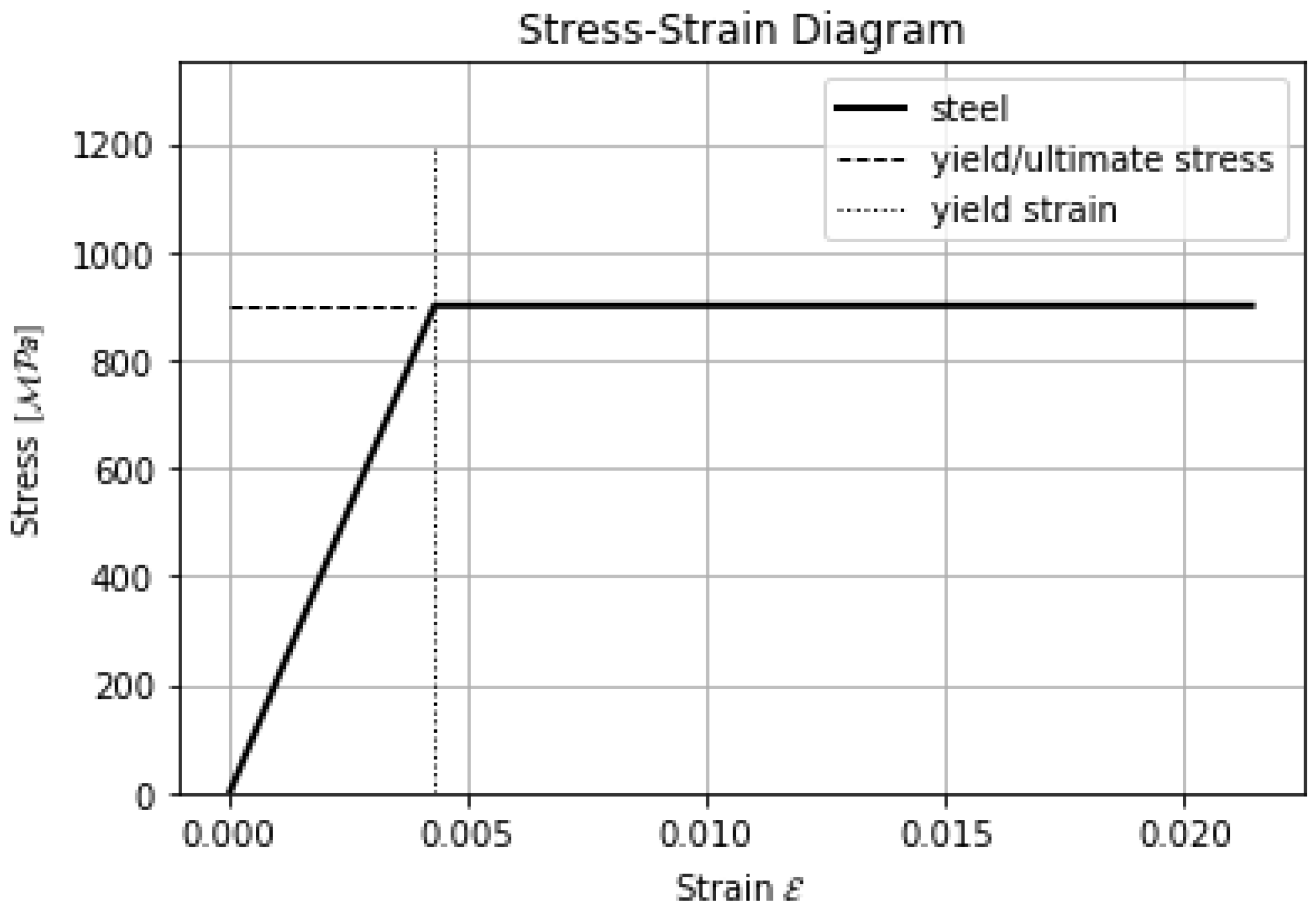
In Figure 3, we present the perfect nonlinear elastoplastic material behavior of our use cases. The Young’s modulus is 210 GPa, Poisson’s ratio 0.3 and the yield stress 900 MPa. In our first use case, the perforated plate, we use this setting in each simulation. In the other two use cases, the yield stress varies, while the remaining material parameters stay the same.

All parts are meshed, using plane strain 4-node bilinear quadrilateral elements with reduced integration and hourglass control. Please note that although [22] recommends the use of larger order elements for the approximation of body forces, we use bilinear elements since we do not use body forces in our surrogate modeling approaches. We create a finer mesh near additional geometric details (i.e., perforations in the plate and block use cases) and seed the perforation edge of the plate with an approximate size of 3.8 mm and the remaining edges with an approximate size of 5 mm. The perforation edges of the block are seeded with an approximate size of 3 mm and the remaining edges with an approximate size of 4 mm. The beam exhibits no comparable geometric details; thus, we seed all edges with an approximate size of 1.5 mm.

We obtain our FEM simulation results in the context of general static simulations. Details of the simulation steps are shown in

Table 3. Abaqus FEM simulation control parameters.

Abaqus FEM Simulation Settings
Simulation type	Static, General
Time period	1
Nlgeom	On
Max number of increments	100
Initial increment size	1
Min increment size	1 × 10−5
Max increment size	1
Equation solver method	Direct
Solution technique	Full Newton

. Simulation control parameters that are not listed are left at default values.

2.2. Dataset

The nodal data from our Abaqus FEM simulations constitute the datasets. For each use case, the nodal data are split into training and test dataset, respectively. The training dataset $D=\left\{X_1,\dots ,X_n\right\}$ with number of training instances n and the test dataset $T=\left\{X_{n+1},\dots ,X_{n+m}\right\}$ with number of test instances m are generated from several FEM simulations; see Table 2 and

Table 6. Dataset splits: number of training instances n and test instances m due to the data generation from Table 2.

	Plate	Beam	Block
Training dataset D	4447	2720	6722
Test dataset T	3534	2176	4107

, where bold marked simulations belong to T and the remaining to D. Thus, we split our data due to different generalization variables and not randomly. We denote each instance with index i, $i\in \{1,2,\cdots ,n+m\}$. An instance $X_i=(x_i,y_i)$ is generated of an input vector $x_i\in {\mathbb{R}}^p$ and output vector $y_i\in {\mathbb{R}}^q$. Each input vector $x_i$ is composed of the initial x- and y-coordinates of a FEM node and the respective generalization variable (i.e., perforated plate: $Diameter$, beam: $YieldStress$, block with four perforations: $Width$ and $YieldStress$) of the FEM simulation; see

Table 4. Surrogate model input variables. Data obtained from FEM simulations are transformed so that each FEM node (represented by its x- and y-coordinates) with the respective generalization variable is an instance.

Simulation	Plate	Beam	Block
Input variables	x-coordinate	x-coordinate	x-coordinate
	y-coordinate	y-coordinate	y-coordinate
	Diameter	Yield Stress	Yield Stress
			Width

. Thus, we have $p=3$ in the plate and beam use case, and $p=4$ in the block use case.

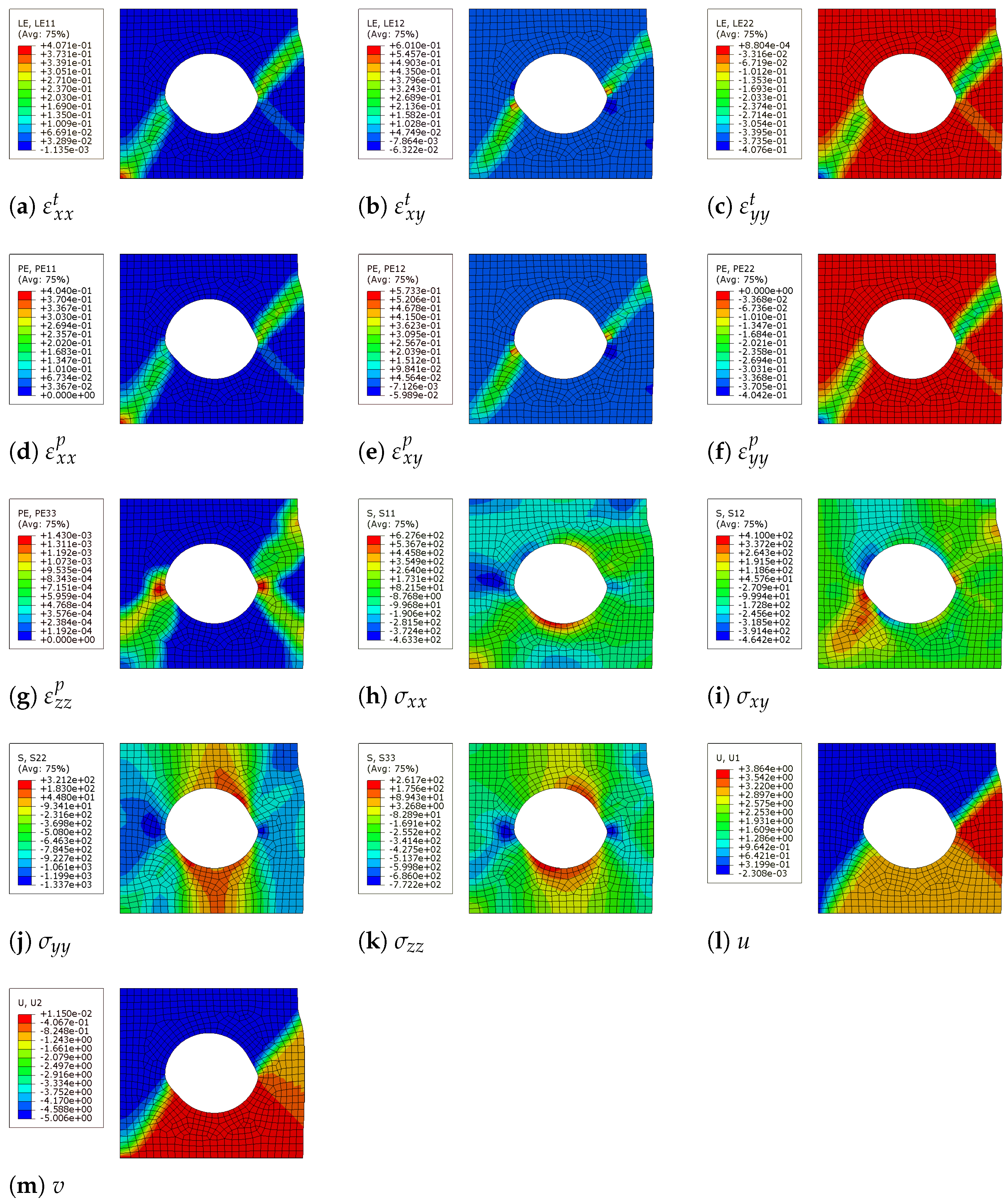
In our setting, each output vector $y_i$ contains 13 ($q=13$) output variables obtained from FEM simulation with input $x_i$, namely the ${\epsilon }_{xx}^t$, ${\epsilon }_{xy}^t$ and ${\epsilon }_{yy}^t$ total strain components, the ${\epsilon }_{xx}^p$, ${\epsilon }_{xy}^p$, ${\epsilon }_{yy}^p$ and ${\epsilon }_{zz}^p$ plastic strain components, the ${\sigma }_{xx}$, ${\sigma }_{xy}$, ${\sigma }_{yy}$ and ${\sigma }_{zz}$ principal and shear stress components and the displacement in x- and y-directions u and v of each node; see

Table 5. Surrogate model output variables. For each input FEM node, a surrogate model predicts its respective strains, stresses and displacements.

Output Variables
${\epsilon }_{xx}^t$	${\epsilon }_{xx}^p$	${\sigma }_{xx}$	u
${\epsilon }_{xy}^t$	${\epsilon }_{xy}^p$	${\sigma }_{xy}$	v
${\epsilon }_{yy}^t$	${\epsilon }_{yy}^p$	${\sigma }_{yy}$
	${\epsilon }_{zz}^p$	${\sigma }_{zz}$

and Figure 4. We split the data in a training and test dataset (see Table 6) and standardized the data by removing the mean and scaling to unit variance.

In Figure 4, we present graphical results with visible mesh obtained from Abaqus FEM simulation of the output variables used for a block use case.

2.3. Surrogate Models

In this section, we give an overview of the surrogate models used and their general assumptions; to highlight the differences as well as the advantages and disadvantages between them, we present a detailed mathematical background in Appendix A. We have selected models from different learning paradigms:

• Gradient boosting decision tree regressor (GBDTR): piecewise constant model.
• K-nearest neighbor regressor (KNNR): distance-based model.
• Gaussian process regressor (GPR): Bayesian model.
• Support vector regressor (SVR): hyperplane-based model.
• Multi layer perceptron (MLP): classic feedforward neural network model.
• Physics informed neural network (PINN): neural network model with physics-based regularization.

3. Results

For evaluation, we split the data into a training and test dataset to fit and test our surrogate models; see Table 6 for the dataset sizes and Table 2 for more details regarding the data split.

As a next step, we need to define hyperparameters for each model and each use case. We performed hyperparameter optimization using only training data; no test data were used. In our PINN approaches, the adaptation of hyperparameters was based on the work of [21,22]. Our MLPs were designed to be similar to our PINNs to allow for fair comparisons. We varied hyperparameters in our neural network approaches (MLP and PINN) following best practices and guidelines, where we optimized the number of hidden layers, number of neurons per hidden layer, activation function, validation split, earlystopping patience and the size of the batch per training epoch. Regarding the rest of our models, we applied a grid-search with a five fold cross-validation, utilizing the training data to obtain the best hyperparameters. The hyperparameters for each use case are in Appendix B and

Table A1. Best performing hyperparameters GBDTR.

	Plate	Beam	Block
loss	ls	ls	ls
criterion	friedman_mse	mse	friedman_mse
max_features	auto	log2	auto
n_estimators	400	1000	2000

,

Table A2. Best performing hyperparameters KNNR.

	Plate	Beam	Block
n_neighbors (K)	7	5	10
weights	distance	distance	distance
algorithm	brute	ball_tree	auto
leaf_size	1	5	1
p_value	1	2	5

,

Table A3. Best performing hyperparameters GPR.

	Plate	Beam	Block
kernel	Matern()**2	RationalQuadratic()**2	RationalQuadratic()**2
alpha	10−13	10−13	10−14

,

Table A4. Best performing hyperparameters SVR.

	Plate	Beam	Block
kernel	rbf	rbf	rbf
gamma	scale	scale	scale
epsilon	0.005	0.005	0.4
C	95	5	105

,

Table A5. Best performing hyperparameters MLP.

	Plate	Beam	Block
hidden layers	3	2	4
neurons	100-100-100	100-100	100-100-100-100
activation function	relu	relu	relu
batch size	32	32	64
validation split	0.1	0.1	0.1
early stopping patience	5000	5000	7500
max epochs	100,000	100,000	100,000
stopped at	27,693	26,383	43,272

and

Table A6. Best hyperparameters PINN.

	Plate	Beam	Block
hidden layers	4	4	4
neurons	100-100-100-100	100-100-100-100	100-100-100-100
activation function	tanh	tanh	tanh
batch size	64	64	64
epochs	50,000	50,000	50,000

.

Our evaluation is based on R2-scores with respect to the FEM results and inference time. For models that contain inherent randomness, such as MLPs, GBDTR and PINNs, a five-fold cross-validation was conducted. For these models, we report the mean values and standard deviation of the R2-score. For the sake of brevity, we report only the average R2-scores across all 13 targets in this section; see

Table 7. Plate: averaged results, bold values indicate the best performing surrogate models. Values in parentheses are the corresponding standard deviations of the average R2-scores due to repeated experiments of stochastic process models. For further information concerning simulations, see Table 2.

Model	MLP	PINN	SVR	GBDTR	KNNR	GPR	FEM
	Simulation 1
R2	0.9900 (6.155 × 10−9 )	0.7797 (8.709 × 10−2)	0.6188	0.6606 (3.959 × 10−8 )	0.8164	0.6131	-
Inference time [s]	0.0523	0.0746	1.15	0.311	0.00722	0.151	9.01
	Simulation 4
R2	0.9978 (1.970 × 10−4)	0.9089 (2.598 × 10−2)	0.7174	0.9014 (6.310 × 10−2)	0.9298	0.8761	-
Inference time [s]	0.0781	0.0638	1.20	0.271	0.00734	0.139	9.08
	Simulation 6
R2	0.9920 (1.889 × 10−3 )	0.8470 (6.309 × 10−2 )	0.7251	0.8503 (1.005 × 10−1 )	0.9219	0.8676	-
Inference time [s]	0.0595	0.0641	1.10	0.251	0.00797	0.131	9.88
	Simulation 9
R2	0.9786 (2.970 × 10−5 )	0.7562 (1.046 × 10−1 )	0.6568	0.7263 (9.780 × 10−9 )	0.8045	0.5651	-
Inference time [s]	0.0665	0.0715	1.02	0.251	0.00734	0.139	10.03

,

Table 8. Beam: averaged results, bold values indicate the best performing surrogate models. Values in parentheses are the corresponding standard deviations of the average R2-scores due to repeated experiments of stochastic process models. For further information concerning simulations, see Table 2.

Model	MLP	PINN	SVR	GBDTR	KNNR	GPR	FEM
	Simulation 1
R2	0.6682 (7.345 × 10−6 )	0.6165 (1.648 × 10−2 )	0.5122	0.7120 (1.088 × 10−8 )	0.6288	0.5377	-
Inference time [s]	0.0781	0.0638	1.20	0.271	0.00734	0.139	9.08
	Simulation 4
R2	0.9979 (1.319 × 10−3 )	0.9379 (1.042 × 10−3 )	0.7558	0.9640 (6.751 × 10−4 )	0.9621	0.8243	-
Inference time [s]	0.0457	0.110	0.418	0.0541	0.0790	0.221	6.81
	Simulation 6
R2	0.9981 (8.315 × 10−4 )	0.9314 (8.396 × 10−4 )	0.7406	0.9516 (1.368 × 10−4 )	0.9617	0.8059	-
Inference time [s]	0.0442	0.0668	0.402	0.0569	0.0705	0.212	6.61
	Simulation 9
R2	−1196.2920 (6.166 × 103 )	−1305.9226 (3.269 × 101 )	−107.7646	−830.8926 (4.2984 )	−322.4940	−420.9029	-
Inference time [s]	0.0781	0.0638	1.20	0.271	0.00734	0.139	9.08

and

Table 9. Block: averaged results, bold values indicate the best performing surrogate models. Values in parentheses are the corresponding standard deviations of the average R2-scores, due to repeated experiments of stochastic process models. For further information concerning simulations, see Table 2.

Model	MLP	PINN	SVR	GBDTR	KNNR	GPR	FEM
	Simulation 1
R2	0.5562 (1.952 × 10−1)	−0.4441 (6.066 × 10−1 )	−0.2463	0.5695 (1.665 × 10−3 )	0.7808	0.1059	-
Inference time [s]	0.0781	0.0638	1.20	0.271	0.00734	0.139	9.08
	Simulation 2
R2	0.3768 (3.803 × 10−1 )	0.1850 (5.531 × 10−2 )	−0.1800	0.5149 (3.320 × 10−4 )	0.7366	0.1409	-
Inference time [s]	0.0457	0.110	0.418	0.0541	0.0790	0.221	6.81
	Simulation 7
R2	0.9976 (8.258 × 10−5 )	0.9410 (4.310 × 10−3 )	0.6415	0.9702 (1.884 × 10−2 )	0.9767	0.5200	-
Inference time [s]	0.0442	0.0668	0.402	0.0569	0.0705	0.212	6.61
	Simulation 12
R2	0.6303 (3.204 × 10−1 )	−0.4480 (6.652 × 10−1 )	−0.2230	0.5702 (6.266 × 10−4 )	0.7797	0.1553	-
Inference time [s]	0.0442	0.0668	0.402	0.0569	0.0705	0.212	6.61
	Simulation 13
R2	0.6475 (3.326 × 10−1 )	−0.1122 (3.265 × 10−1 )	−0.0745	0.5894 (1.579 × 10−4 )	0.7687	0.1771	-
Inference time [s]	0.0781	0.0638	1.20	0.271	0.00734	0.139	9.08

. The R2-scores for individual targets are provided in Appendix C. The inference times are based on the mean value of three measurements. Inferences were run on a machine with 16 GB RAM, 8 CPUs and Intel(R) i7-8565 2.0GHz processor. To compare the inference time of our surrogate models with the computation time required to run FEM simulations, we have included the latter also in Table 7, Table 8 and Table 9.

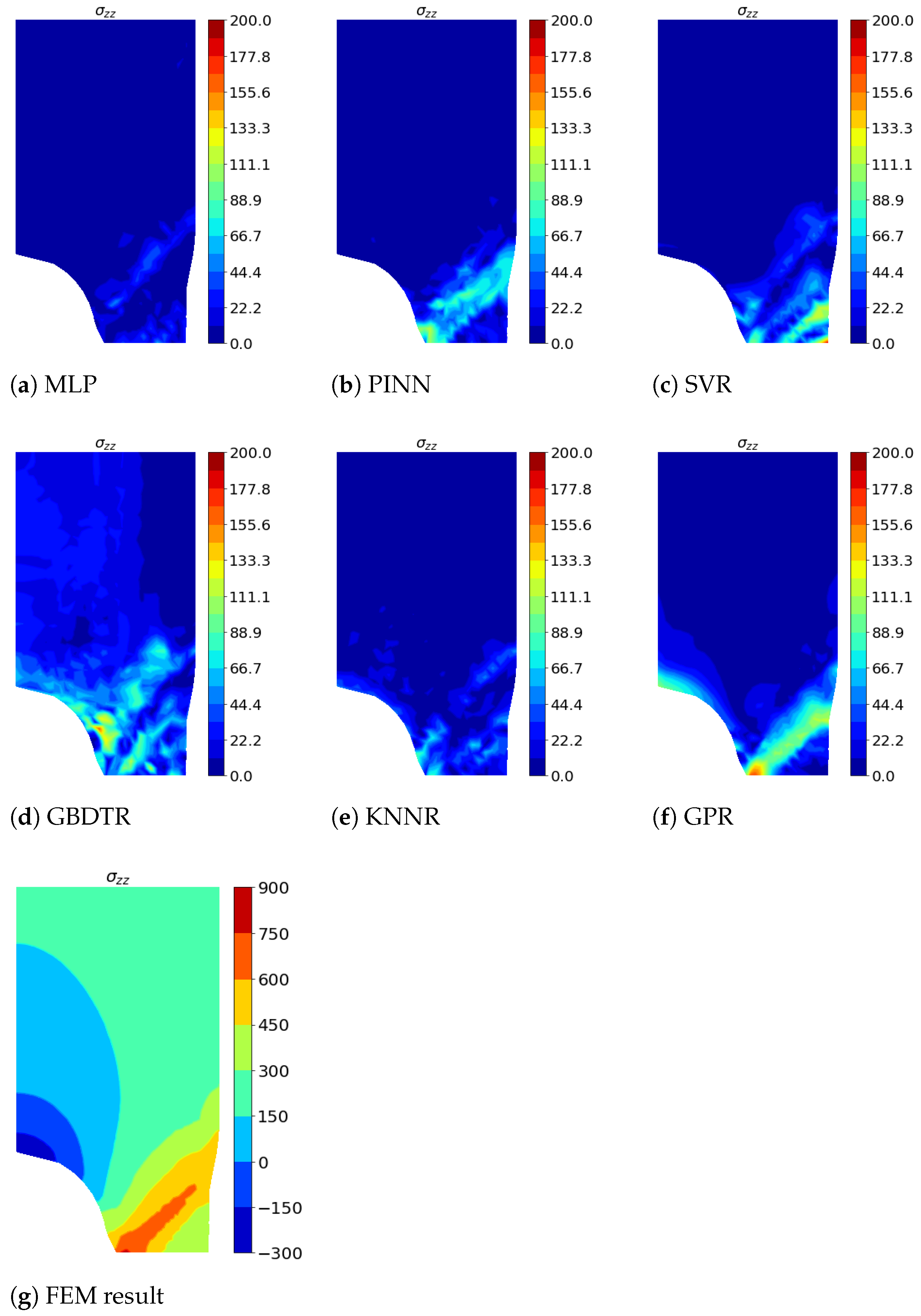
For graphical results, we chose simulations that cover the error situation quite well in order to make statements about the performance of each model. In addition to the absolute errors (Figure 5a–f, Figure 6a–f, Figure 7a–f, Figure 8a–f, Figure 9a–f and Figure 10a–f), the corresponding FEM simulations of the basis are shown in Figure 5g, Figure 6g, Figure 7g, Figure 8g, Figure 9g and Figure 10g.

GBDTR, KNNR, GPR and SVR algorithms were implemented with the scikit-learn library version 0.24.0 in Python. The SVR and GBDTR algorithms were constructed with MultiOutputRegressor scikit-learn API to fit one regressor per target. Regarding our DL algorithms, the utilized MLPs were implemented with the keras API version 2.4.3 and our PINNs were implemented with the sciann API version 0.5.5.0 in Python 3.8.5. We used the PDEs from [21,22], but instead of the inversion part, we trained our PINNs additionally with plastic strain data, same as for the rest of the surrogate models.

In the elongation of a perforated plate use case, our approach is based on a total of nine FEM simulations. We used five simulations for training and four simulations to evaluate the fitted models; see Table 2. We report the average of R2-scores across all outputs in Table 7 with the corresponding inference times.

Regarding extrapolation, the absolute errors of each surrogate model with respect to ${\sigma }_{xy}$ of Simulation 1 are shown in Figure 5. We plot the absolute errors of each surrogate model of ${\sigma }_{zz}$ of Simulation 4 in Figure 6 as an example of interpolation. In addition, we show in both figures the ground truth of the corresponding output variable obtained from the FEM simulation. For both interpolation and extrapolation, the errors are large near the shear band. As far as extrapolation is concerned, in addition to the errors near the shear band, most models have significant errors near the maximum negative xy shear stresses; see blue areas in Figure 5g. GBDTR performs well overall, though the error increases in various locations; while PINNs have a similar average performance, they perform better outside the shear band regarding absolute errors. MLP overall shows the best results followed by KNNR.

In the bending beam use case, similar to the perforated plate use case, we trained our models on five simulations and tested them using the remaining four, see Table 2. We present the average R2-scores across all outputs and inference times in Table 8 for the test simulations 1, 4, 6 and 9.

We provide a graphical representation of the absolute error of the surrogate models regarding ${\epsilon }_{yy}^t$ in Figure 7a–f with the FEM simulation result in (g) as one instance of interpolation. Absolute errors of the surrogate models regarding ${\epsilon }_{xx}^p$ and extrapolation are shown in Figure 8. Overall higher errors can be observed near the encastred boundary condition of the beam for some models for that output. While the PINN shows a competitive average R2-score regarding interpolation, on this single target, its performance shows significant weaknesses.

The compression of a block with four perforations use case presents a more complex setting because we generalize by two generalization variables (yield stress and block width). Therefore, we utilize more training data for this use case; see Table 2. We report the average results of R2-scores with corresponding standard deviations, if applicable, in Table 9.

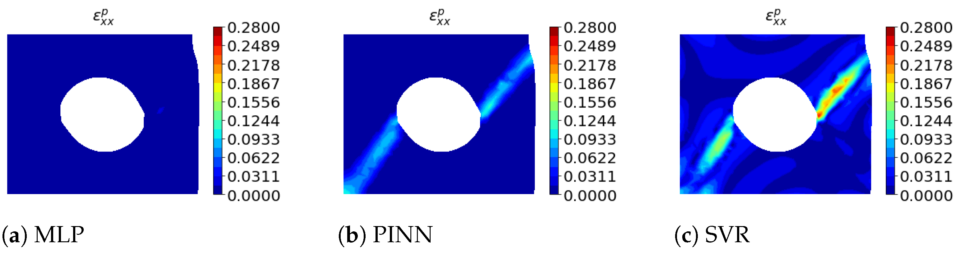
As an instance for interpolation, the absolute errors regarding ${\epsilon }_{xx}^p$ can be seen in Figure 9a–f with Abaqus FEM simulation result (g). Respectively, an instance for extrapolation is shown in Figure 10 with absolute errors (a–f) and FEM ground truth (g). Some models show higher prediction errors near shear bands (high ${\epsilon }_{xx}^p$ regions) regarding the interpolation task. However, SVR and GPR cannot extract meaningful information from the training data, especially in the space free of plastic deformation. This is indicated by the low average R2-scores, compared to the other models. Considering absolute errors of ${\sigma }_{xy}$ and extrapolation the MLP, which is otherwise performing well, shows weaknesses and is in general outperformed by the KNNR.

4. Discussion

All classes of surrogate models that we considered in this work share several key characteristics: (1) they are mesh-free and thus, can deliver results with infinite resolution; (2) the computation time required to obtain the target values at predefined positions is orders of magnitude lower than for FEM simulations; (3) since for each simulation setup, where the geometry changes, a different mesh is created during FEM simulations, our results indicate that all classes of surrogate models generalize (interpolate) reasonably well across training data positions; (4) furthermore, all surrogate model classes generalize at least to some extent across use case parameters, such as changes in geometry or material parameters. Finally, all surrogate model classes must be used with care, as they do not extrapolate well to data positions and/or use case parameters unseen during training. Our findings show this in the extrapolation result of the beam use case, Simulation 9: due to the greater yield stress, almost no plastic deformation occurs; thus, the surrogate models are not able to learn such material behavior. Similar findings can be seen from the extrapolation results of the block use case, Simulation 1, 2, 12 and 13: approaches utilizing PINNs and SVRs are not able to predict acceptable strain components, leading to overall worse averaged R2-scores. In general, it can be stated that the surrogate models used show similar behavior with respect to inter- and extrapolation, but differ with respect to individual components, i.e., some models are better at predicting individual components (e.g., strains) for unknown generalization variables (e.g., yield strength) than others. Another example would be the symmetric nature of the use case, making it redundant to evaluate, e.g., stresses at negative x-positions, the proposed surrogate models will certainly respond with such stress values, which consequently, cannot be considered meaningful. Similarly, while the surrogate models may well be evaluated at physically meaningless use case parameters, e.g., negative radii, the thus obtained results must be considered meaningless as well. Therefore, all surrogate models must be treated with this in mind, which is a fundamental difference to FEM simulations that do not offer such modes of failure. With these considerations in mind, we now turn to discuss specific characteristics of each surrogate model class.

Our KNNR approach, which can be considered simple compared to the other algorithms, gave competitive results; moreover, this approach showed the best results regarding extrapolation (i.e., Simulations 1, 2, 12 and 13) in the block use case.

Algorithms we constructed with MultiOutputRegressor (SVR and GBDTR) could give better results if the hyperparameters are tuned to each target separately. However, we did not do this for fairness reasons since our other algorithms are also fitted to the overall use case and not to each target individually. We intend to monitor this in the future.

In our setting, the GPR algorithm did not deliver good results. Tuning the kernel function could deliver better results; however, we do not believe that it would be practical to modify for each new simulation use case. Thus, we not intend to head in this direction. However, we plan to investigate whether other Bayesian methods (e.g., Bayesian neural network [30] or neural processes [31]) could be beneficial.

Our MLPs approaches delivered the overall best results in our comparison, especially regarding interpolation (i.e., in the plate and beam use cases Simulations 4 and 6 and in the block use case, Simulation 7). They achieved high accuracies (R2-score > 0.992), while reducing the inference time by a factor of over 100 in comparison to FEM simulations. As mentioned before, designing the architecture is not a straightforward process; however, if the network is deep enough and suitable optimization methods are available (e.g., Adam optimizer) the network can be also efficiently trained utilizing early stopping.

As already reported in literature [32,33,34,35], we experienced in our setting that PINNs are not straightforward to design and train. Due to several plateaus in the loss function, early stopping did not prove to be effective. Therefore, we set a fixed number of training epochs. One reason for our observation could be the existence of a non-convex Pareto frontier [36]. In the multi-objective optimization problem, the optimizer might attempt to adjust the model parameters while situated between the different losses, leading it to favor one loss at the expense of the other [37]. Possible approaches to overcome this problem are adaptive optimizers [38], adaptive loss [39], and adaptive activation functions [40]. Moreover, PINNs are objects of current research and will gain more and more attention in the future. Besides other fundamental methods, we additionally plan to aim in that direction for improved surrogate modeling.

5. Conclusions

In this work, we deliver a comprehensive evaluation of generalizable and mesh-free ML and DL surrogate models based on FEM simulation and show that surrogate modeling leads to fast predictions with infinite resolution for practical use. In the context of our evaluation, we show which ML and DL models are target oriented at which level of complexity with respect to prediction accuracy and inference time, which can serve as a basis for the practical implementation of surrogate models (in, for example, production for real-time prediction, cyber–physical systems, and process design).

In future work, we plan to conduct more complex experiments, e.g., generalizing across more input variables regarding geometry (e.g., consideration of all component dimensions) and material parameters (e.g., non-perfect nonlinear material behavior, time-dependent material properties, grain growth, and phase transformation). We will moreover explore extended surrogate models with more complex output variables (e.g., grain size, grain structure, and phase transformation).

References

- Reddy, J.N. Introduction to the Finite Element Method; Mechanical Engineering; McGraw Hill Education: New York, NY, USA, 2019. [Google Scholar]
- Yang, X.-S.; Koziel, S.; Leifsson, L. Computational Optimization, Modelling and Simulation: Recent Trends and Challenges. Procedia Comput. Sci. 2013, 18, 855–860. [Google Scholar] [CrossRef] [Green Version]
- Roberts, S.M.; Kusiak, J.; Liu, Y.L.; Forcellese, A.; Withers, P.J. Prediction of damage evolution in forged aluminium metal matrix composites using a neural network approach. J. Mater. Process. Technol. 1998, 80–81, 507–512. [Google Scholar] [CrossRef]
- Hans Raj, K.; Sharma, R.S.; Srivastava, S.; Patvardhan, C. Modeling of manufacturing processes with ANNs for intelligent manufacturing. Int. J. Mach. Tools Manuf. 2000, 40, 851–868. [Google Scholar] [CrossRef]
- García-Crespo, A.; Ruiz-Mezcua, B.; Fernández-Fdz, D.; Zaera, R. Prediction of the response under impact of steel armours using a multilayer perceptron. Neural Comput. Appl. 2007, 16, 147–154. [Google Scholar] [CrossRef] [Green Version]
- Nourbakhsh, M.; Irizarry, J.; Haymaker, J. Generalizable surrogate model features to approximate stress in 3D trusses. Eng. Appl. Artif. Intell. 2018, 71, 15–27. [Google Scholar] [CrossRef]
- Chan, W.L.; Fu, M.W.; Lu, J. An integrated FEM and ANN methodology for metal-formed product design. Eng. Appl. Artif. Intell. 2008, 21, 1170–1181. [Google Scholar] [CrossRef]
- D’Addona, D.M.; Antonelli, D. Neural Network Multiobjective Optimization of Hot Forging. Procedia CIRP 2018, 67, 498–503. [Google Scholar] [CrossRef]
- Gudur, P.P.; Dixit, U.S. A neural network-assisted finite element analysis of cold flat rolling. Eng. Appl. Artif. Intell. 2008, 21, 43–52. [Google Scholar] [CrossRef]
- Pellicer-Valero, O.J.; Rupérez, M.J.; Martínez-Sanchis, S.; Martín-Guerrero, J.D. Real-time biomechanical modeling of the liver using Machine Learning models trained on Finite Element Method simulations. Expert Syst. Appl. 2020, 143, 113083. [Google Scholar] [CrossRef]
- Abueidda, D.W.; Almasri, M.; Ammourah, R.; Ravaioli, U.; Jasiuk, I.M.; Sobh, N.A. Prediction and optimization of mechanical properties of composites using convolutional neural networks. Compos. Struct. 2019, 227, 111264. [Google Scholar] [CrossRef] [Green Version]
- Pfaff, T.; Fortunato, M.; Sanchez-Gonzalez, A.; Battaglia, P.W. Learning Mesh-Based Simulation with Graph Networks. In Proceedings of the International Conference on Learning Representations (ICLR), Addis Ababa, Ethiopia, 26 April–1 May 2020. [Google Scholar]
- Loghin, A.; Ismonov, S. Augmenting Generic Fatigue Crack Growth Models Using 3D Finite Element Simulations and Gaussian Process Modeling. In Proceedings of the ASME 2019 Pressure Vessels & Piping Conference, San Antonio, TX, USA, 14ߝ19 July 2019; Volume 2. [Google Scholar] [CrossRef]
- Ming, W.; Zhang, G.; Li, H.; Guo, J.; Zhang, Z.; Huang, Y.; Chen, Z. A hybrid process model for EDM based on finite-element method and Gaussian process regression. Int. J. Adv. Manuf. Technol. 2014, 74, 1197–1211. [Google Scholar] [CrossRef]
- Pan, F.; Zhu, P.; Zhang, Y. Metamodel-based lightweight design of B-pillar with TWB structure via support vector regression. Comput. Struct. 2010, 88, 36–44. [Google Scholar] [CrossRef]
- Li, H.; Shi, M.; Liu, X.; Shi, Y. Uncertainty optimization of dental implant based on finite element method, global sensitivity analysis and support vector regression. Proceedings of the Institution of Mechanical Engineers. Part H J. Eng. Med. 2019, 233, 232–243. [Google Scholar] [CrossRef] [PubMed]
- Hu, F.; Li, D. Modelling and Simulation of Milling Forces Using an Arbitrary Lagrangian–Eulerian Finite Element Method and Support Vector Regression. J. Optim. Theory Appl. 2012, 153, 461–484. [Google Scholar] [CrossRef]
- Martínez-Martínez, F.; Rupérez-Moreno, M.J.; Martínez-Sober, M.; Solves-Llorens, J.A.; Lorente, D.; Serrano-López, A.J.; Martínez-Sanchis, S.; Monserrat, C.; Martín-Guerrero, J.D. A finite element-based machine learning approach for modeling the mechanical behavior of the breast tissues under compression in real-time. Comput. Biol. Med. 2017, 90, 116–124. [Google Scholar] [CrossRef] [PubMed]
- Zhang, W.; Zhang, R.; Wu, C.; Goh, A.T.C.; Wang, L. Assessment of basal heave stability for braced excavations in anisotropic clay using extreme gradient boosting and random forest regression. Undergr. Space 2020. [Google Scholar] [CrossRef]
- Qi, Z.; Zhang, N.; Liu, Y.; Chen, W. Prediction of mechanical properties of carbon fiber based on cross-scale FEM and machine learning. Compos. Struct. 2019, 212, 199–206. [Google Scholar] [CrossRef]
- Haghighat, E.; Juanes, R. SciANN: A Keras/TensorFlow wrapper for scientific computations and physics-informed deep learning using artificial neural networks. Comput. Methods Appl. Mech. Eng. 2021, 373, 113552. [Google Scholar] [CrossRef]
- Haghighat, E.; Raissi, M.; Moure, A.; Gomez, H.; Juanes, R. A physics-informed deep learning framework for inversion and surrogate modeling in solid mechanics. Comput. Methods Appl. Mech. Eng. 2021, 379, 113741. [Google Scholar] [CrossRef]
- Shin, Y. On the Convergence of Physics Informed Neural Networks for Linear Second-Order Elliptic and Parabolic Type PDEs. CiCP 2020, 28, 2042–2074. [Google Scholar] [CrossRef]
- Yin, M.; Zheng, X.; Humphrey, J.D.; Em Karniadakis, G. Non-invasive Inference of Thrombus Material Properties with Physics-Informed Neural Networks. Comput. Methods Appl. Mech. Eng. 2021, 375, 113603. [Google Scholar] [CrossRef]
- Arnold, F.; King, R. State–space modeling for control based on physics-informed neural networks. Eng. Appl. Artif. Intell. 2021, 101, 104195. [Google Scholar] [CrossRef]
- Zobeiry, N.; Humfeld, K.D. A physics-informed machine learning approach for solving heat transfer equation in advanced manufacturing and engineering applications. Eng. Appl. Artif. Intell. 2021, 101, 104232. [Google Scholar] [CrossRef]
- Nascimento, R.G.; Fricke, K.; Viana, F.A.C. A tutorial on solving ordinary differential equations using Python and hybrid physics-informed neural network. Eng. Appl. Artif. Intell. 2020, 96, 103996. [Google Scholar] [CrossRef]
- Jin, X.; Cai, S.; Li, H.; Karniadakis, G.E. NSFnets (Navier-Stokes flow nets): Physics-informed neural networks for the incompressible Navier-Stokes equations. J. Comput. Phys. 2021, 426, 109951. [Google Scholar] [CrossRef]
- Mao, Z.; Jagtap, A.D.; Karniadakis, G.E. Physics-informed neural networks for high-speed flows. Comput. Methods Appl. Mech. Eng. 2020, 360, 112789. [Google Scholar] [CrossRef]
- Goan, E.; Fookes, C. Bayesian Neural Networks: An Introduction and Survey. In Case Studies in Applied Bayesian Data Science; CIRM Jean-Morlet Chair, Fall 2018; Lecture Notes in Mathematics; Mengersen, K.L., Pudlo, P., Robert, C.P., Eds.; Springer: Cham, Switzerland, 2020; Volume 2259, pp. 45–87. [Google Scholar]
- Garnelo, M.; Rosenbaum, D.; Maddison, C.; Ramalho, T.; Saxton, D.; Shanahan, M.; Teh, Y.W.; Rezende, D.; Eslami, S.M.A. Conditional Neural Processes. In Proceedings of the 35th International Conference on Machine Learning, Stockholm, Sweden, 10–15 July 2018; Dy, J., Krause, A., Eds.; pp. 1704–1713. [Google Scholar]
- Wang, S.; Teng, Y.; Perdikaris, P. Understanding and mitigating gradient pathologies in physics-informed neural networks. arXiv 2020, arXiv:2001.04536. [Google Scholar]
- Pang, G.; Lu, L.; Karniadakis, G.E. fPINNs: Fractional Physics-Informed Neural Networks. SIAM J. Sci. Comput. 2019, 41, A2603–A2626. [Google Scholar] [CrossRef]
- Yang, Y.; Perdikaris, P. Adversarial uncertainty quantification in physics-informed neural networks. J. Comput. Phys. 2019, 394, 136–152. [Google Scholar] [CrossRef] [Green Version]
- Raissi, M.; Perdikaris, P.; Karniadakis, G.E. Physics-informed neural networks: A deep learning framework for solving forward and inverse problems involving nonlinear partial differential equations. J. Comput. Phys. 2019, 378, 686–707. [Google Scholar] [CrossRef]
- Ngatchou, P.; Zarei, A.; El-Sharkawi, A. Pareto Multi Objective Optimization. In Proceedings of the 13th International Conference on Intelligent Systems Application to Power Systems, Arlington, VA, USA, 6–10 November 2005; IEEE Service Center: Piscataway, NJ, USA, 2005; pp. 84–91. [Google Scholar] [CrossRef]
- Pettit, C.L.; Wilson, D.K. A physics-informed neural network for sound propagation in the atmospheric boundary layer. In Proceedings of the 179th Meeting of the Acoustical Society of America, Acoustics Virtually Everywhere, 7–11 December 2020; p. 22002. [Google Scholar] [CrossRef]
- Lihua, L. Simulation physics-informed deep neural network by adaptive Adam optimization method to perform a comparative study of the system. Eng. Comput. 2021, 1–20. [Google Scholar] [CrossRef]
- McClenny, L.; Braga-Neto, U. Self-Adaptive Physics-Informed Neural Networks using a Soft Attention Mechanism. arXiv 2020, arXiv:2009.04544. [Google Scholar]
- Jagtap, A.D.; Kawaguchi, K.; Karniadakis, G.E. Adaptive activation functions accelerate convergence in deep and physics-informed neural networks. J. Comput. Phys. 2020, 404, 109136. [Google Scholar] [CrossRef] [Green Version]
- 1.11. Ensemble Methods—Scikit-Learn 0.24.1 Documentation (2021.000Z). Available online: https://scikit-learn.org/stable/modules/ensemble.html (accessed on 5 November 2020).
- Friedman, J.H. Greedy Function Approximation: A Gradient Boosting Machine. Ann. Stat. 2001, 29, 1189–1232. [Google Scholar] [CrossRef]
- 1.6. Nearest Neighbors—Scikit-Learn 0.24.1 Documentation (2021.000Z). Available online: https://scikit-learn.org/stable/modules/neighbors.html (accessed on 5 November 2020).
- Schulz, E.; Speekenbrink, M.; Krause, A. A tutorial on Gaussian process regression: Modelling, exploring, and exploiting functions. J. Math. Psychol. 2018, 85, 1–16. [Google Scholar] [CrossRef]
- Rasmussen, C.E.; Williams, C.K.I. Gaussian Processes for Machine Learning, 3rd ed.; Adaptive Computation and Machine Learning; MIT Press: Cambridge, MA, USA, 2008. [Google Scholar]
- Awad, M.; Khanna, R. Support Vector Regression. In Efficient Learning Machines. Theories, Concepts, and Applications for Engineers and System Designers; The Expert’s Voice in Machine Learning; Awad, M., Khanna, R., Eds.; Apress Open: New York, NY, USA, 2015; pp. 67–80. [Google Scholar]
- Smola, A.J.; Schölkopf, B. A tutorial on support vector regression. Stat. Comput. 2004, 14, 199–222. [Google Scholar] [CrossRef] [Green Version]
- Svozil, D.; Kvasnicka, V.; Pospichal, J. Introduction to multi-layer feed-forward neural networks. Chemom. Intell. Lab. Syst. 1997, 39, 43–62. [Google Scholar] [CrossRef]
- Leshno, M.; Lin, V.Y.; Pinkus, A.; Schocken, S. Multilayer feedforward networks with a nonpolynomial activation function can approximate any function. Neural Netw. 1993, 6, 861–867. [Google Scholar] [CrossRef] [Green Version]
- Lu, Z.; Pu, H.; Wang, F.; Hu, Z.; Wang, L. The Expressive Power of Neural Networks: A View from the Width. In Proceedings of the 31st International Conference on Neural Information Processing Systems, Long Beach, CA, USA, 4–9 December 2017. [Google Scholar]
- Hornik, K.; Stinchcombe, M.; White, H. Multilayer feedforward networks are universal approximators. Neural Netw. 1989, 2, 359–366. [Google Scholar] [CrossRef]
- Gardner, M.W.; Dorling, S.R. Artificial neural networks (the multilayer perceptron)—A review of applications in the atmospheric sciences. Atmos. Environ. 1998, 32, 2627–2636. [Google Scholar] [CrossRef]
- Rumelhart, D.E.; Hinton, G.E.; Williams, R.J. Learning representations by back-propagating errors. Nature 1986, 323, 533–536. [Google Scholar] [CrossRef]
- Lu, L.; Pestourie, R.; Yao, W.; Wang, Z.; Verdugo, F.; Johnson, S.G. Physics-informed neural networks with hard constraints for inverse design. arXiv 2021, arXiv:2102.04626. [Google Scholar]
Figure 1.
Principle of our surrogate model approach: all N nodes (i.e., their coordinates), together with the respective generalization variable, are sequentially entered into a surrogate model, which then sequentially predicts the outcome of the respective coordinates (i.e., the displacements, strains, and stresses of the respective node).
Figure 2.
The three use cases: (a) elongation of a plate (diameter = 100 mm) about 5 mm at the top end in positive y-direction, (b) bending of a beam by a displacement at the top end about 5 mm in positive x-direction, (c) compression of a block with four perforations in the center of the quarter-symmetric parts (width = 220 mm) about 5 mm in negative y-direction and (d) the considered coordinate system.
Figure 3.
Perfect nonlinear elastoplastic material properties for a Young’s modulus of 210 GPa, Poisson’s ratio of 0.3 and yield stress of 900 MPa. The yield stress varies in simulations regarding the beam and block use cases.
Figure 4.
Block use case: Abaqus FEM results that our surrogate models should predict.
Figure 5.
Elongation of a perforated plate, Simulation 1 (extrapolation): absolute errors of different surrogate models (a–f) and ground truth Abaqus FEM simulation (g) of .
Figure 6.
Elongation of a perforated plate, Simulation 4 (interpolation): absolute errors of different surrogate models (a–f) and ground truth Abaqus FEM simulation (g) of .
Figure 7.
Bending of a beam, Simulation 6 (interpolation): absolute errors of different surrogate models (a–f) and ground truth Abaqus FEM simulation (g) of .
Figure 8.
Bending of a beam, Simulation 9 (extrapolation): absolute errors of different surrogate models (a–f) and ground truth Abaqus FEM simulation (g) of .
Figure 9.
Compression of a block, Simulation 7 (interpolation): absolute errors of different surrogate models (a–f) and ground truth Abaqus FEM simulation (g) of .
Figure 10.
Compression of a block, Simulation 13 (extrapolation): absolute errors of different surrogate models (a–f) and ground truth Abaqus FEM simulation (g) of .