Parametric Analysis of Tensegrity Plate-Like Structures: Part 2—Quantitative Analysis


Faculty of Civil Engineering and Architecture, Kielce University of Technology, 25-314 Kielce, Poland
*
Author to whom correspondence should be addressed.
Appl. Sci. 2021, 11(2), 602; https://doi.org/10.3390/app11020602
Submission received: 5 December 2020
/
Revised: 6 January 2021
/
Accepted: 7 January 2021
/
Published: 10 January 2021
(This article belongs to the Section Mechanical Engineering)
Abstract
:Featured Application
Tensegrity systems offer many advantages over conventional structural systems. The complete analysis of tensegrity structures is a two-stage process. A quantitative analysis is the second step, which allows for the control of static and dynamic parameters. In the case of the structures featured by infinitesimal mechanisms, the stiffness depends not only on the geometry and material properties, but also on the prestress level and external load. The obtained results can be used in the design process of standard tensegrity building structures, i.e., plates, and non-standard applications.
Abstract
The study includes a parametric analysis of a group of tensegrity plate-like structures built with modified Quartex modules. The quantitative assessment, including the calculation of the structure’s response to constant loads, was carried out. A static parametric analysis was performed, with particular emphasis on the influence of the initial prestress level on the displacements, the effort, and the stiffness of the structure. A geometrical non-linear model was used in the analysis. A reliable assessment required introducing a parameter for determining the influence of the initial prestress level on the overall stiffness of the structure at a given load. The stiffness of the structure was found to depend not only on the geometry and material properties, but also on the initial prestress level and external load. The results show that the effect of the initial prestress on the overall stiffness of the structure is greater with less load and that the effect of load is most significant with low pre-stressing forces. The analysis demonstrates that the control of static parameters is possible only when infinitesimal mechanisms occur in the structure.
1. Introduction
Tensegrity system consists of separated compressed elements (struts) inside a continuous net of tensioned elements (cables). The most important feature of tensegrity structures is the occurrence of infinitesimal mechanisms equilibrated by self-stress states. The level of the initial prestress, which depends on the self-stress state, affects the stiffness of the structure. That vital feature distinguishes tensegrities from conventional cable-strut frameworks. However, most of the literature focuses on the form-finding of tensegrity structures. This is the most dominant subject, starting from the beginning of idea of tensegrity to the present day. The most popular form-finding approaches are analytical methods [1], force density method [2,3], non-linear programming [3], dynamic relaxation [4,5], neural networks [5], and numerical methods [6,7,8,9,10], out of which the most interesting ones use genetic algorithm [10]. Another, most explored subject is control of the shape of the structure under the external, static or dynamic, load. For example, in [11,12,13,14,15,16,17], the active control of tensegrity models is considered. Such structures, called “smart” ones, are equipped with sensors that can detect changes in the behaviour of the structure, and actuators that can counteract those changes. In turn, in papers [18,19,20,21,22], dynamic behaviour of tensegrity structures was considered. Other widely investigated areas are possible applications of tensegrity structures, i.e., in space engineering [11,23], in civil engineering [16,24,25], in mechanical engineering [26,27], or as a new material called metamaterial [19,28,29,30,31,32]. In comparison, the parametric analysis, which defines the influence of the initial prestress on the static parameters, is the subject of few works. Hanaor [33,34] considered double layer tensegrity grids and compared results obtained according to a linear and non-linear approach with the real static response of an experimental model, varying the level of the initial prestress. Murakami [35,36] studied the influence of the infinitesimal mechanism mode and the level of the initial prestress on static and dynamic response of cyclic cylindrical tensegrity modules. Fu [37] performed non-linear structural analysis of tensegrity domes, taking into account a varying level of the initial prestress. Angellier et al. [38] compared the theoretical nodal displacements of the tensegrity plate-like structure built with 2V expander with the real measurements obtained by a tachometer, taking into account different static loads and applying different levels of the initial prestress. Gilewski and Al Sabouni-Zawadzka [32] considered how a single pre-stressed modified Simplex module influences the displacements of the whole tensegrity plate-like structure. Additionally, Gilewski with team carried out parametric analyses of the impact of the level of the initial prestress on the static and dynamic response of the single tensegrity modules, tensegrity towers, tensegrity plate-like structures [39,40], and real tensegrity structures [41], using the second and third order theory. Non-linear parametric analyses were carried out also by Obara. In papers [42,43], the static analysis of orthotropic tensegrity plate-like structures was considered, whereas the monograph [44] included a broad static and dynamic parametric analysis of a group of flat and spatial tensegrity structures.
In this paper, the quantitative analyses of tensegrity plate-like structures built with modified Quartex modules are conducted. The plates for which qualitative analysis was performed in Part 1 [45] are considered. This paper, with the previous part, provides the complete procedure that investigates the behaviour of the tensegrity structure under external actions. In [45], the qualitative analysis, whose aim is to identify the self-stress states and the infinitesimal mechanisms, was carried out, whereas in this paper, the impact of the level of self-stress state (the initial prestress) on the behaviour of tensegrity structures under static load is analyzed. The analysis contains:
- determination of the minimum and maximum initial prestress levels,
- assessment of the influence of the initial prestress on the structural displacements,
- assessment of the influence of the initial prestress on the effort of the structure, and
- assessment of the influence of the initial prestress on the rigidity of the structure.
The description presented in the work is sufficient for quantitative analysis of planar and spatial lattice structures, including tensegrity structures, in the geometrically non-linear and physically linear setting.
2. Mathematical Description
In the case of classical lattice structures, quantitative analysis can be carried out assuming small displacements, i.e., a linear geometric model. However, in the case of tensegrity, this approach is inappropriate. The quasi-linear model (second order theory) is also inadequate. Both approaches do not consider the important feature of the tensegrity structure, which is related to the stiffening of the structure under the influence of external load. In tensegrity structures, the load, causing the displacements in accordance with the form of the infinitesimal mechanism, causes an additional prestress of the structure—tensile forces generate additional tensile forces in the cables and compressive forces in the struts. In the case of such regimes, the initial response cannot be used to determine the behaviour of the structure. Therefore, the analysis should be carried out assuming the hypothesis of large displacements (third order theory).
Tensegrity systems are spatial lattice systems in a self-stress state. These structures consist of tensed cables (which do not have compression rigidity) and struts. All members are rectilinear and of comparable length. The specificity of tensegrity lies in the fact that the self-stress states stabilize the existing infinitesimal mechanisms. The second important feature of these systems is the size of the displacements, which can be large even if the deformations are small. To describe the behaviour of tensegrity structures, a geometrically non-linear model was adopted. That model features large gradients of displacements and small strain gradients. Due to the presence of the self-stress state in tensegrity structures, the additional condition of the initial stresses [46] was considered [7,44,47,48,49,50]. As a basis for formulating the tensegrity lattice equations, the partially non-linear theory of elasticity in Total Lagrangian—TL (Lagrange’s stationary description) approach was adopted.
2.1. Geometrical Non-Linear Model of Tensegrity Element
The space finite tensegrity element in an undeformed configuration (initial) and deformed configurations (actual) and (Figure 1) are considered. In the initial configuration, the cross-sectional area and the length are relatively and , whereas in the actual configuration, they are and .
The static equilibrium equation in the incremental version is formulated in the actual configuration at the moment . The tensegrity element is described by the vector of nodal coordinates and corresponding to it the vector of nodal forces:
where and are relatively the vector of nodal coordinates and the vector of nodal forces in the actual configuration at the moment , whereas is the vector of displacement increments and is the vector of nodal forces increments.
The variational formulation of the virtual work principle, between two infinitely close times and , leads to the incremental static equilibrium equation:
where is the tangential stiffness matrix and is the residual force vector.
The tangential stiffness matrix:
consists of the linear , the non-linear part and additionally includes the influence of axial forces . The last part is called the geometric stiffness matrix and depends on the self-stress state , which results from the initial stresses (), and on axial forces , which results from external loads. All parts of the stiffness matrix can be expressed as follows:
where:
where for .
The residual force vector depends on the inertial force vector:
Because the initial configuration is not deformed, the axial force is not a real force. It is the component of the second symmetrical Pioli–Kirchhoff stress tensor, whereas the real force is defined on the basis of the Cauchy tensor and it is:
2.2. Model of Tensegrity Structure
The subject of consideration is a -element space truss , with degrees of freedom :
The incremental static equilibrium equation for the structure takes the form:
where is the tangent stiffness matrix of a structure:
where is the geometric stiffness matrix and is the non-linear displacement stiffness matrix.
The residual force vector in (9) results from the aggregation. In equilibrium, it is equal to zero , whereas in a process of iteration, a norm is the “distance” from the equilibrium state. The iterative process converges if .
3. Influence of the Initial Prestress Level on Static Properties of Tensegrity Structures (Quantitative Analysis)
The quantitative analysis, in the case of tensegrity structures, is a parametric analysis leading to the determination of the impact of the initial prestress level on the behaviour of the structure. The first and crucial aspect of the parametric analyses is the determination of the prestress range, which is an individual feature of the structure. The value of the minimum prestress level depends on the proper distribution of normal forces in the structure’s elements, i.e., tensile forces must be present in cables and compressive forces must be present in struts. In some cases, the external load causes a different distribution of normal forces, which can be corrected only by introducing an appropriate level of the initial prestress. In turn, the value of the maximum prestress level depends on the load-bearing capacity of the most stressed elements.
The static parametric analysis contains assessment of the impact of the initial prestress level on the displacements of the structure and the effort of the structure:
where is the maximal normal force, and is the load-bearing capacity. Normal forces are determined as a function of the initial prestress forces :
where is the normalised vector of self-stress state determined in the qualitative analysis, which was performed in Part 1 [45].
Due to the fact that the assessment of the behaviour of the displacements is not sufficient for determination of structural rigidity, it seems reasonable to introduce a parameter that will determine the impact of self-stress state on the total rigidity of the structure at a given load. In the literature on tensegrity structures, however, any parameter characterizing the change in rigidity has not been found, so the so-called global stiffness parameter () is proposed in this paper. The parameter expresses the ratio of two strain energies, measured at the minimum and at the i-th level of prestress forces:
where and are a secant stiffness matrix and a design displacement vector with a minimum initial prestress level, and and —are those at –th prestress level.
4. Examples
In this paper, the quantitative analysis of tensegrity plate-like structures is conducted. The plates built with modified Quartex modules for which qualitative analysis were performed in Part 1 [45] are considered. The coordinates of the structure nodes are the same ones as were used in [45] (the considered single module’s dimensions allow it to fit into a unit cube). The qualitative analysis, which leads to identifying the characteristic features of tensegrity structures, does not depend on geometrical and mechanical characteristics, whereas the quantitative analysis does. Therefore, it was assumed that the structures are made of steel with the Young modulus and density . Halfen DETAN Rod System is used, and the following material and geometrical constants are assumed:
- for cables (S460N): diameter , moment of inertia , cross-sectional area , load-bearing capacity (calculated with taking into account partial factor for structural resistance): ; the maximum value of the tensile force depends on the self-stress state,
- for struts (made of hot-finished circular hollow section, steel S355J2): diameter: , thickness: , moment of inertia: , cross-sectional area: , load-bearing capacity: ; the maximum value of the compressed force is equal to (—the initial prestress force).
The influence of initial prestress level on the displacements of the structure (the displacements are calculated using the second (II) and third (III) order theory) on the effort of the structure and on the global stiffness parameter is considered. Starting from a single-module structure, more complex cases are sequentially analyzed. For all cases the self-stress state received in [45] for the single modified Quartex module is used. When applying the initial prestressing forces, the maximum effort of structures fluctuates between and .
The calculations were carried out using the original program. The procedure was written in the Mathematica environment, owing to which operations were simplified by using functions and commands implemented there. The calculation module is based on the finite element method. Defined in this work, the initially prestressed tensegrity element was used. The algebraic system of non-linear equations is solved by the Newton–Raphson method, implemented by the authors in the Mathematica environment. Firstly, the program finds the vector of nodal displacements using the second order theory. At this point, only the linear system of equations needs to be solved (in this case, the existing Mathematica toolbox was used). Next, the obtained vector of nodal displacements is used in the first iteration in order to find the results according to the third order theory. The program iterates as long as given precision is achieved (and solution is found) or the number of iterations is exceeded. If the solution is not found, the user must increase the number of iterations or change the initial vector of displacement, for example by changing the level of self-stress.
The calculation procedure includes the analysis of geometrically non-linear rod systems and allows for the full analysis at any level of self-stress. The program makes it possible to freely define the geometry of the structure, material parameters, and loads, and then identify the self-stress state and track the behaviour of selected static and geometric parameters in the function of this state.
4.1. Single Modified Quartex Module
The first considered structure is a single modified Quartex module (Figure 2a). This module is classified as the ideal tensegrity with one mechanism and one self-stress state (Figure 2b) [45]. The minimum prestress level is assumed as , whereas the maximum—. The module is loaded with a z-directional force applied to 8th node. Three cases of a load value , and are considered. The influence of the initial prestress level on the non-zero displacements of the eighth node (), the global stiffness parameter (), and the effort () is illustrated in Figure 3. Additionally, in Table 1, values of analyzed static parameters for the minimum and maximum prestress level are shown.
The values of the displacements obtained from the static analysis correspond to the values of the displacement of the mechanism identified in [45]. The -directional displacement () is two times bigger than the -directional one (), and that tendency is preserved for all levels of the external load (Figure 3a,b). The differences between values of the displacements obtained using the second (II) and third (III) order theory are significant when the prestress level is low. As the values of prestressing forces increase, the differences between the calculations made according to the second and third order theory are becoming smaller. This means that the effect of non-linearity is most significant at low values of the initial prestress forces. The differences between theories are also more significant for higher external load. For example, for the minimum prestress level and the smallest values of external load relative error (which is a relative difference between the displacements in reference the third order theory) is equal to () and (), whereas for the largest values of external load relative error is equal to () and (). With the increase of the prestress level, differences become less significant. For the maximum prestress level and relative error is equal to 0.71% () and 0.22% (), whereas for , 4.45% () and 3.34% (). This means that the effect of non-linearity is the most significant at low values of the initial prestress forces.
At the same time, with smaller loads, the initial prestress forces have a greater influence on the total rigidity of the structure (Figure 3c). The biggest increase of stiffness is observed for the smallest external load. The increase of the prestress level by causes that increases on average by 0.025 for , 0.0173 for and 0.0132 for . It means the rigidity of the structure depends not only on the geometrical and material properties, but also on the level of the initial prestress forces and on the level of external load .
In the case of the effort of the structure, higher values are obtained for cables (Figure 3d). The differences between the effort of cables and struts increase with the increment of the prestress level and the level of external load. For the difference between the efforts of struts and cables is equal to 5.7 percentage points for and 9.5 percentage points for , whereas for it is, respectively, 18.8 and 20.5 percentage points.
4.2. Four-Module Tensegrity Plate-Like Structures
The structure built with the four modified Quartex modules (Figure 4a) is considered in succession. Ten models (models: P4-1–P4-10) with different ways of support were considered in Part 1 [45]. The quantitative analysis shows that the initial prestress level influences on static parameters only when infinitesimal mechanisms occur in the structure. It means that the control of static parameters is possible only if the structure is the ideal tensegrity, “pure” tensegrity, or the structure with tensegrity features of class 1. Five out of ten considered models feature the presence of the mechanisms (structures with tensegrity features of class 1), i.e., the models: P4-1–P4-5 (Figure 4b), so the results for these models are shown in this paper. For comparison, the results for the structure with tensegrity features of class 2 (in this structure mechanism does not occur)—the model P4-10 (Figure 4c)—are also presented. The minimum prestress level depends on way of support, whereas the maximum is assumed as .
The models P4-1–P4-3 are loaded by uniformly distributed load applied on the top surface of the structure, whereas the models P4-4 and P4-5 are loaded by two concentrated -directional forces applied to the top nodes on the free edge. For the model P4-4, forces were applied to the 18th and 19th nodes (), and for the model P4-5, to the 20th and 21st nodes (). For the models P4-1–P4-3, the influence of the initial prestress level on some displacements are illustrated in Figure 5, whereas the influence on the effort () and the global stiffness parameter () are shown in Figure 6. Additionally, the values of the analyzed static parameters for the minimum and maximum prestress level are shown in Table 2. The results of analysis for the models P4-4 and P4-5 are presented in Figure 7 and in Table 3.
In the case of the models P4-1–P4-3, the lowest minimum level of the initial prestress is observed for the model P4-2, whereas the highest is the model P4-3. The minimum level of the initial prestress for these models are, respectively, and . For the model P4-1, the minimum level of the initial prestress is equal to . Similarly to the single module, there is significant difference in the values of the displacements obtained from the analysis using the second (II) and third (III) order theory (Figure 5). For instance, for relative error in the case of the displacement for the analyzed models is, respectively, equal to 1988%, and , whereas for , relative error is smaller and equal to 5.81%, 0.13%, and 10.32%, respectively. Analogous to the single module, the displacement in the x direction is two times higher than the displacement in the z direction. According to the second order theory, the displacement is not dependant on the level of the initial prestress and equal to almost zero (for all models this displacement in mechanisms is equal to zero). However, calculations performed according to the third order theory show that in fact that displacement is correlated with the level of the initial prestress. The displacement is not equal to zero, but still remains small.
Based on Figure 6a and Table 2, it can be concluded that the model P4-2 is the stiffest one. On average, the increase of the level of the initial prestress by causes the increase of by 0.024. For the model P4-1, the same increase in the level of the initial prestress causes the increase of by 0.019, whereas for model P4-3 it increases by 0.015. The model P4-3 is significantly less stiff than the models P4-1 and P4-2. Comparing the direction of supports, all models supported along the x direction are more rigid.
The values of the effort of the structure, these obtained for the models P4-1 and P4-2, are comparable, whereas those for the model P4-3 are higher (Figure 6b). For example, the difference in values of the effort for between the models P4-2 and P4-3 is equal to 5.1 percentage points for cables and 2.3 for struts, whereas for it is, respectively, 3.7 and 1.8 percentage points. Analogous to the single module, for all models, the effort of cables is higher than of struts, and the difference increases with the increment of the prestress level. For example, for the model P4-3, the effort of cables is 57.4% higher than of struts for and 59.7% for .
In the case of the models P4-4 and P4-5, the minimum prestress level are assumed, respectively, as and . For these models, the displacements of the corresponding bottom ( for the model P4-4 and for the model P4-5) and top ( for the model P4-4 and for the model P4-5) nodes on free edge are compared (Figure 7a,b). Generally, the displacements of the top nodes are higher than the displacement of the bottom ones. The effect of non-linearity is more significant for the model P4-5 than for the model P4-4. It is related to the low values of the initial prestress forces. In the case of the model P4-5, for the lower levels of the initial prestress, there are significant differences in the results obtained according to the second (II) and the third (III) order theory. Taking into consideration the displacements of top nodes, relative error for is equal to and for —16.64. In the case of the model P4-4, the second order theory is sufficient for the purpose of analysis.
Based on Figure 7a and Table 3, it can be concluded that the model P4-5 is the stiffest one. The increase of the level of the initial prestress by for the model P4-4 causes the increase of the by 0.023, whereas for the model P4-5—by 0.015.
In both models, the difference between the maximum effort of the structure for elements in tension and elements in compression raises with the increment of the level of the initial prestress, and the effort of cables is higher than that of struts (Figure 7d). For the model P4-4, the effort of cables is 54.4% higher than of struts for and 55.5% for . For the model P4-5, differences are higher, as the differences between and are also higher, and the effort of cables is 47.4% higher than that of struts for and 58.4% for .
All analyzed models (Figure 4b) are featured by the infinitesimal mechanism. In these cases, the initial prestress level influences static parameters. For comparison, the results for the model P4-10 (Figure 4c) without mechanism are presented. The model was loaded by uniformly distributed load applied on the top surface of the structure. Comparing the behaviour of the model P4-10 with the model P4-1, it can be seen the first model is stiffer than the other one—all displacements are almost equal to 0 (Figure 8). Additionally, for the model P4-10, the initial prestress level S does not influence on the global stiffness parameter— is equal to 1 (Figure 9a), and the maximum effort of the structure varies linearly (Figure 9b). It means that in this case, the level of prestress force does not influence the behaviour of structures. Only the effort of the structure is changing, because the prestress level causes additional forces in elements. For the model P4-10, the second order theory is sufficient for the purpose of analysis (the results obtained from the second and the third order theory are convergent).
4.3. Sixteen-Module Tensegrity Plate-Like Structures and Plate Strips
The plate consisting of the sixteen modified Quartex modules (Figure 10a) is taken into account as the next. Six models (models: P16-1–P16-6) with different ways of support were considered in Part 1 [45]. One of them, i.e., the model P16-1 (Figure 10b), is the structure with tensegrity features of class 1. The quantitative analysis is carried for this model and, for comparison, for the structure with tensegrity features of class 2—the model P16-2 (Figure 10c). The minimum prestress level depends on the way of support, whereas the maximum is assumed as .
Simultaneously, plate strips built with four modified Quartex modules are analyzed. The qualitative analysis [45] showed an analogy between the corresponding models of sixteen-module plates and plate strips (i.e., P16-1 and PS-1, P16-2 and PS-2, etc.). Therefore, simply supported and cantilever plate strips are analyzed for comparison. The support along the x and y axes is considered, it means four models, i.e., PS-1x, PS-1y and PS-2x, PS-2y (Figure 11) are compared.
The simply supported models (P16-1, PS-1x, PS-1y) are loaded by uniformly distributed load applied on the top surface of the structure, whereas the cantilever models (P16-2, PS-2x, PS-2y)—by -directional forces applied to the top nodes on the free edge. The influence of the initial prestress level on some displacements is showed in Table 4.
Based on Table 4, it can be noticed that there is no significant difference in the results, thus the use of the simplified plate strip models instead plate is legitimate. In the case of the simply supported models, which are featured by the presence of the mechanisms, the initial prestress level influences on the displacements. Additionally, for the lower levels of the initial prestress, there are significant differences in the results obtained according to the second (II) and the third (III) order theory. For example, relative errors for the displacement for is equal and for —. In the case of the cantilever models (without mechanisms) the initial prestress level S does not influence on the displacements, and the second order theory is sufficient for the purpose of analysis.
In qualitative analysis [45], the direction of support does not matter, as the number of mechanisms and self-stress states is the same. In this paper, a support along the x and y axes in plate strips is considered. For example, in Table 5, the load-bearing characteristics of the models PS-1x and PS-1y are presented. It can be seen that also in the quantitative analysis, the direction of the support of four-module plate practically does not influence the results.
At the end, the influence on the initial prestress level on the global stiffness parameter (Figure 12a) and the effort of the structure (Figure 12b) are presented. The results confirm previous conclusions. In the case of the models with mechanisms, i.e., PS-1x and PS-1y, the initial prestress level S influences the global stiffness parameter. The increase of the level of the initial prestress by 1 kN causes that increases by 0.20. Like in the previous examples, the effort of cables in plates is higher, and the difference between the efforts of cables and struts increases with the increment of the level of the initial prestress—the effort of cables is 57.7% higher than that of struts for and 59.8% for . In the models without mechanisms, i.e., PS-2x and PS-2y, the initial prestress level S does not influence on the global stiffness parameter— is equal to 1, and the maximum effort of the structure varies linearly. The effort of cables in the model PS-2 is 57.4% higher for and 60.2% for .
4.4. Sixty-Four-Module Tensegrity Plate-Like Structures
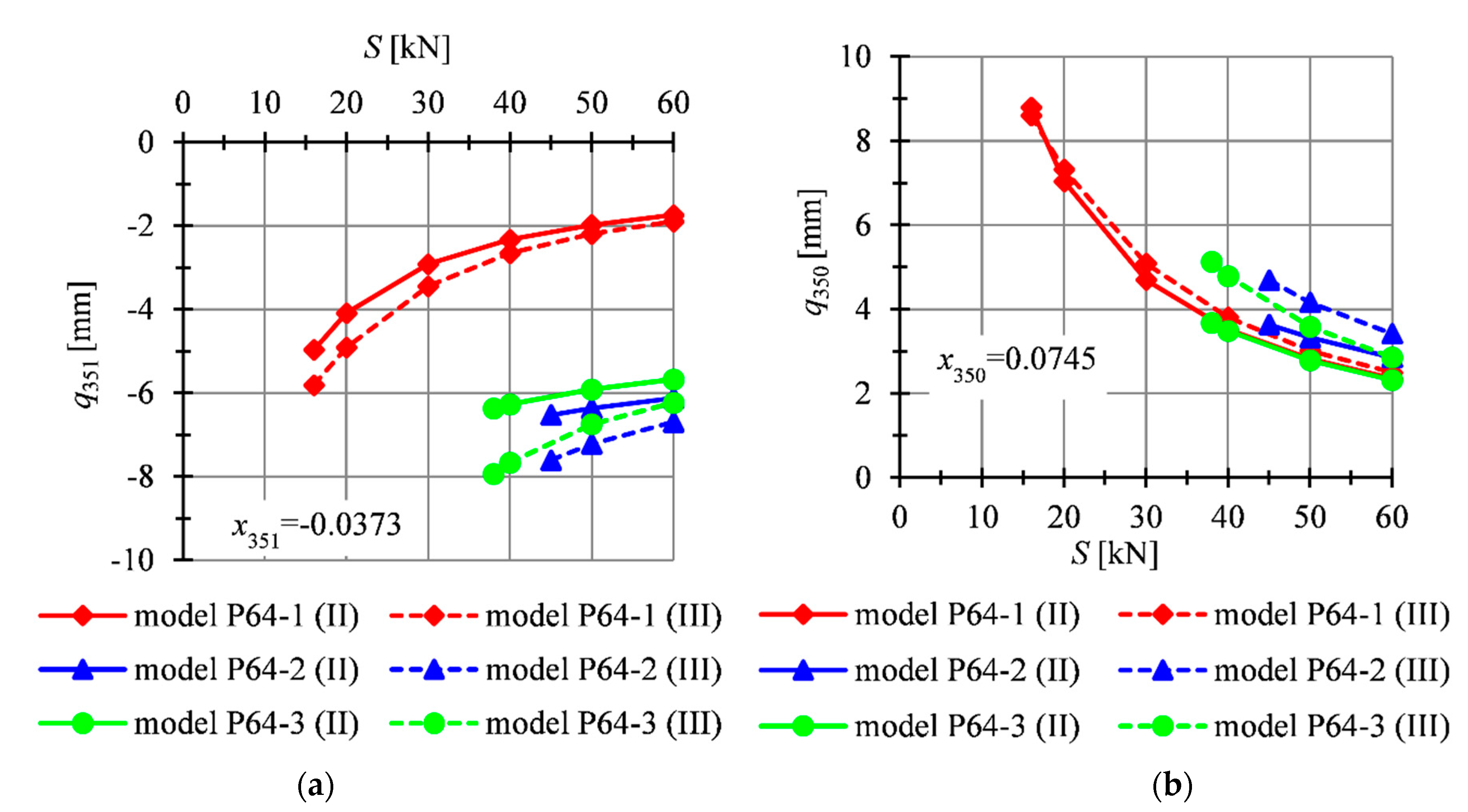
The last taken into account structure consists of sixty four modified Quartex modules (Figure 13a). Three models (models: P16-1–P16-3) with different way of support were considered in Part 1 [45]. All analyzed models (Figure 13b) are structures with tensegrity features of 1 class and the quantitative analysis is carried for these models. The minimum prestress level depends on the way of support. This level there is much higher than that obtained for the previous models and for three analysed models, i.e., P64-1, P64-2, and P64-3 equals, respectively, , and . The maximum prestress level is like in previous plates—.
The models were loaded by uniformly distributed load applied on the top surface of the structure. The influence of the initial prestress level on the non-zero displacements of 117th node (), the global stiffness parameter (), and the effort () are illustrated in Figure 14. Additionally, in Table 6 values of analyzed static parameters for the minimum and maximum prestress level are shown. Due to the quite high value of the minimum prestress level, the effect of non-linearity is not very significant. For example, in the case of the model P64-3, the relative error between the second (II) and third (III) order theory is equal to for and for for and, respectively, and for (Figure 14a,b). Additionally, it can be observed that for the models P64-2 and P64-3, the direction of supports is not as significant as in the case of analogically supported plates built with four modules (models P4-2 and P4-3).
The insignificant effect of non-linearity is also noticeable in the case of the global stiffness parameter (Figure 14c) and the effort (Figure 14d). The dependences on the initial prestress level S are almost linear, especially for the models P64-2–P64-3. Like in the previous plates, the effort of cables is higher than that of struts. For example, for the model P64-1, the effort of cables is 53.2% higher than of struts for and 59.7%. for .
5. Summary and Conclusions
The quantitative evaluation of truss structures presented in this paper was used for the assessment of the behaviour of tensegrity plate-like structures. The complete analysis of tensegrity structures is a two-stage process. The quantitative analysis carried out in this paper is the second stage and completes the qualitative analysis [45], which is the first stage. Defined in [45], the unique properties and the proposed classification of tensegrity structures (tensegrities were divided into four classes) are important due to the different behaviours of the structure under external actions. In this paper, it is proved that the stiffness of ideal and “pure” tensegrity structures and structures with tensegrity features of class 1 (structures in which mechanisms are identified) depends not only on the geometry and material properties, but also on the prestress level and external loads. However, it should be emphasized that the influence of self-equilibrium force system on the stabilization of the structure can be demonstrated only at the load that causes the displacements consistent with the infinitesimal mechanism. In other cases, the displacements are insensitive to changes of the prestress level. The existence of a state of self-stress in structures with tensegrity features of class 2 (structures in which mechanisms are not identified) allows for prestressing them, but they are insensitive to changes in the force level.
In this paper, a static parametric analysis of plates built with modified Quartex modules was carried out. Starting from a single-module structure, more complex cases were sequentially analyzed. The influence of the initial prestress level on the displacements, the effort and the stiffness of the structure was studied. For the determination of the structural stiffness, the global stiffness parameter () was proposed. This parameter determines the impact of self-stress state on the total rigidity of the structure at a given load. The calculation procedure, including the analysis of geometrically non-linear rod systems, was written in the Mathematica environment. The program makes it possible to freely define the geometry of the structure, material parameters, and loads, and then identify the self-stress state and track the behaviour of selected static and geometric parameters in the function of this state.
Before proceeding with the quantitative analysis of the tensegrity structure, a qualitative assessment is required. It leads to the classification of tensegrity structures. Stiffness control is possible only in structures characterized by the presence of an infinitesimal mechanism, which is the case of ideal or “pure” tensegrities and structures with tensegrity features of class 1. The stiffness of these structures depends not only on the geometry and material properties, but also on the prestress level (which stabilizes the infinitesimal mechanisms that occur) and the level of external load. External load induces additional stress in the system, and the impact of the load is most significant for the low values of the initial prestress forces. As the level of prestress increases, the effect of the external load decreases. Moreover, the initial prestress forces have a greater influence on the total stiffness of the structure with smaller external loads. Similarly, like for stiffness of tensegrity structures, in the case of effort, the influence of self-stress state decreases with increasing loads. The effort of cables is higher than that of struts and the difference between them increases with the increment of the prestress level.
The crucial aspect of the quantitative analyses is the determination of a prestress range, which is an individual feature of a tensegrity structure. The value of the minimum prestress level depends on the proper distribution of normal forces in the structure’s elements, i.e., tensile forces must be present in cables and compressive forces must be present in struts. In some cases, the external load causes a different distribution of normal forces, which can be corrected only by introducing an appropriate level of the initial prestress level. In turn, the value of the maximum prestress level depends on the load-bearing capacity of the most stressed elements.
The conducted analyses show that the effect of non-linearity is more significant for the low values of the initial prestress forces. The differences between values of the displacements obtained using the second and third order theory are significant when the prestress level is low. As the values of prestressing forces increase, the differences between the calculations performed according to the second and third order theory are becoming smaller. The differences between theories are also more significant for higher external load. The greatest impact of non-linearity occurs in the case of structures with a small value of the minimum prestress level (single-module structure and models: P4-1, P4-2, P4-3, P4-5, PS-1, P16-1). With increasing values of the minimum prestress level (models: P4-4, P64-1, P64-2, P64-3), the effect of non-linearity becomes smaller. Additionally, in the case of four-module plates, the direction of supports influences the displacements, whereas for strips and sixty-four-module plates does not.
For structure with tensegrity features of class 2 (without mechanisms), the global stiffness parameter is equal to 1 () and the effect of non-linearity is insignificant. The second order theory is sufficient for the purpose of analysis for such structures (the results obtained from the second and the third order theory are convergent).
The description presented in this paper is sufficient for quantitative analysis of planar and spatial lattice structures, including tensegrity structures, in the geometrically non-linear and physically linear setting. The proposed tensegrity plate-like structures can be used in the design process of standard tensegrity building structures, i.e., plates and non-standard applications.
Author Contributions
Introduction was prepared by J.T. Mathematical descriptions were written by P.O. Results were obtained by J.T. The analysis of the results was written by P.O. and J.T. Conclusions were written by P.O. All authors have read and agreed to the published version of the manuscript.
Funding
Project financed under the programme of the Minister of Science and Higher Education under the name “Regional Initiative of Excellence” in the years 2019–2022, project number 025/RID/2018/19, amount of financing 12 000 000 PLN.
Institutional Review Board Statement
Not applicable.
Informed Consent Statement
Not applicable.
Data Availability Statement
The data presented in this study is available in this article and [45].
Conflicts of Interest
The authors declare no conflict of interest.
References
- Zhang, L.-Y.; Zhu, S.-X.; Chen, X.-F.; Xu, G.-K. Analytical Form-Finding for Highly Symmetric and Super-Stable Configurations of Rhombic Truncated Regular Polyhedral Tensegrities. J. Appl. Mech. 2019, 86. [Google Scholar] [CrossRef]
- Schek, H.-J. The force density method for form finding and computation of general networks. Comput. Methods Appl. Mech. Eng. 1974, 3, 115–134. [Google Scholar] [CrossRef]
- Xu, X.; Wang, Y.; Luo, Y. Finding member connectivities and nodal positions of tensegrity structures based on force density method and mixed integer non-linear programming. Eng. Struct. 2018, 166, 240–250. [Google Scholar] [CrossRef]
- Barnes, M.R. Form Finding and Analysis of Tension Structures by Dynamic Relaxation. Int. J. Space Struct. 1999, 14, 89–104. [Google Scholar] [CrossRef]
- Domer, B.; Fest, E.; Lalit, V.; Smith, I.F.C. Combining Dynamic Relaxation Method with Artificial Neural Networks to Enhance Simulation of Tensegrity Structures. J. Struct. Eng. 2003, 129, 672–681. [Google Scholar] [CrossRef] [Green Version]
- Estrada, G.G.; Bungartz, H.-J.; Mohrdieck, C. Numerical form-finding of tensegrity structures. Int. J. Solids Struct. 2006, 43, 6855–6868. [Google Scholar] [CrossRef] [Green Version]
- Pagitz, M.; Mirats Tur, J.M. Finite element based form-finding algorithm for tensegrity structures. Int. J. Solids Struct. 2009, 46, 3235–3240. [Google Scholar] [CrossRef]
- Tran, H.C.; Lee, J. Advanced form-finding of tensegrity structures. Comput. Struct. 2010, 88, 237–246. [Google Scholar] [CrossRef]
- Koohestani, K.; Guest, S.D. A new approach to the analytical and numerical form-finding of tensegrity structures. Int. J. Solids Struct. 2013, 50, 2995–3007. [Google Scholar] [CrossRef] [Green Version]
- Lee, S.; Lee, J.; Kang, J. A Genetic Algorithm Based Form-finding of Tensegrity Structures with Multiple Self-stress States. J. Asian Archit. Build. Eng. 2017, 16, 155–162. [Google Scholar] [CrossRef] [Green Version]
- Djouadi, S.; Motro, R.; Pons, J.C.; Crosnier, B. Active Control of Tensegrity Systems. J. Aerosp. Eng. 1998, 11, 37–44. [Google Scholar] [CrossRef]
- Fest, E.; Shea, K.; Smith Ian, F.C. Active Tensegrity Structure. J. Struct. Eng. 2004, 130, 1454–1465. [Google Scholar] [CrossRef] [Green Version]
- Domer, B.; Smith, I.F.C. An Active Structure that Learns. J. Comput. Civ. Eng. 2005, 19, 16–24. [Google Scholar] [CrossRef] [Green Version]
- Adam, B.; Smith, I.F.C. Active tensegrity: A control framework for an adaptive civil-engineering structure. Comput. Struct. 2008, 86, 2215–2223. [Google Scholar] [CrossRef] [Green Version]
- Raja, M.G.; Narayanan, S. Active control of tensegrity structures under random excitation. Smart Mater. Struct. 2007, 16, 809–817. [Google Scholar] [CrossRef]
- Sabouni-Zawadzka, A. Active Control of Smart Tensegrity Structures. Arch. Civ. Mech. Eng. 2014, 60, 517–534. [Google Scholar] [CrossRef]
- Amouri, S.; Averseng, J.; Dubé, J.-F. Active control design of modular tensegrity structures. In Proceedings of the International Association for Shell and Spatial Structures (IASS) Symposium 2013, Wroclaw, Poland, 23–27 September 2013. [Google Scholar]
- Oliveto, N.D.; Sivaselvan, M.V. Dynamic analysis of tensegrity structures using a complementarity framework. Comput. Struct. 2011, 89, 2471–2483. [Google Scholar] [CrossRef]
- Fraternali, F.; Senatore, L.; Daraio, C. Solitary waves on tensegrity lattices. J. Mech. Phys. Solids 2012, 60, 1137–1144. [Google Scholar] [CrossRef]
- Faroughi, S.; Lee, J. Analysis of tensegrity structures subject to dynamic loading using a Newmark approach. J. Build. Eng. 2015, 2, 1–8. [Google Scholar] [CrossRef]
- Ashwear, N.; Tamadapu, G.; Eriksson, A. Optimization of modular tensegrity structures for high stiffness and frequency separation requirements. Int. J. Solids Struct. 2016, 80, 297–309. [Google Scholar] [CrossRef]
- Kan, Z.; Peng, H.; Chen, B.; Zhong, W. Non-linear dynamic and deployment analysis of clustered tensegrity structures using a positional formulation FEM. Compos. Struct. 2018, 187, 241–258. [Google Scholar] [CrossRef]
- Tibert, G.; Pellegrino, S. Deployable Tensegrity Reflectors for Small Satellites. J. Spacecr. Rockets. 2002, 39, 701–709. [Google Scholar] [CrossRef] [Green Version]
- Veuve, N.; Safaei, S.; Smith, I. Deployment of a Tensegrity Footbridge. J. Struct. Eng. 2015, 141, 04015021. [Google Scholar] [CrossRef] [Green Version]
- Gilewski, W.; Kłosowska, J.; Obara, P. Applications of Tensegrity Structures in Civil Engineering. Procedia Eng. 2015, 111, 242–248. [Google Scholar] [CrossRef] [Green Version]
- Wang, Z.; Li, K.; He, Q.; Cai, S. A Light-Powered Ultralight Tensegrity Robot with High Deformability and Load Capacity. Adv. Mater. 2019, 31, 1806849. [Google Scholar] [CrossRef]
- Park, S.; Park, E.; Yim, M.; Kim, J.; Seo, T.W. Optimization-Based Nonimpact Rolling Locomotion of a Variable Geometry Truss. IEEE Robot. Autom. Lett. 2019, 4, 747–752. [Google Scholar] [CrossRef]
- Zhang, Q.; Zhang, D.; Dobah, Y.; Scarpa, F.; Fraternali, F.; Skelton, R.E. Tensegrity cell mechanical metamaterial with metal rubber. Appl. Phys. Lett. 2018, 113, 031906. [Google Scholar] [CrossRef] [Green Version]
- Fabbrocino, F.; Carpentieri, G. Three-dimensional modeling of the wave dynamics of tensegrity lattices. Compos. Struct. 2017, 173, 9–16. [Google Scholar] [CrossRef]
- Fraddosio, A.; Marzano, S.; Pavone, G.; Piccioni, M.D. Morphology and self-stress design of V-Expander tensegrity cells. Compos. Part B Eng. 2017, 115, 102–116. [Google Scholar] [CrossRef]
- Sabouni-Zawadzka, A.; Gilewski, W. Soft and Stiff Simplex Tensegrity Lattices as Extreme Smart Metamaterials. Materials 2019, 12, 187. [Google Scholar] [CrossRef] [Green Version]
- Gilewski, W.; Sabouni-Zawadzka, A. On possible applications of smart structures controlled by self-stress. Arch. Civ. Mech. Eng. 2014, 15, 469–478. [Google Scholar] [CrossRef]
- Hanaor, A.; Liao, M.-K. Double-Layer Tensegrity Grids: Static Load Response. Part I: Analytical Study. J. Struct. Eng. 1991, 117, 1660–1674. [Google Scholar] [CrossRef]
- Hanaor, A. Double-Layer Tensegrity Grids: Static Load Response. Part II: Experimental Study. J. Struct. Eng. 1991, 117, 1675–1684. [Google Scholar] [CrossRef]
- Murakami, H. Static and dynamic analyses of tensegrity structures. Part 1. Non-linear equations of motion. Int. J. Solids Struct. 2001, 38, 3599–3613. [Google Scholar] [CrossRef]
- Murakami, H. Static and dynamic analyses of tensegrity structures. Part II. Quasi-static analysis. Int. J. Solids Struct. 2001, 38, 3615–3629. [Google Scholar] [CrossRef]
- Fu, F. Non-linear static analysis and design of Tensegrity domes. Steel Compos. Struct. 2006, 6, 417–433. [Google Scholar] [CrossRef] [Green Version]
- Angellier, N.; Dubé, J.F.; Quirant, J.; Crosnier, B. Behavior of a Double-Layer Tensegrity Grid under Static Loading: Identification of Self-Stress Level. J. Struct. Eng. 2013, 139, 1075–1081. [Google Scholar] [CrossRef] [Green Version]
- Gilewski, W.; Obara, P.; Kłosowska, J. Self-stress control of real civil engineering tensegrity structures. AIP Conf. Proc. 2018, 1922, 150004. [Google Scholar]
- Gilewski, W.; Kłosowska, J.; Obara, P. Parametric analysis of some tensegrity structures. MATEC Web Conf. 2019, 262, 10003. [Google Scholar] [CrossRef]
- Gilewski, W.; Kłosowska, J.; Obara, P. The influence of self-stress on the behavior of tensegrity-like real structure. MATEC Web Conf. 2017, 117, 00079. [Google Scholar] [CrossRef] [Green Version]
- Obara, P. Analysis of orthotropic tensegrity plate strips using a continuum two-dimensional model. MATEC Web Conf. 2019, 262, 10010. [Google Scholar] [CrossRef]
- Obara, P. Application of linear six-parameter shell theory to the analysis of orthotropic tensegrity plate-like structures. J. Theor. App. Mech. 2019, 57, 167–178. [Google Scholar] [CrossRef]
- Obara, P. Dynamic and Dynamic Stability of Tensegrity Structures; Wydawnictwo Politechniki Świętokrzyskiej: Kielce, Poland, 2019. (In Polish) [Google Scholar]
- Obara, P.; Tomasik, J. Parametric Analysis of Tensegrity Plate-Like Structures: Part 1—Qualitative Analysis. Appl. Sci. 2020, 10, 7042. [Google Scholar] [CrossRef]
- Argyris, J.; Scharpf, D.W. Large Deflection Analysis of Prestressed Networks. J. Struct. Div. 1972, 98, 633–654. [Google Scholar]
- Motro, R. Forms and Forces in Tensegrity Systems. In Proceedings of the Third International Conference on Space Structures, Amsterdam, The Netherlands, 11–14 September 1984; Nooshin, H., Ed.; Elsevier: London, UK, 1984; pp. 180–185. [Google Scholar]
- Kebiche, K.; Kazi-Aoual, M.N.; Motro, R. Geometrical non-linear analysis of tensegrity systems. Eng. Struct. 1999, 21, 864–876. [Google Scholar] [CrossRef]
- Tran, H.C.; Lee, J. Geometric and material non-linear analysis of tensegrity structures. Acta Mech. Sin. 2011, 27, 938–949. [Google Scholar] [CrossRef]
- Faroughi, S.; Lee, J. Geometrical Non-linear Analysis of Tensegrity Based on a Co-Rotational Method. Adv. Struct. Eng. 2014, 17, 41–51. [Google Scholar] [CrossRef]
- Szmelter, J. Computer Methods in Mechanics; Państwowe Wydawnictwo Naukowe: Warsaw, Poland, 1980. [Google Scholar]
- Crisfield, M.A. Non-Linear Finite Element Analysis of Solids and Structures, Essentials; Wiley: Hoboken, NJ, USA, 1991; ISBN 978-0-471-92956-7. [Google Scholar]
- Bathe, K.-J. Finite Element Procedures in Engineering Analysis; Prentice-Hall: New York, NY, USA, 1982. [Google Scholar]
- Borst, R.; Crisfield, M.; Remmers, J.; Verhoosel, C. Non-Linear Finite Element Analysis of Solids and Structures: Second Edition; Wiley: Chichester, UK, 2012. [Google Scholar]
- Rakowski, G.; Kacprzyk, Z. Finite Element Method in Structural Mechanics; Oficyna Wydawnicza Politechniki Warszawskiej: Warsaw, Poland, 2016. [Google Scholar]
Figure 1.
Space finite tensegrity element.
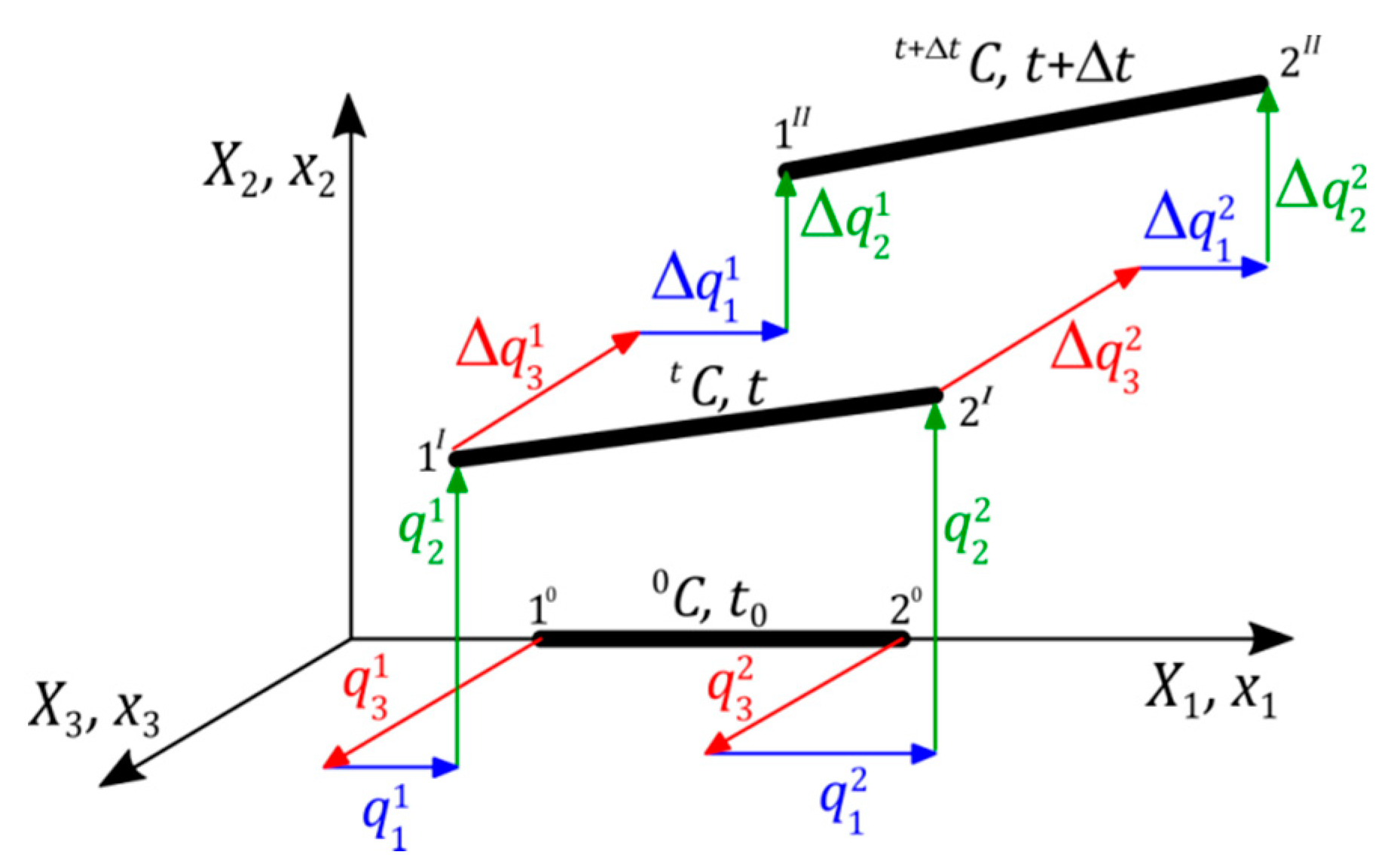
Figure 2.
The single modified Quartex module: (a) geometry, (b) normalised self-stress state .
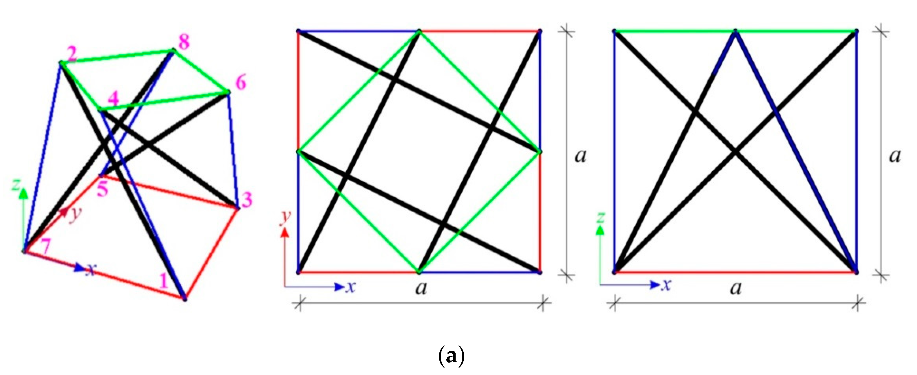
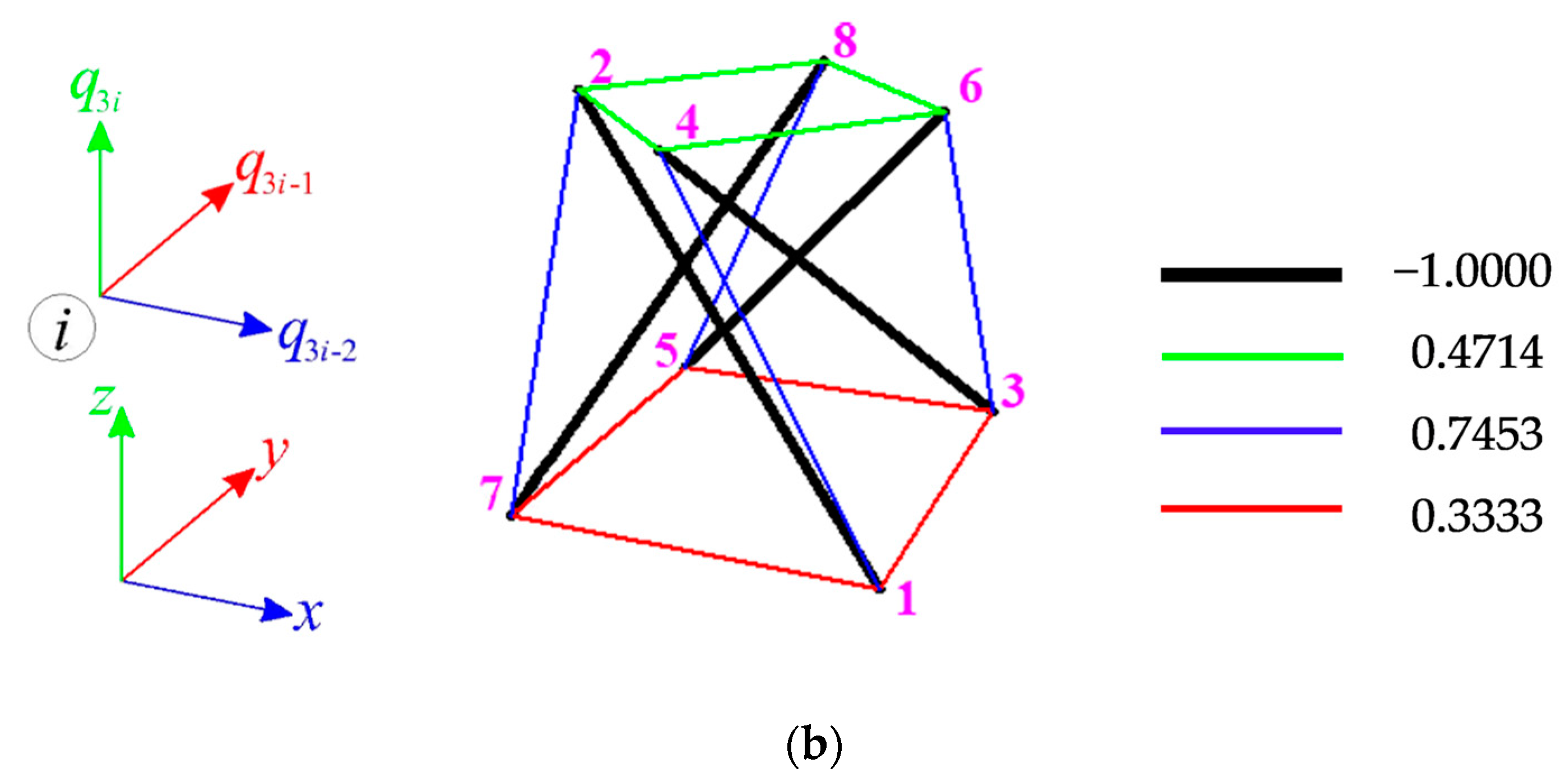
Figure 3.
Impact of the initial prestress level S on the: (a) displacement , (b) displacement , (c) global stiffness parameter , and (d) effort of structure .
Figure 3.
Impact of the initial prestress level S on the: (a) displacement , (b) displacement , (c) global stiffness parameter , and (d) effort of structure .

Figure 4.
Four-module tensegrity plate-like structure: (a) geometry, (b) models of structures with tensegrity features of class 1, and (c) model of structure with tensegrity features of class 2.
Figure 4.
Four-module tensegrity plate-like structure: (a) geometry, (b) models of structures with tensegrity features of class 1, and (c) model of structure with tensegrity features of class 2.
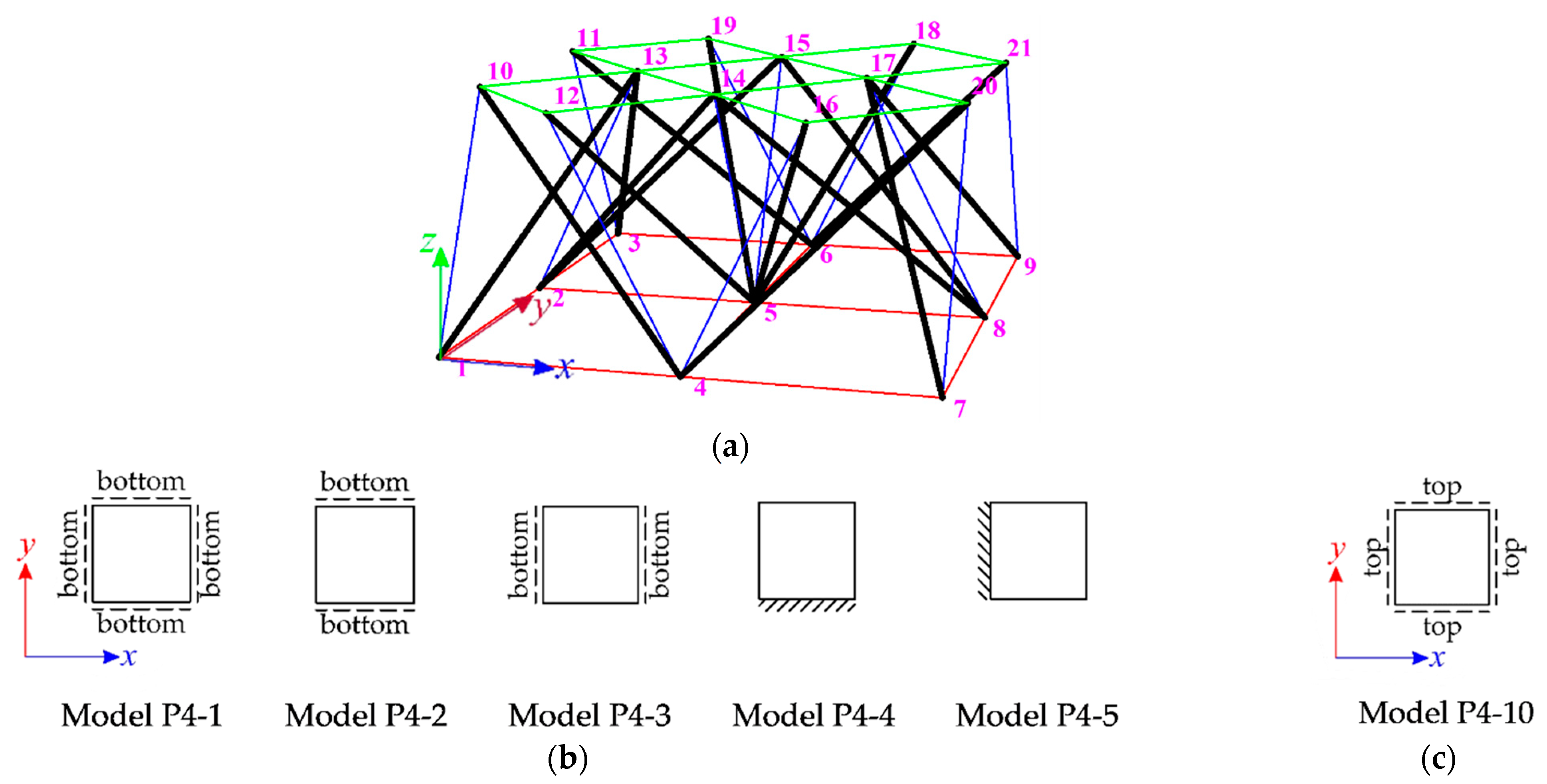
Figure 5.
Impact of the initial prestress level S on the displacements: (a) , (b) , (c) .
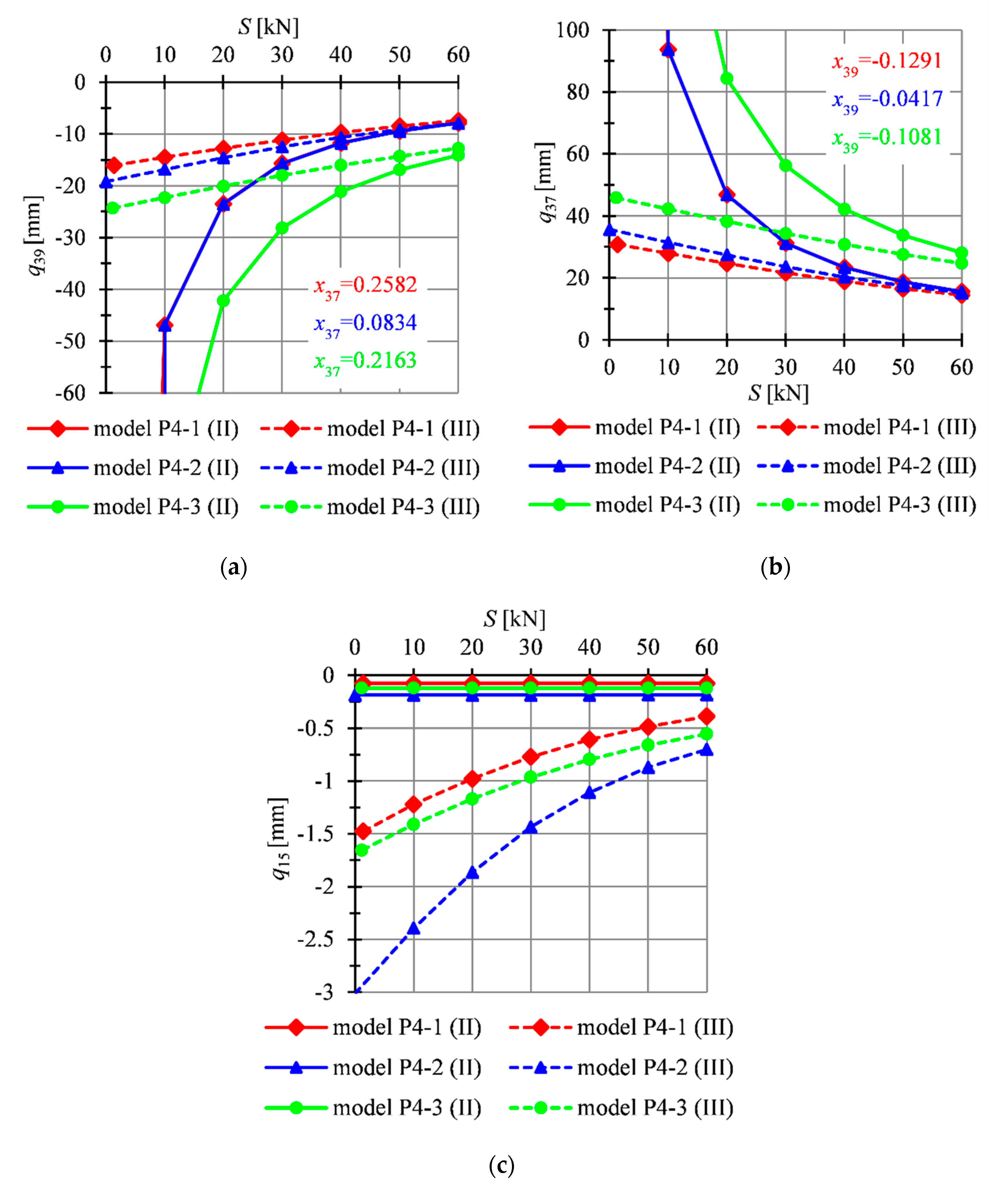
Figure 6.
Impact of the initial prestress level S on the: (a) global stiffness parameter , (b) effort of structure .
Figure 6.
Impact of the initial prestress level S on the: (a) global stiffness parameter , (b) effort of structure .
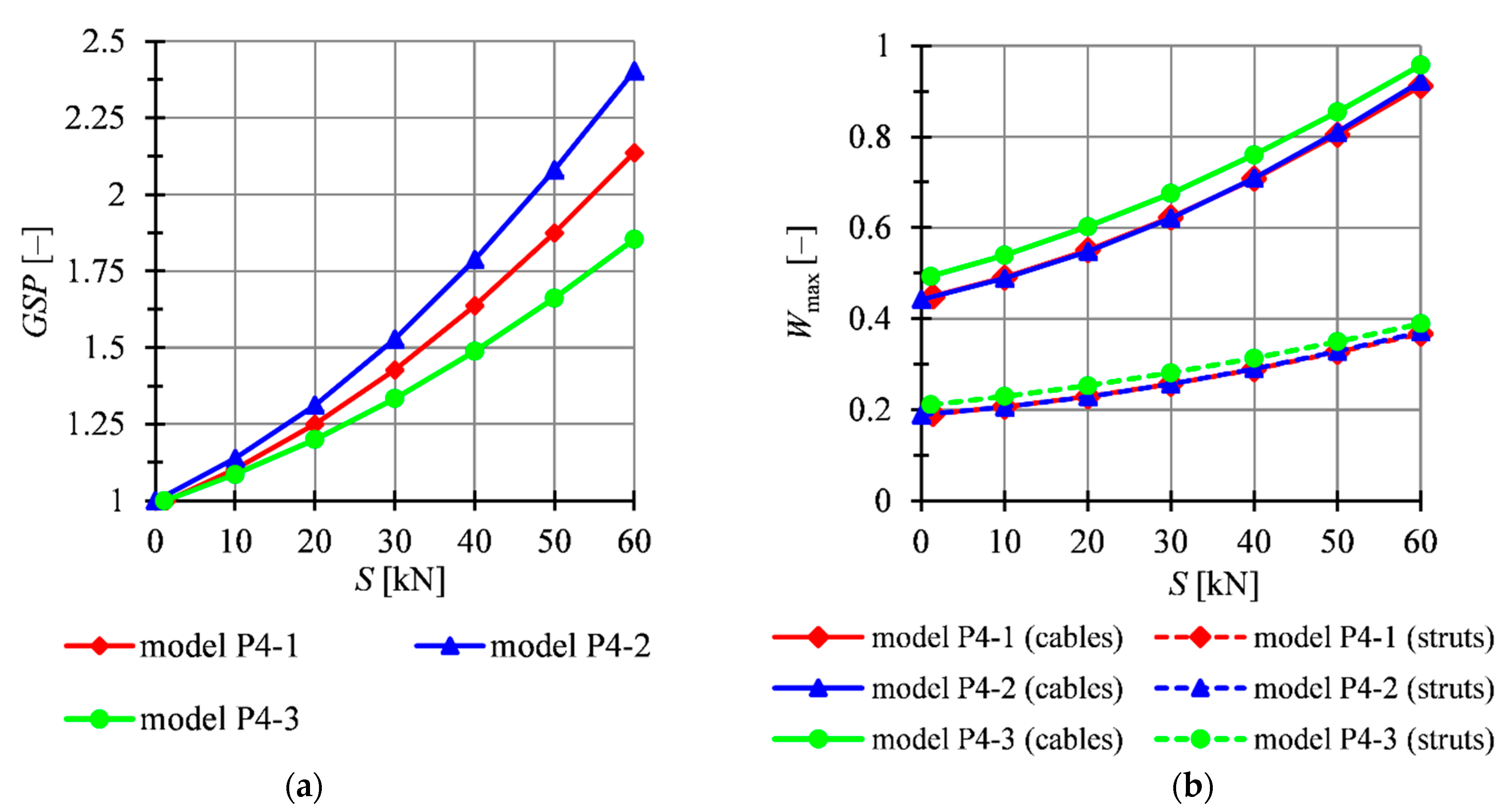
Figure 7.
Impact of the initial prestress level S on the: (a) bottom nodes’ displacements, (b) top nodes’ displacements, (c) global stiffness parameter , (d) effort of structure .
Figure 7.
Impact of the initial prestress level S on the: (a) bottom nodes’ displacements, (b) top nodes’ displacements, (c) global stiffness parameter , (d) effort of structure .
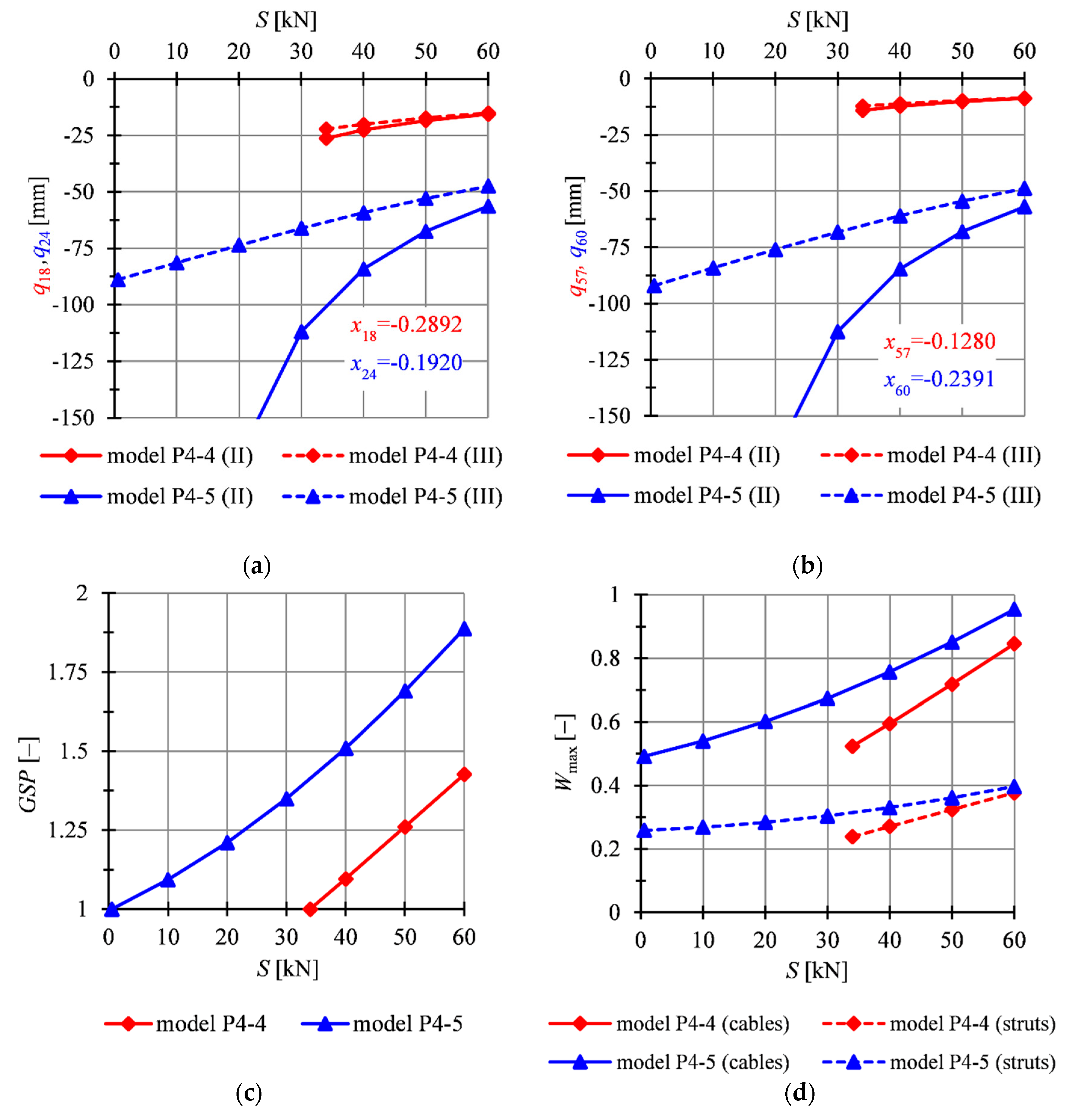
Figure 8.
Impact of the initial prestress level S on the displacements: (a) , (b) , (c) .
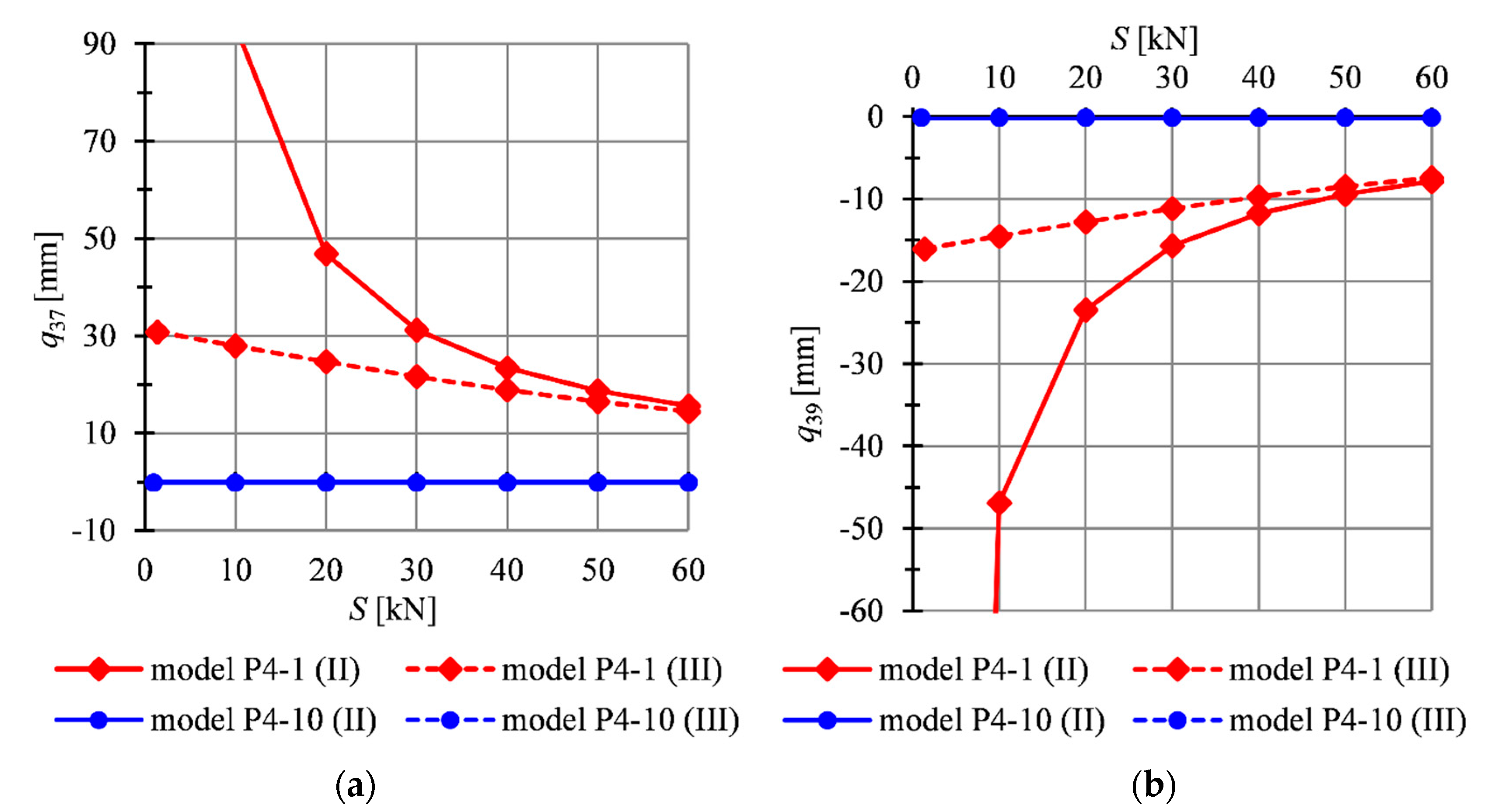

Figure 9.
Impact of the initial prestress level S on the: (a) global stiffness parameter , (b) effort of structure .
Figure 9.
Impact of the initial prestress level S on the: (a) global stiffness parameter , (b) effort of structure .
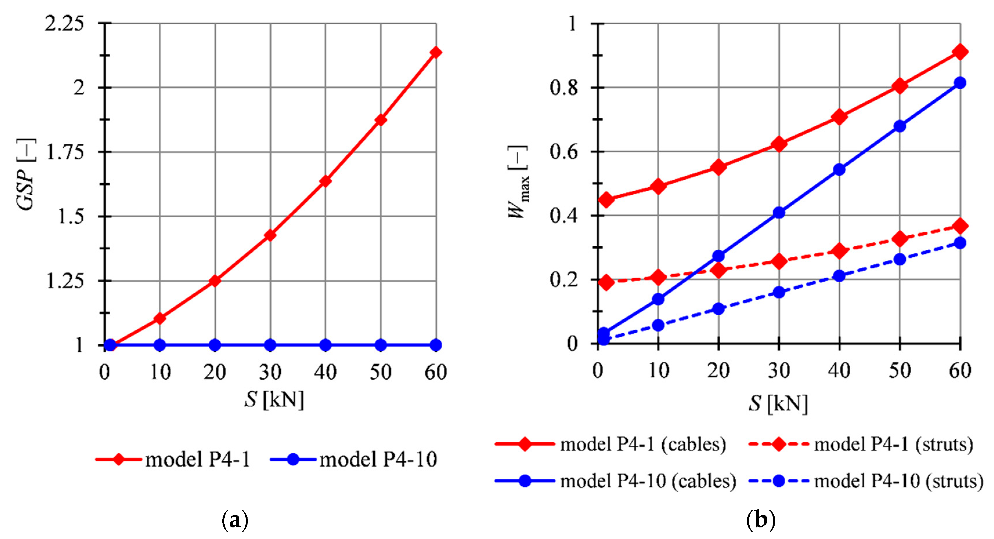
Figure 10.
Sixteen-module tensegrity plate-like structure: (a) top view, (b) model of structures with tensegrity features of class 1, (c) model of structures with tensegrity features of class 2.
Figure 10.
Sixteen-module tensegrity plate-like structure: (a) top view, (b) model of structures with tensegrity features of class 1, (c) model of structures with tensegrity features of class 2.
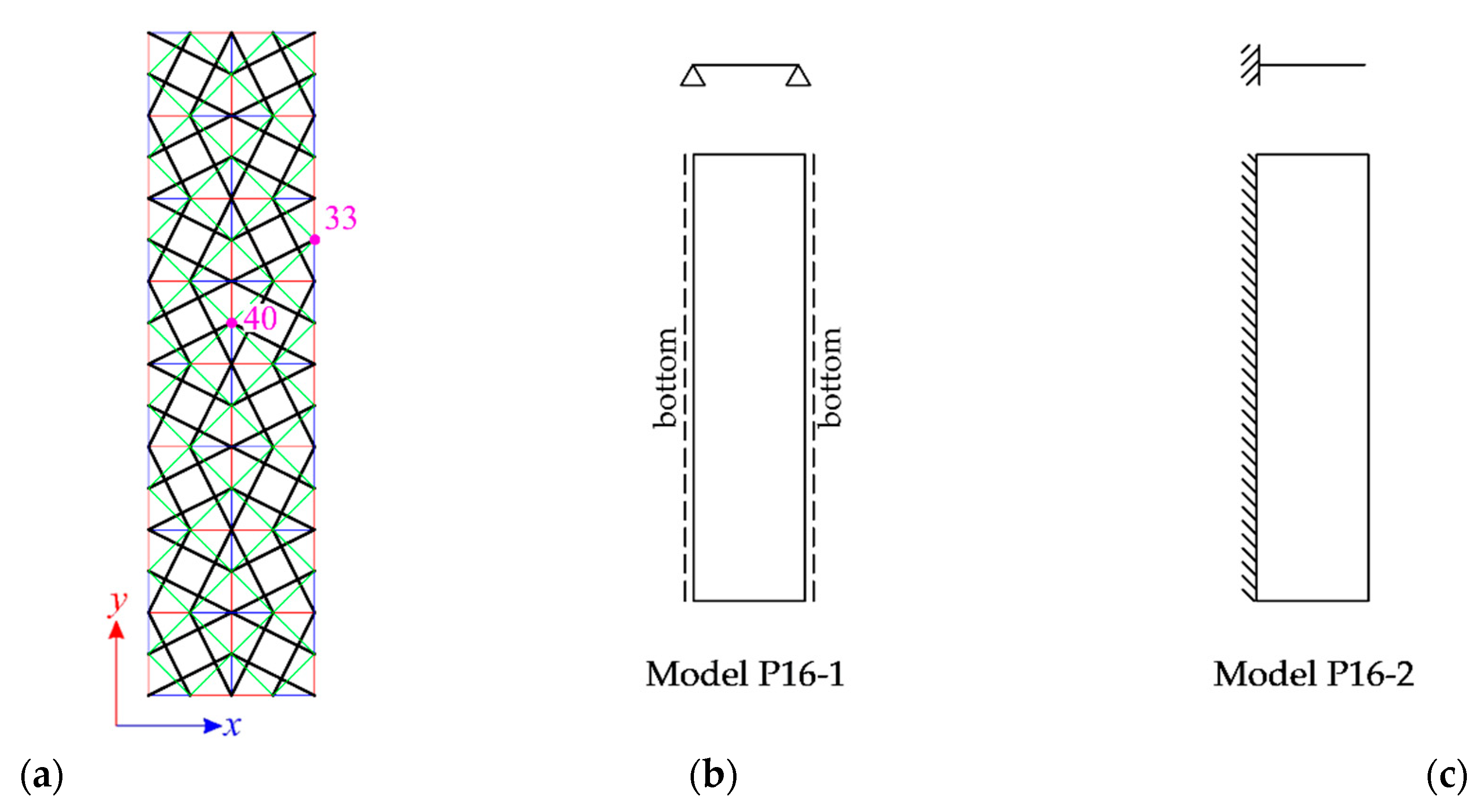
Figure 11.
Models of the tensegrity plate strips.
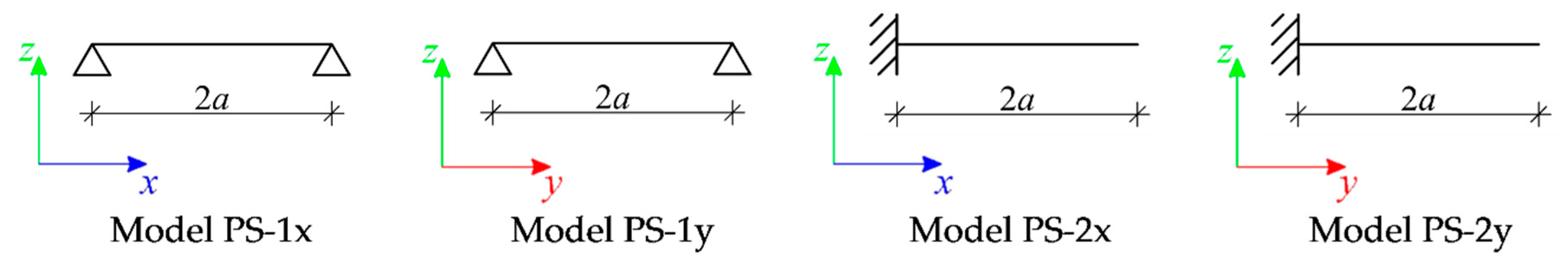
Figure 12.
Impact of the initial prestress level S on the: (a) global stiffness parameter GSP, (b) effort of structure .
Figure 12.
Impact of the initial prestress level S on the: (a) global stiffness parameter GSP, (b) effort of structure .

Figure 13.
Sixty-four-module tensegrity plate-like structure: (a) geometry, (b) models of structures with tensegrity features of class 1.
Figure 13.
Sixty-four-module tensegrity plate-like structure: (a) geometry, (b) models of structures with tensegrity features of class 1.
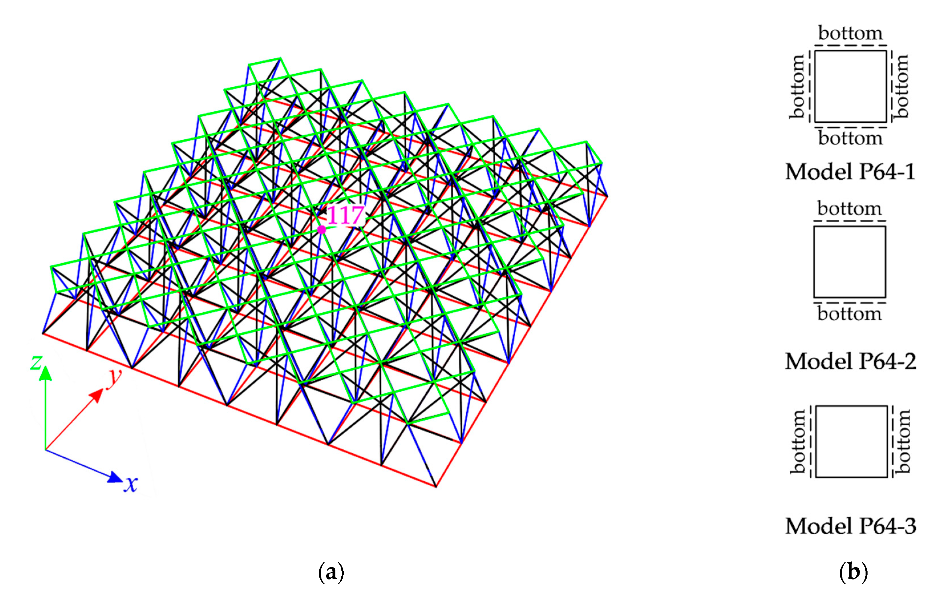
Figure 14.
Impact of the initial prestress level S on the: (a) displacement , (b) displacement , (c) global stiffness parameter GSP, (d) effort of structure .
Figure 14.
Impact of the initial prestress level S on the: (a) displacement , (b) displacement , (c) global stiffness parameter GSP, (d) effort of structure .


Table 1.
Load-bearing characteristics of the single modified Quartex module.
| S [kN] | Type of Element | |||||||||
|---|---|---|---|---|---|---|---|---|---|---|
| 0.01 | cables | 26.5 | 0.241 | 1.0 | 35.7 | 0.324 | 1.0 | 44.1 | 0.400 | 1.0 |
| struts | −35.6 | 0.184 | −47.8 | 0.246 | 59.1 | 0.305 | ||||
| 110 | cables | 87.3 | 0.792 | 3.7 | 91.1 | 0.826 | 2.9 | 95.3 | 0.865 | 2.5 |
| struts | −117.2 | 0.604 | −122.2 | 0.630 | −128.0 | 0.660 | ||||
Table 2.
Load-bearing characteristics of the models P4-1–P4-3.
| S [kN] | Type of Element | Model P4-1 () | Model P4-2 | Model P4-3 | ||||||
|---|---|---|---|---|---|---|---|---|---|---|
| Smin | cables | 49.54 | 0.450 | 1.0 | 48.8 | 0.443 | 1.0 | 54.4 | 0.493 | 1.0 |
| struts | −37.0 | 0.191 | −36.6 | 0.189 | −41.0 | 0.211 | ||||
| 60 | cables | 100.5 | 0.912 | 2.1 | 101.5 | 0.921 | 2.4 | 105.6 | 0.958 | 1.9 |
| struts | −71.2 | 0.367 | −71.93 | 0.371 | −75.4 | 0.389 | ||||
Table 3.
Load-bearing characteristics of the models P4-4 and P4-5.
| S [kN] | Type of Element | Model P4-4 | Model P4-5 | ||||
|---|---|---|---|---|---|---|---|
| Smin | cables | 57.7 | 0.524 | 1.0 | 54.1 | 0.491 | 1.0 |
| struts | −46.3 | 0.239 | −50.1 | 0.258 | |||
| 60 | cables | 93.2 | 0.846 | 1.4 | 105.2 | 0.954 | 1.9 |
| struts | −73.1 | 0.376 | −77.0 | 0.397 | |||
Table 4.
Comparison of the displacements for four-module plate strips and the sixteen-module plates.
Table 4.
Comparison of the displacements for four-module plate strips and the sixteen-module plates.
| Simply Supported | Cantilever | ||||||||
|---|---|---|---|---|---|---|---|---|---|
| Second Order Theory | Third Order Theory | Second Order Theory | |||||||
| S | Plate Strip PS-1x | Plate Model P16-1 | Relative Error | Plate Strip PS-1x | Plate Model P16-1 | Relative Error | Plate Strip PS-2x | Plate Model P16-2 | Relative Error |
| [mm] | [mm] | [%] | [mm] | [mm] | [%] | [mm] | [mm] | [%] | |
| 3 | −156.339 | −156.342 | 0.00 | −17.056 | −17.605 | −3.11 | − | − | − |
| 10 | −46.965 | −46.967 | −0.01 | −15.672 | −16.131 | −2.85 | − | − | − |
| 21 | −23.527 | −23.530 | −0.01 | −13.751 | −14.091 | −2.41 | −0.737 | −0.793 | −7.08 |
| 30 | −15.715 | −15.717 | −0.02 | −11.954 | −12.193 | −1.95 | −0.736 | −0.793 | −7.08 |
| 40 | −11.808 | −11.811 | −0.02 | −10.345 | −10.505 | −1.52 | −0.736 | −0.792 | −7.07 |
| 50 | −9.465 | −9.467 | −0.03 | −8.962 | −9.066 | −1.15 | −0.736 | −0.792 | −7.07 |
| 60 | −7.902 | −7.905 | −0.03 | −7.810 | −7.878 | −0.86 | −0.735 | −0.791 | −7.08 |
Table 5.
Load-bearing characteristics of the models PS-1.
| S [kN] | Type of Element | Model PS-1x () | Model PS-1y () | ||||
|---|---|---|---|---|---|---|---|
| Smin | cables | 54.1 | 0.491 | 1.0 | 52.7 | 0.478 | 1.0 |
| struts | −40.2 | 0.207 | −39.2 | 0.202 | |||
| 60 | cables | 103.3 | 0.937 | 2.2 | 102.6 | 0.931 | 2.2 |
| struts | −73.0 | 0.377 | −72.5 | 0.374 | |||
Table 6.
Load-bearing characteristics of the models P64-1–P64-3.
| S [kN] | Type of Element | Model P64-1 () | Model P64-2 () | Model P64-3 () | ||||||
|---|---|---|---|---|---|---|---|---|---|---|
| Smin | cables | 28.9 | 0.262 | 1.0 | 72.5 | 0.658 | 1.0 | 64.8 | 0.588 | 1.0 |
| struts | −23.7 | 0.123 | −63.0 | 0.324 | −58.4 | 0.301 | ||||
| 60 | cables | 91.1 | 0.827 | 3.3 | 94.4 | 0.857 | 1.2 | 97.0 | 0.880 | 1.3 |
| struts | −64.6 | 0.333 | −77.9 | 0.402 | 79.9 | 0.412 | ||||
Publisher’s Note: MDPI stays neutral with regard to jurisdictional claims in published maps and institutional affiliations. |
© 2021 by the authors. Licensee MDPI, Basel, Switzerland. This article is an open access article distributed under the terms and conditions of the Creative Commons Attribution (CC BY) license (http://creativecommons.org/licenses/by/4.0/).
Share and Cite
MDPI and ACS Style
Obara, P.; Tomasik, J. Parametric Analysis of Tensegrity Plate-Like Structures: Part 2—Quantitative Analysis. Appl. Sci. 2021, 11, 602. https://doi.org/10.3390/app11020602
AMA Style
Obara P, Tomasik J. Parametric Analysis of Tensegrity Plate-Like Structures: Part 2—Quantitative Analysis. Applied Sciences. 2021; 11(2):602. https://doi.org/10.3390/app11020602
Chicago/Turabian StyleObara, Paulina, and Justyna Tomasik. 2021. "Parametric Analysis of Tensegrity Plate-Like Structures: Part 2—Quantitative Analysis" Applied Sciences 11, no. 2: 602. https://doi.org/10.3390/app11020602
Note that from the first issue of 2016, this journal uses article numbers instead of page numbers. See further details here.