Active Earth Pressure of Limited C-φ Soil Based on Improved Soil Arching Effect

Featured Application

This study extends the previous active earth pressure studies to include c-φ soil of limited width in a dense underground environment by considering the soil-wall interaction and the ground surface overload.

Abstract

For c-φ soil formation (cohesive soil) of limited width with ground surface overload behind a deep retaining structure, a modified active earth pressure calculation model is established in this study. And three key issues are addressed through improved soil arching effect. First, the soil-wall interaction mechanism is determined by considering the soil arching effect. The slip surface of a limited soil is proved to be a double-fold line passing through the retaining wall toe and intersecting the side wall of the existing underground structure until it reaches the ground surface along the existing side wall. Second, the limited width boundary is explicated. And third, the variation in the active earth pressure from parameters of limited c-φ soil is determined. The lateral active earth pressure coefficient is nonlinear distributed based on the improved soil arching effect of the symmetric catenary curve. Furthermore, the active earth pressure distribution, the tension crack at the top of the retaining wall and the resultant force and its action point were obtained. By comparing with the existing analytical methods, such as the Rankine method, it demonstrates that the model proposed in this study is much closer to the measured and numerical results. Ignoring the influence of soil cohesion and the limited width will exponentially reduce the overall stability of the retaining structure and increase the risk of accidents.

1. Introduction

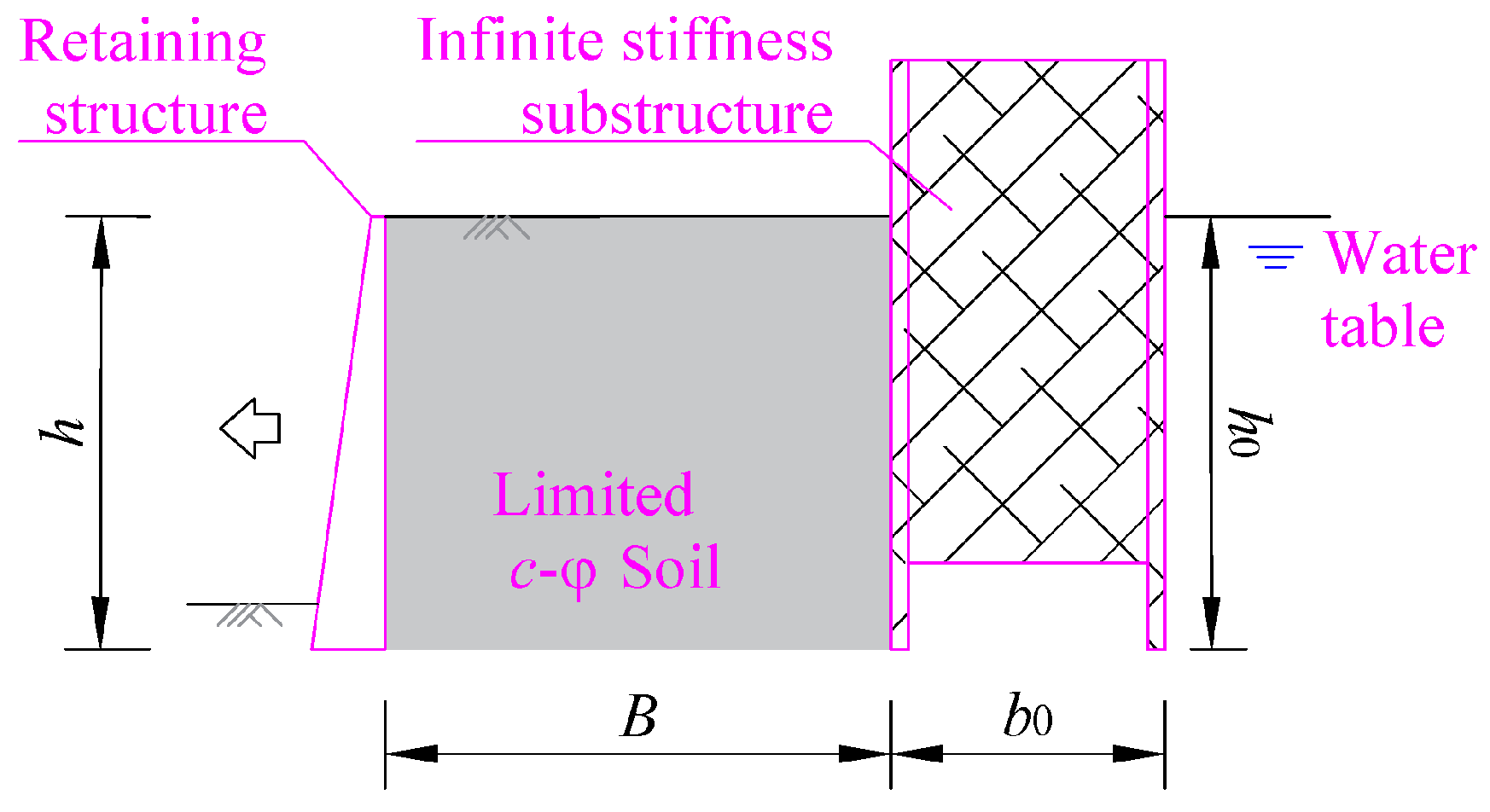
As the development of construction technology and density of the underground environment, the surrounding soil behind a deep retaining wall is often constrained by many underground structures. For example, a large number of underground projects, including but not limited to deep foundation pits, slope protection, and underground pipe corridors, occur near existing large-rigid underground structures, such as an existing deep basement or an operating subway station, as shown in Figure 1. The force and deformation of soil behind the deep retaining structure cannot pass through the side wall of an adjacent existing large rigid underground structure. Thus, a soil mass with a limited width is formed. The stress and strain of the limited soil are significantly different from those of a semi-infinite soil [1,2,3,4]. In this case, a reasonable soil of limited width between the newly constructed deep retaining wall and the existing underground structure must be scientifically considered. And the traditional Rankine method or Coulomb method is not suitable. It is still unclear whether the effect of the existing large-rigid underground structure on the clipped soil of limited width—and thus on the retaining structure—is positive or negative, especially when the soil condition is not simply dry sand.

Many studies investigated the active earth pressure distribution behind a deep retaining wall with limited c-φ soil (cohesive soil) [1,2,3,4,5,6,7,8,9,10,11,12,13,14,15,16,17] through multiple kinds of methods. Centrifuge model tests and field measurements [5,6,7,8,9,10] have been conducted to analyze the active earth pressure distribution of different limited soil widths, providing a great deal of valuable data for the future analysis. Numerical solutions [11,12,13,14] have also been implemented due to their comprehensiveness in considering multiple influencing factors if a suitable mechanical model and boundary conditions are considered carefully. Theoretical methods [15,16,17,18,19] have been introduced to ensure that the results of the field measurements, model tests, and numerical simulations are scientifically expressed and conveniently applied. Scholars [7,15,17,18,19] have incorporated the limited soil width into their calculations of the active earth pressure. The active earth pressure gradually increases with increasing of limited soil width. However, these methods do not consider the influence of soil cohesion [20,21,22,23,24,25,26] and ground surface overload [27,28,29], which are important factors in the design of a retaining structure. Further, these methods did not specify the explicit range of limited soil width.

A proper analytical method is needed for calculating the active earth pressure acting on the retaining wall. The limit equilibrium method of a horizontal soil strip [30,31,32,33,34,35] has been widely used because of its convenience and briefness in practical applications. And the methods for calculating the lateral coefficient of active earth pressure include moment equilibrium method [36,37] and the soil arching method [38,39,40]. The moment equilibrium method does not consider the force transmitted by the soil arching, which leads to the calculation results being inconsistent with the actual values. The soil arching effect is a common phenomenon caused by the transfer of internal stress, such as the earth pressure decreasing in the yield region and increasing in the adjacent region [41]. And it is more notable in the soil of limited width between two wall faces. Thus, the soil arching method is used and improved in the limit equilibrium method of a horizontal soil strip for calculating the active earth pressure of limited soil in this study.

Two main key problems about stress redistribution in the soil arching method include the stress direction deflection and the stress transfer path [39], and they are all reflected by the uneven deformation. The key problems are determined by the slip surface shape and the small principal stress trajectory [9,42]. Different types of slip surface shape have been proposed by theoretical assumptions and model tests, such as plane [43,44], cycloid [45], logarithmic spirals [46], and polylines [15,16]. Rankine plane slip surface [1,29,43,44] is widely used in the traditional soil arching method. However, the Rankine plane slip surface is only suitable for soil of semi-infinite width and for a smooth retaining wall. Moreover, the formulas of cycloid and logarithmic spirals are too complex to be used in practice. Many kinds of arching curves for simulating the small principal stress trajectory, such as arc [39], catenary [17], and parabola [47] have been proposed. There is still no evidence to suggest which kinds of slip surface shape and small principal stress trajectory are closer to the stress redistribution of the limited c-φ soil behind a retaining wall.

There are still no systematic studies to evaluate the active earth pressure for the limited c-φ soil between a deep retaining wall and an existing large-rigid underground structure when there is ground surface overload. The purpose of this study is to extend the previous studies to include the limited width of c-φ soil in a dense underground environment and propose an improved soil arching method. In addition, explore the minimum and maximum boundary of limited soil width and to clarify the variation in the active earth pressure with the properties of limited c-φ soil and the soil-wall interaction mechanism. It is necessary to account for various factors as comprehensively as possible, especially when the ground conditions are poor, and the safety level of the existing structures is high. The results can be used to guide the design of a deep retaining structure in dense underground environment, which would lower costs and increase safety.

2. Theoretical Methods

2.1. Basic Assumptions

It is common for a deep retaining wall to be constructed near an existing large rigid underground structure in a dense underground environment. For the convenience of theoretical analysis and focus on active earth pressure of limited c-φ soil, the following assumptions were made in this study.

• The calculation model is suitable for plane strain conditions.
• Saturated unit weight of soil is used to consider the influence of underground water.
• Both retaining wall surface next to the soil and the existing wall surface are vertical and the ground surface is horizontal.
• The retaining wall movement is translational and the soil behind it is in the active limit state.
• The isotropic, homogeneous soil obeys the Mohr-Coulomb failure criterion.
• The rigidness of the existing underground structure is sufficiently large.
• The interaction between the retaining wall and soil is the same as that between the existing side wall and soil.
• The burial depth of the existing underground structure is deeper than that of the influence range of retaining wall, i.e., the influence of the basal pressure of existing underground structure can be neglected.

2.2. Slip Surface

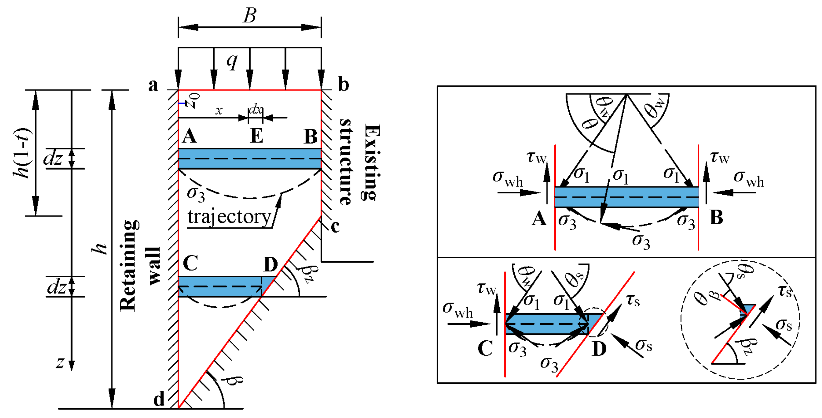
For soil of limited width, there are two kinds of horizontal soil strips between the retaining wall and the existing underground structure. AB is the horizontal soil strip from the retaining wall to the side wall of existing underground structure, and CD is the horizontal soil strip from the retaining wall to the soil slip surface. AB and CD with an extremely small thickness dz are shown in Figure 2, which are behind the retaining wall at an arbitrary burial depth z. AB disappears for semi-infinite soil or when the slip surface does not intersect the existing structure. The width of AB is B and the width of CD depends on the slip surface shape and its position. And they can be expressed by the superposition of the inclined angle β of the slip surface.

The parameter t in Figure 2 indicates the ratio of limited soil width. t equals to Btanβ/h when the slip surface is a plane, in which β is the slip surface angle with respect to the horizontal, and h is the depth of retaining wall. β_z equals to β when the slip surface is a plane. However, β_z changes with the burial depth z when the slip surface is curved. In this case, t needs to be calculated using the integral of cotβ_z. This study mainly focuses on 0 ≤ t ≤ 1.

As the distance x of an arbitrary point E on the horizontal soil strip AB or CD from the retaining wall increases, the angle between the principal stress direction and the horizontal direction θ gradually increases from θ_w at the retaining wall surface (point A and C) to 90°. Then it gradually decreases to θ_w at the existing side wall at point B because of the same soil-wall friction angle with the retaining wall. When x tends to B, θ tends to θ_s for horizontal soil strip CD. θ_s equals to θ_w to make the integral of the horizontal shear stress to be 0.

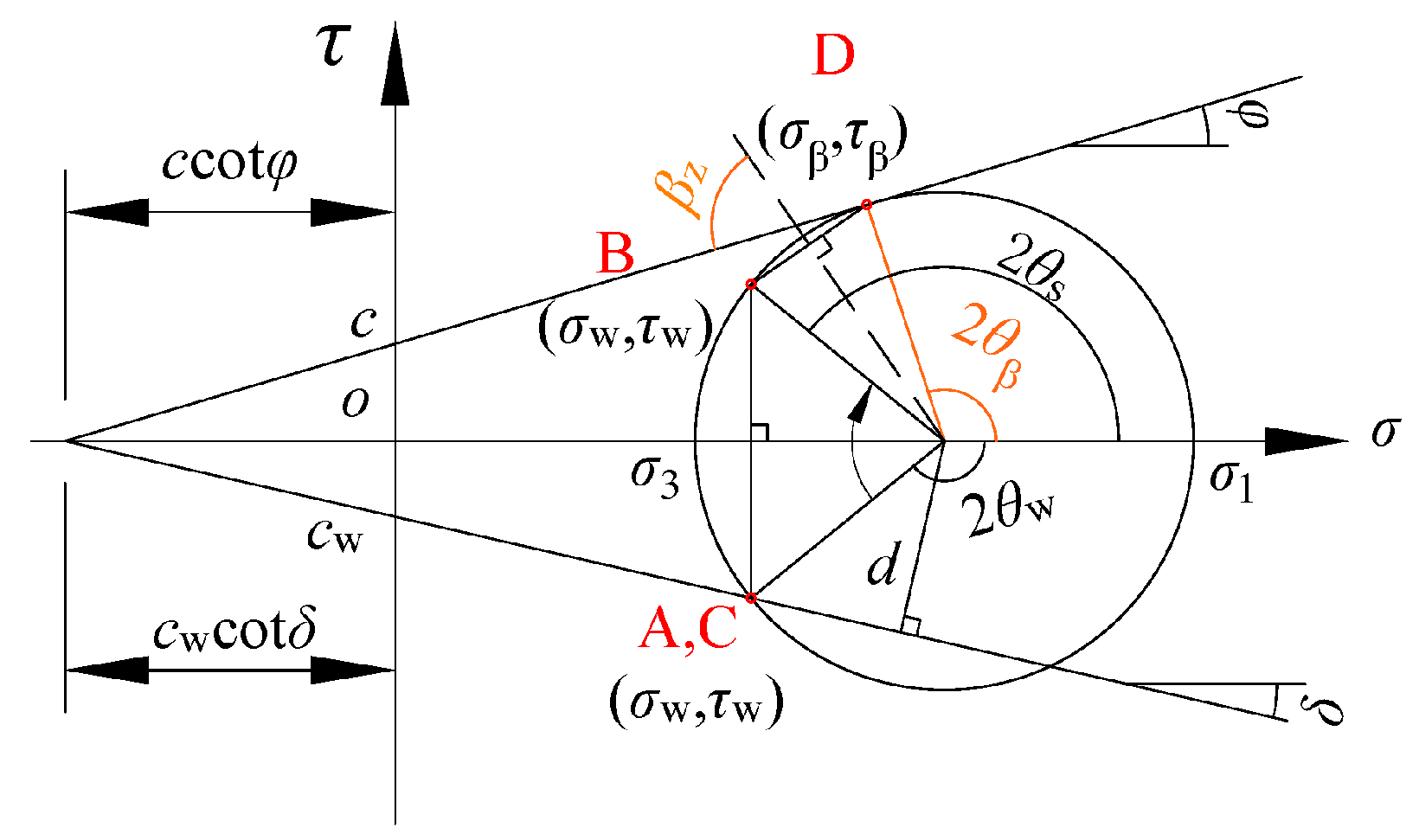
The analysis of any point E on the horizontal soil strip AB and CD using the Mohr stress circle was implemented, as shown in Figure 3. The stresses σ and τ also transform gradually from A to B and from C to D, respectively. There is an angle of θ_β between the principal stress direction and the vertical of slip surface at the active state. θ_β equals to (π/4+φ/2) according to the Mohr stress circle analysis. From Figure 2 we can obtain that θ_s − θ_β = π/2 − β_z.

σ₁ (σ₁ = γz + q) and σ₃ (σ₃ = K_aσ₁) are separately the major and the minor principal stress in Figure 2 and Figure 3, where γ is the soil saturated unit weight, q is the ground surface overload, K_a is the coefficient of the active earth pressure, and φ is the soil internal friction angle. The deflection angle of the minor principal stress direction θ_w at depth z of the c-φ soil is deduced from Figure 3 as:

$${\theta }_w=\frac{\pi }{2}+\frac{\delta }{2}-\frac{1}{2}\arcsin \frac{\sin \delta \left[\gamma z+q-c\cos \phi +c_w\cot \delta \left(1+\sin \phi \right)\right]}{\sin \phi \left(\gamma z+q+c\cot \phi \right)},$$

(1)

where c is the soil cohesion, c_w is the soil-wall cohesion, and δ is the soil-wall friction angle. When δ = 0, θ_w is equal to π/2, and the soil arching effect disappears. In general, if c_wcotδ = ccotφ, then θ_w = [π + δ − arcsin(sinδ/sinφ)]/2, which is consistent with Rao’s [26] results.

According to Figure 3 and Equation (1), the slip surface angle β of c-φ soil at depth z of horizontal soil strip CD is

$${\beta }_z=\frac{\pi }{4}+\frac{\phi -\delta }{2}+\frac{1}{2}\arcsin \frac{\sin \delta \left[\left(\gamma z+q\right)-c\cos \phi +c_w\cot \delta \left(1+\sin \phi \right)\right]}{\sin \phi \left(\gamma z+q+c\cot \phi \right)},$$

(2)

thus, β_z is not affected by B, but increases with increasing γ, q, and φ. β_z is a function of φ and δ and the slip surface is a plane when c_w = ccotφ/cotδ. β_z is equal to (π/4 + φ/2) when δ = 0, which is consistent with Rankine’s slip surface angle, and the soil arching effect disappears. Furthermore, β_z is φ/2 and the slip surface coincide with the retaining wall when δ = φ.

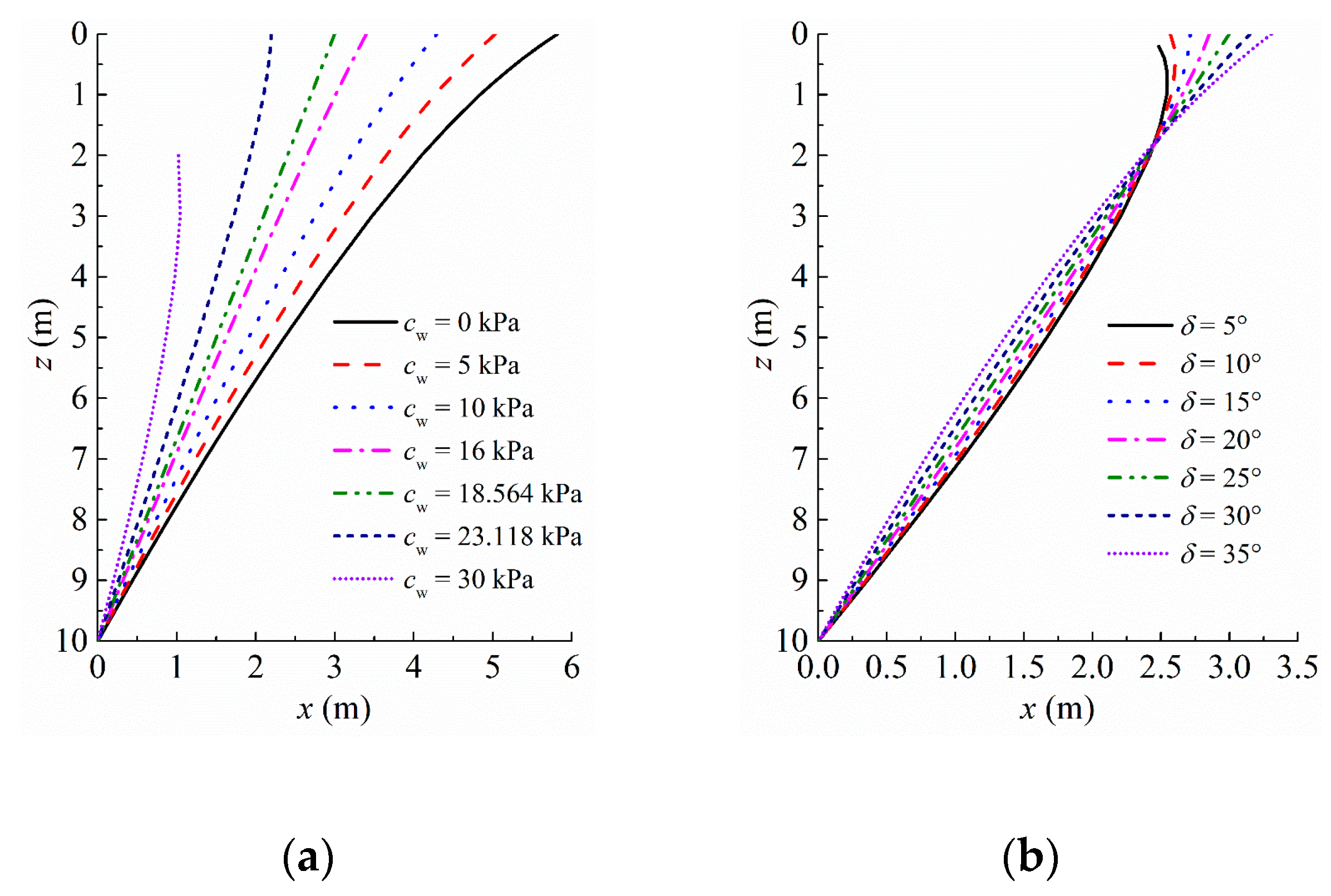
The relationship between c_w and δ are discussed to get clear the soil-wall interaction mechanism. Here we assume that c_w and δ are independent from each other; thus, the influence of c_w and δ on β is shown in Figure 4a,b, respectively, in which γ = 19 kN/m³, q = 0, φ = 37°, δ = 25°, and c = 30 kPa, then c × cotφ/cotδ = 18.564 kPa. When β = 90°, c_w = 23.118 kPa. Comparison of Figure 4a,b, it shows that the influence of δ on the curvature of the slip surface can offset the effect of c_w and β independents of z. Then the slip surface is a plane, such as c_w = 18.564 kPa in Figure 4a and δ = 25° in Figure 4b.

For the limit equilibrium method of a horizontal soil strip, the horizontal force is not disturbed when the burial depth z is deeper than the wall depth h. After this, the slip surface needs to pass through the wall toe. Furthermore, when c_wcotδ = ccotφ, the double-fold line slip surface for limited soil is a plane passing through the wall toe and intersecting the side wall of the existing underground structure, then till the ground surface along the existing wall. The inclination angle of the double-fold line slip surface for the limited c-φ soil can be simplified as:

$$\beta =\{\begin{array}{l}\frac{\pi }{2}\hspace{1em}\hspace{1em}\hspace{1em}\hspace{1em}\hspace{1em}\hspace{1em}\hspace{1em}\hspace{1em};\left(0\le z\le \left(h-B\tan \beta \right)\right)\\ \frac{\pi }{4}+\frac{\phi -\delta }{2}+\frac{1}{2}\arcsin \frac{\sin \delta }{\sin \phi };\left(\left(h-B\tan \beta \right)<z\le h\right)\end{array}.$$

(3)

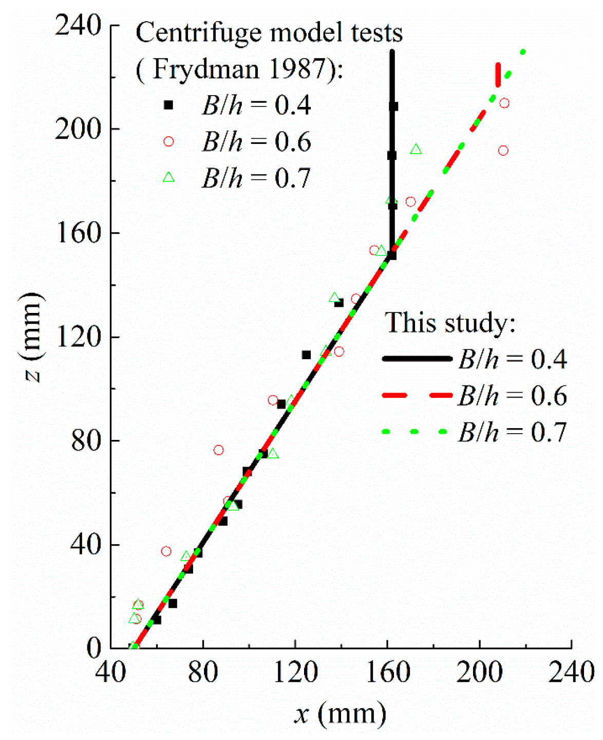
Figure 5 shows the comparison of the double-fold line slip surface from Equation (3) with the results obtained from centrifuge model tests [6]. The results of this study are consistent with those obtained from centrifuge model tests. Therefore, by setting c_w = c × tanδ/tanφ, the soil-wall interaction can be determined by δ and the calculation of active earth pressure distribution based on the slip surface is simplified. c_w = c × tanδ/tanφ is assumed in the following calculation procedure.

2.3. Soil Arching Analysis

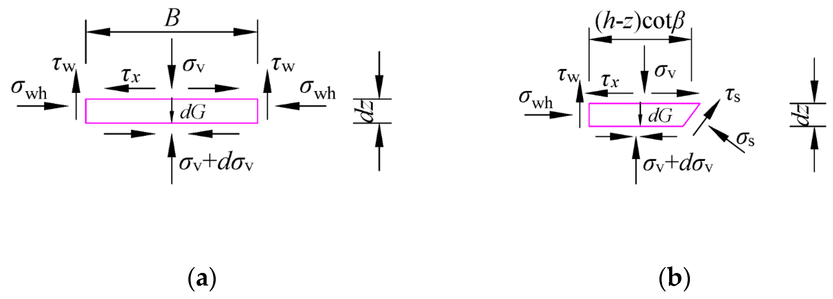
Based on the above research, the trapezoidal limited c-φ soil slip wedge and the stresses acting on the horizontal soil strip at depth z are shown in Figure 2. The soil slip wedge is surrounded by the red lines delimiting the ground surface ab, the existing side wall segment bc, the slip surface segment cd, and the retaining wall segment ad. The external forces acting on the horizontal soil strip within the slip wedge are the horizontal normal stress σ_wh and shear stress τ_w near the retaining wall and the existing side wall; the vertical stress σ_s and shear stress τ_s near the slip surface cd; and the vertical stress σ_v and (σ_v + dσ_v) and shear stress τ_x and (τ_x + dτ_x) above and below the horizontal soil strip, respectively. Based on the Mohr stress circle analysis as shown in Figure 3, the stresses at any distance x from the retaining wall within the slip wedge are deduced as:

$$\{\begin{array}{l}{\sigma }_h=\left(\frac{1+\cos 2\theta \sin \phi }{1+\sin \phi }\right)\left({\sigma }_1+c\cot \phi \right)-c\cot \phi \\ {\sigma }_v=\left(\frac{1-\cos 2\theta \sin \phi }{1+\sin \phi }\right)\left({\sigma }_1+c\cot \phi \right)-c\cot \phi \\ {\tau }_x=\frac{\sin 2\theta \sin \phi }{1+\sin \phi }\left({\sigma }_1+c\cot \phi \right)\end{array},$$

(4)

in which θ corresponds to x. Equation (4) corresponds to the stress state at the wall surface (points A, B, C) when θ = θ_w, whereas it corresponds to the stress state at soil slip surface (point D) when θ = θ_s. The ranges of θ for soil strips AB and CD are [θ_w, π − θ_w] and [θ_w, π − θ_s], respectively.

In order to satisfy the shear stress integral of the horizontal soil strip to be zero within the slip wedge, i.e., ${\displaystyle {\int }_{-B_z/2}^{B_z/2}\tau \left(x\right)dx}=0$, the stress arch of the horizontal soil strip must be bilaterally symmetric, in which B_z is the soil width at depth z. B_z = B when 0 ≤ z ≤ (h-Btanβ), and the stress arch is identical everywhere. However, B_z = (h-z) cotβ when (h-Btanβ) < z ≤ h, and the arc length decreases as the burial depth increases. The stress state of the horizontal soil strip, in the active state, is like that of an inverted arch. In order to satisfy the self-support of the inverted arch, and the traits unchanged after compressing or stretching [17,48,49], the symmetric catenary curve is proposed to describe the stress arc of limited soil in active state and its mathematical expression is:

$$y=\frac{a}{2}\left[\exp \left(\frac{x}{a}\right)+\exp \left(-\frac{x}{a}\right)-\exp \left(\frac{B_z}{2a}\right)-\exp \left(-\frac{B_z}{2a}\right)\right]\left(-\frac{B_z}{2}\le x\le \frac{B_z}{2}\right),$$

(5)

where B_z is the horizontal soil strip width at depth z, a is the undetermined coefficient, which indicates the size of the catenary opening and is a positive value in the active state, and x is the horizontal distance from the vertex. When x = -B_z/2, y’ (x = -B_z/2) = -cotθ_w, and thus:

$$a=\frac{B_z}{2\ln \left(\cot {\theta }_w+\sqrt{{\cot }^2{\theta }_w+1}\right)},$$

(6)

$$\cot \theta =-\frac{1}{2}\left[\exp \left(\frac{x}{a}\right)-\exp \left(-\frac{x}{a}\right)\right].$$

(7)

The stress values at any position on the horizontal soil strip within the slip wedge can be obtained by substituting Equation (7) into Equation (4), which is represented by a symmetric catenary arch curve.

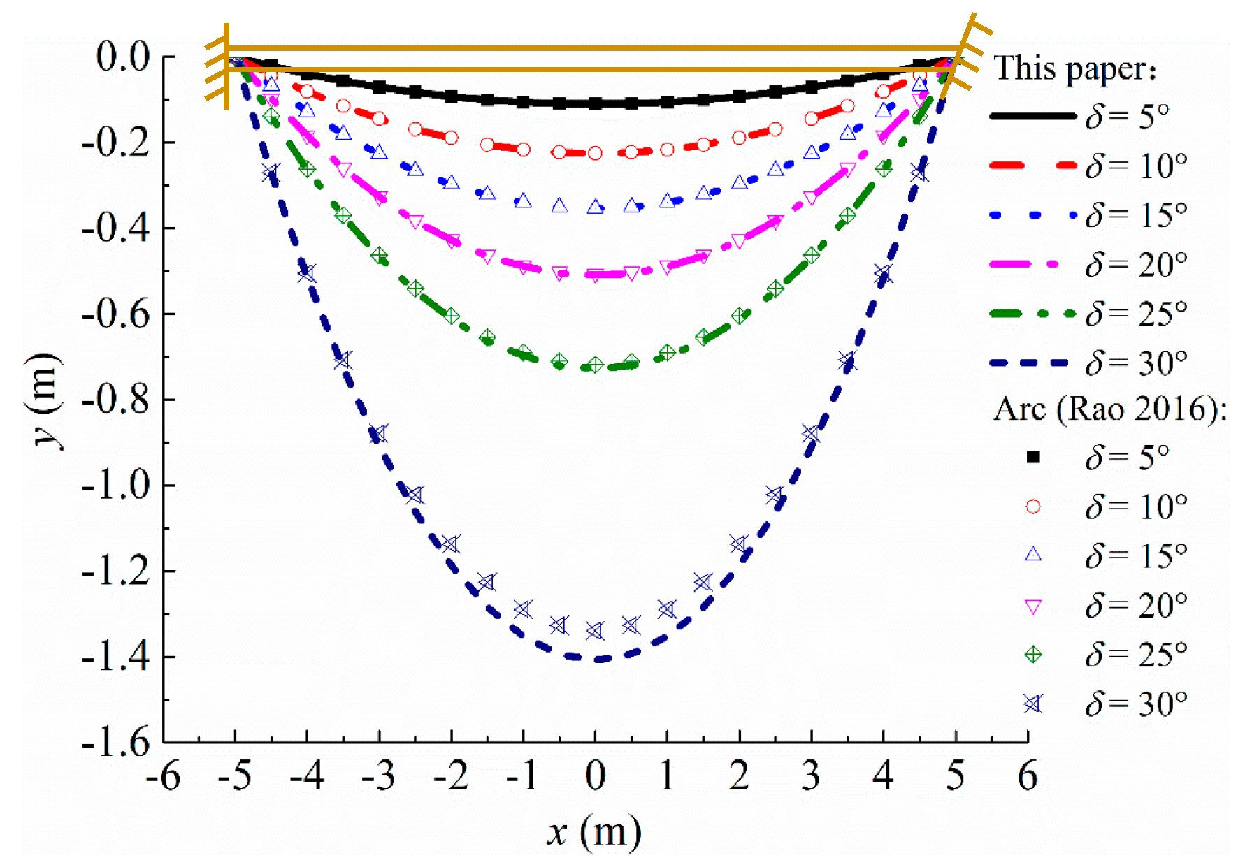
The comparison between the catenary arching curve in Equation (5) and the arc arching curve obtained by Rao [26] is shown in Figure 6, in which φ is 30° and B is 10 m. As can be seen, the curvature of the arch curve increases with increasing δ, and the curvature of the catenary arch is larger. The results from the catenary curve tend to be consistent with the arc when δ is small. The larger δ, the more obvious the difference becomes.

2.4. Lateral Active Earth Pressure Coefficient

The lateral active earth pressure coefficient K_aw is the key to calculating the active earth pressure. The soil arching effect, which deflects the stress trajectory direction, has a significant influence on K_aw. The average vertical stress of the horizontal soil strip $\overline{{\sigma }_v}$ calculated from the catenary arching curve obtained in Section 2.3 is:

$$\overline{{\sigma }_v}=\frac{{\displaystyle \underset{-B_z/2}{\overset{0}{\int }}{\sigma }_v}dx}{B_z/2}=\frac{\gamma z+q+c\cot \phi }{1+\sin \phi }\left(1-\sin \phi -4\sin \phi \frac{a}{B_z}\frac{1-\exp \left(\frac{B_z}{a}\right)}{1+\exp \left(\frac{B_z}{a}\right)}\right)-c\cot \phi .$$

(8)

When δ = 0, $\overline{{\sigma }_v}=\gamma z+q$. Thus, the lateral active earth pressure coefficient K_aw is:

$$K_{aw}=\frac{{\sigma }_{wh}}{\overline{{\sigma }_v}}=\frac{\frac{\gamma z+q+c\cot \phi }{1+\sin \phi }\left(1+\sin \phi \left(1-\frac{8\exp \left(-\frac{B_z}{a}\right)}{{\left(\exp \left(-\frac{B_z}{a}\right)+1\right)}^2}\right)\right)-c\cot \phi }{\frac{\gamma z+q+c\cot \phi }{1+\sin \phi }\left(1-\sin \phi \left(1+\frac{4a}{B_z}\frac{\exp \left(-\frac{B_z}{a}\right)-1}{\exp \left(-\frac{B_z}{a}\right)+1}\right)\right)-c\cot \phi }.$$

(9)

It is the general expression of K_aw obtained by considering the influence of soil cohesion. K_aw = f (c, φ, δ, γ, z, q) and is non-linearly distributed along the wall depth. When δ = 0, $K_{aw}=\frac{1-\sin \phi }{1+\sin \phi }-\frac{2c\cot \phi }{\gamma z+q}\frac{\sin \phi }{1+\sin \phi }$. When φ = 0, K_aw = 1 − 2c/(γz + q), which is the earth pressure coefficient under static conditions. When c = δ = 0, K_aw = K_a. Since (B_z/a) is only a function of θ_w, K_aw is not affected by the presence of limited c-φ soil width.

2.5. Active Earth Pressure Distribution

The lateral active earth pressure coefficient K_aw obtained in Equation (9) by considering the influence of soil cohesion c is a function of the burial depth z. Thus, K_aw must be synchronously integrated when the limit equilibrium method of the horizontal soil strip is used to raise the active earth pressure model and makes the calculation process more complicated. To simplify the calculation process, the coordinate translation method is used to convert K_aw of the cohesion soil into the K_aw’ of sandy soil. From Figure 3 we know that $\left(K_{aw}\overline{{\sigma }_v}+c\cot \phi \right)=\left(\overline{{\sigma }_v}+c\cot \phi \right)K_{aw}{}^{\prime }$, and thus:

$$K_{aw}{}^{\prime }=\frac{{\sigma }_{wh}{}^{\prime }}{\overline{{\sigma }_v}{}^{\prime }}=\frac{{\sigma }_{wh}+c\cot \phi }{\overline{{\sigma }_v}+c\cot \phi }=\frac{1+\sin \phi \frac{\exp \left(-\frac{B_z}{a}\right)+\exp \left(\frac{B_z}{a}\right)-6}{\exp \left(-\frac{B_z}{a}\right)+\exp \left(\frac{B_z}{a}\right)+2}}{1-\sin \phi \left(1+\frac{4a}{B_z}\frac{1-\exp \left(\frac{B_z}{a}\right)}{1+\exp \left(\frac{B_z}{a}\right)}\right)},$$

(10)

K_aw’ is independent from z.

B is in the range of (0, hcotβ) when the existing large rigid underground structure is in the influence range of the retaining wall, and the soil width is limited. The refined boundary of the c-φ soil limited width will be discussed later. The horizontal soil strip of the limited c-φ soil behind the retaining wall can be divided into two main parts along the wall depth: the rectangular region (case1) in which (0 ≤ z ≤ (h-Btanβ)), and the trapezoidal region (case2) in which ((h-Btanβ) < z ≤ h), as shown in Figure 7a,b. The saturated weight of the horizontal soil strip is dG.

2.5.1. Case1: 0 ≤ z ≤ (h-Btanβ)

From the stress equilibrium of the horizontal soil strip in the rectangular region in Figure 7a, we can obtain that

$$\gamma =\frac{d\overline{{\sigma }_v{}^{\prime }}}{dz}+\frac{2K_{aw}{}^{\prime }\tan \delta }{B}\overline{{\sigma }_v{}^{\prime }}.$$

(11)

When z = 0, $\overline{{\sigma }_v{}^{\prime }}=q$; thus:

$$\overline{{\sigma }_{v1}{}^{\prime }}=\left(q-\frac{\gamma }{\eta }\right)e^{-\eta z}+\frac{\gamma }{\eta },$$

(12)

where $\eta =\frac{2K_{aw}{}^{\prime }\tan \delta }{B}$. When δ = 0, $\overline{{\sigma }_{v1}{}^{\prime }}=q+\gamma z$.

Thus, when 0 ≤ z ≤ (h-Btanβ), the active earth pressure for the limited c-φ soil is:

$${\sigma }_{wh1}=K_{aw}{}^{\prime }\left[\left(q-\frac{\gamma }{\eta }\right)e^{-\eta z}+\frac{\gamma }{\eta }\right]-c\cot \phi .$$

(13)

When q = c = 0, ${\sigma }_{wh1}=\frac{\gamma B}{2\tan \delta }\left(1-\exp \left(-\frac{2K_{aw}{}^{\prime }\tan \delta }{B}z\right)\right)$, which is consistent with Handy’s [17] results, except for the lateral active earth pressure coefficient.

2.5.2. Case2: (h-Btanβ) < z ≤ h

From the horizontal and vertical stress equilibrium of the horizontal soil strip in the trapezoidal region in Figure 7b, we can obtain that:

$$\frac{d\overline{{\sigma }_v{}^{\prime }}}{dz}=\gamma +\frac{1}{h-z}\left(\overline{{\sigma }_v{}^{\prime }}-{\sigma }_s{}^{\prime }-\frac{{\tau }_w{}^{\prime }+{\tau }_s{}^{\prime }}{\cot \beta }\right),$$

(14)

$${\sigma }_{wh}{}^{\prime }+{\tau }_s{}^{\prime }\cot \beta -{\sigma }_s{}^{\prime }=0.$$

(15)

When B > hcotβ, case1 is negligible and (h-Btanβ) = (1-t) h = 0. Otherwise, 0 < t < 1, and $\overline{{\sigma }_{v2}{}^{\prime }}\left(z=\left(1-t\right)h\right)=\overline{{\sigma }_{v1}{}^{\prime }}\left(z=\left(1-t\right)h\right)=\left(q-\frac{\gamma }{\eta }\right)e^{-\eta \left(1-t\right)h}+\frac{\gamma }{\eta }$. Thus:

$$\overline{{\sigma }_{v2}{}^{\prime }}=\left[\left(q-\frac{\gamma }{\eta }\right)e^{-\eta \left(1-t\right)h}+\frac{\gamma }{\eta }+\frac{\gamma th}{2-\chi K_{aw}{}^{\prime }}\right]{\left(\frac{h-z}{th}\right)}^{\chi K_{aw}{}^{\prime }-1}-\frac{\gamma \left(h-z\right)}{\left(2-\chi K_{aw}{}^{\prime }\right)},$$

(16)

where $\chi =\frac{\tan \beta \cos \left(\beta -\phi -\delta \right)}{\cos \delta \sin \left(\beta -\phi \right)}$.

When (h-Btanβ) < z ≤ h, the active earth pressure for the limited c-φ soil is:

$${\sigma }_{wh2}=K_{aw}{}^{\prime }\left[\left[\left(q-\frac{\gamma }{\eta }\right)e^{-\eta \left(1-t\right)h}+\frac{\gamma }{\eta }+\frac{\gamma th}{2-\chi K_{aw}{}^{\prime }}\right]{\left(\frac{h-z}{th}\right)}^{\chi K_{aw}{}^{\prime }-1}-\frac{\gamma \left(h-z\right)}{\left(2-\chi K_{aw}{}^{\prime }\right)}\right]-c\cot \phi .$$

(17)

When δ = 0, ${\sigma }_{wh}=K_a\left(q+\gamma z\right)-c\cot \phi$.

Equations (13) and (17) form the calculate model for the active earth pressure distribution of limited c-φ soil between a deep retaining wall and a large rigid underground structure in this study. It is also suitable for a semi-infinite c-φ soil (t = 1).

2.6. Tension Crack Depth in the Top Wall

There are tension cracks within a certain depth z₀ near the top of wall for a c-φ soil in active state. This indicates that the soil in this depth (0 < z < z₀) is separated from the back of retaining wall and then σ_wh = 0. When σ_wh = 0 in Equation (13), the burial depth z₀ is:

$$z_0=-\frac{B}{2K_{aw}{}^{\prime }\tan \delta }\ln \frac{c\cot \phi \tan \delta -\gamma B/2}{q{K}_{aw}{}^{\prime }\tan \delta -\gamma B/2}.$$

(18)

Equation (18) shows that z₀ is affected by B, c, φ, δ, γ and q. z₀ increases as c and B increase, but decreases as increasing φ, δ and q. $z_0=\frac{c\cot \phi }{\gamma }\frac{1+\sin \phi }{1-\sin \phi }-\frac{q}{\gamma }$ while δ = 0. Furthermore $z_0=2c/\left(\gamma \sqrt{K_a}\right)$ while δ = 0 and q = 0; this is consistent with the classical Rankine method [1].

2.7. Boundary Values of the Limited Width

Due to the ground surface overload q, z₀ may not necessarily occur in the active state. In this case, z₀ must be analyzed additionally. According to Equation (18), when z₀ < 0, z₀ = 0. When z₀ > 0, $0\le \frac{c\cot \phi \tan \delta -\gamma B/2}{q{K}_{aw}{}^{\prime }\tan \delta -\gamma B/2}\le 1$. Thus, $B\ge \frac{2c\cot \phi }{\gamma \cot \delta }$, while ccotφ ≥ qK_aw’. However, $B\le \frac{2c\cot \phi }{\gamma \cot \delta }$ while ccotφ < qK_aw’. Therefore, the boundary for c-φ soil limited width B is:

$$\{\begin{array}{l}\frac{2c\cot \phi }{\gamma \cot \delta }\le B\le h\cot \beta \left(\mathrm{when} c\cot \phi \ge K_{aw}{}^{\prime }q\right)\\ B\le \frac{2c\cot \phi }{\gamma \cot \delta } \mathrm{and} B\le h\cot \beta \left(\mathrm{when} c\cot \phi <K_{aw}{}^{\prime }q\right)\end{array}.$$

(19)

Otherwise, the c-φ soil width is semi-infinite or beyond the calculation scope of this study for B < 2ccotφ/(γcotδ) while ccotφ ≥ qK_aw’.

2.8. Resultant Force and Its Action Point

From the integral of Equations (13) and (17), the horizontal component of active earth pressure resultant force acting on the retaining wall E_wh is:

$$E_{wh}={\displaystyle \underset{z_0}{\overset{h-B\tan \beta }{\int }}{\sigma }_{wh1}dz}+{\displaystyle \underset{h-B\tan \beta }{\overset{h}{\int }}{\sigma }_{wh2}dz}.$$

(20)

The action point of the resultant force h_w is:

$$h_w=\frac{{\displaystyle \underset{z_0}{\overset{h-B\tan \beta }{\int }}{\sigma }_{wh1}\left(h-z\right)dz}+{\displaystyle \underset{h-B\tan \beta }{\overset{h}{\int }}{\sigma }_{wh2}\left(h-z\right)dz}}{E_{wh}}.$$

(21)

When δ = 0:

$$E_{wh}=\frac{1-\sin \phi }{1+\sin \phi }\left(q\left(h-z_0\right)+\gamma \left(h^2-z_0{}^2\right)/2\right)-c\cot \phi \left(h-z_0\right),$$

(22)

$$h_w=\frac{\frac{1-\sin \phi }{1+\sin \phi }\left[q{\left(h-z_0\right)}^2/2+\gamma h\left(h^2-z_0{}^2\right)/2-\gamma \left(h^3-z_0{}^3\right)/3\right]-c\cot \phi \frac{{\left(h-z_0\right)}^2}{2}}{\frac{1-\sin \phi }{1+\sin \phi }\left[q\left(h-z_0\right)+\gamma \left(h^2-z_0{}^2\right)/2\right]-c\cot \phi \left(h-z_0\right)}.$$

(23)

Furthermore, when c = 0, $E_{wh}=\frac{1-\sin \phi }{1+\sin \phi }\left(qh+\frac{\gamma h^2}{2}\right)$ and $h_w=\frac{h}{3}\frac{\gamma h+3q}{\gamma h+2q}$; and when c = q = 0, $E_{wh}=\frac{1-\sin \phi }{1+\sin \phi }\frac{\gamma h^2}{2}$ and $h_w=\frac{h}{3}$, which is coincident with Rankine’s solution [1].

3. Comparison and Verification

3.1. Numerical Analysis

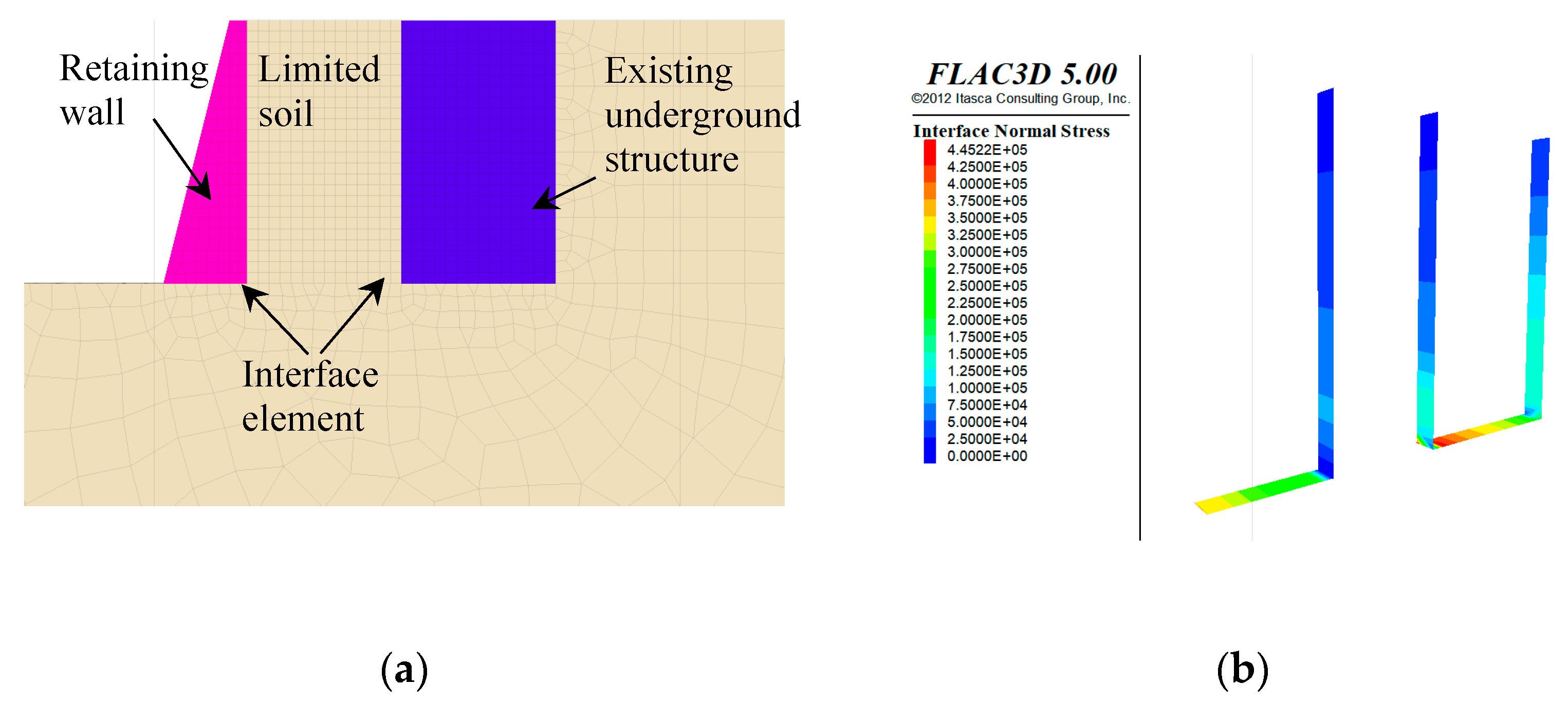
A numerical simulation method was used to clarify the limited c-φ soil mechanism between a deep retaining wall and an existing large rigid underground structure. The finite difference numerical analysis model established in FLAC3D (Fast Lagrangian Analysis of three-dimensional Continua) [50,51,52,53] is shown in Figure 8. In which the boundary conditions are: the thickness of the mesh was only 1 m in order to simulate the plane strain state; the depth of the mesh, and the width at the right side of the large rigid underground structure was four times the retaining wall depth [13]. The bottom of the mesh was fixed; the surrounding side can slide vertically; and the top surface was free.

The burial depth of the large rigid existing underground structure and of the retaining wall were both 12 m. The width between the retaining wall and the existing wall was determined by the limited soil width, which were separately 1, 2, 4, 6, and 8 m. The thickness of the retaining wall was 0.8 m at the top and 3.8 m at the bottom. Its back in contact with soil was vertical. The soil-wall interaction was simulated using an interface element (the rigidness of the interface element was 10 times that of the soil rigidness), and the constitutive model was used the Coulomb shear model. The c-φ soil was simulated using a Mohr Coulomb model (γ = 24.5 kN/m³; E = 15 MPa; μ = 0.35; c = 30 kPa; φ = 25°). The simulation was carried out for both the retaining structure and the existing large rigid underground structure using an elastic element (μ = 0.2; γ = 30 kN/m³; E = 35 GPa), where E was the soil elastic modulus, and μ was the Poisson’s ratio. The min and max limited soil width were separately 0.76 and 6.04 m, according to Equation (19).

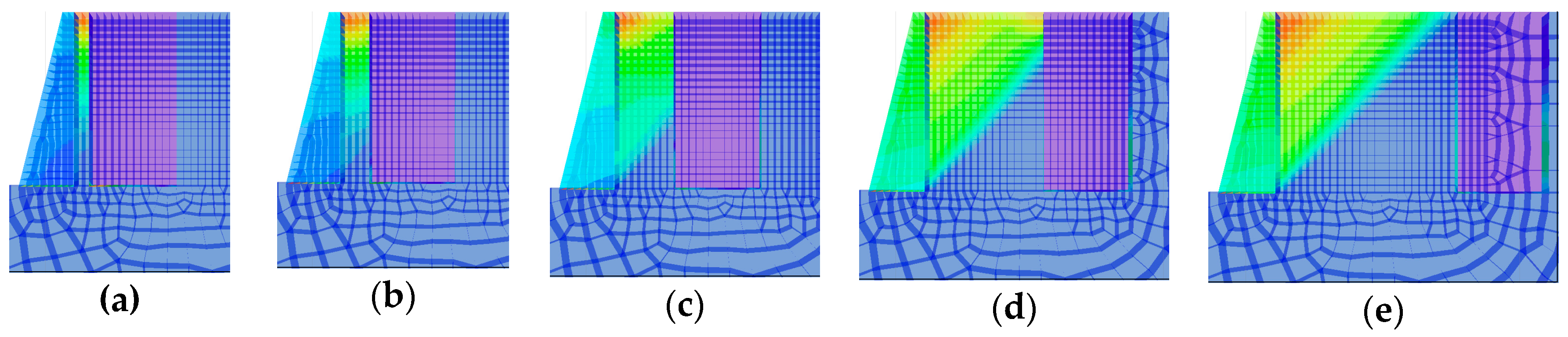
Generally, the retaining wall displacement which forces the soil into the active state is about 0.2 × 10⁻² h, in which h is the retaining wall depth [54]. By giving a leftward displacement of about 24 mm to the retaining wall, the calculated cloud map of displacement for different limited c-φ soil width is shown in Figure 9. The slope of the inclined plane is approximately the same for all the cases. The inclined plane intersects the side wall of the existing large rigid underground structure when the limited c-φ soil width is less than 6.04 m. The results verify that the theoretical result for the double-fold line slip surface of the limited c-φ soil obtained in Equation (3) is reasonable.

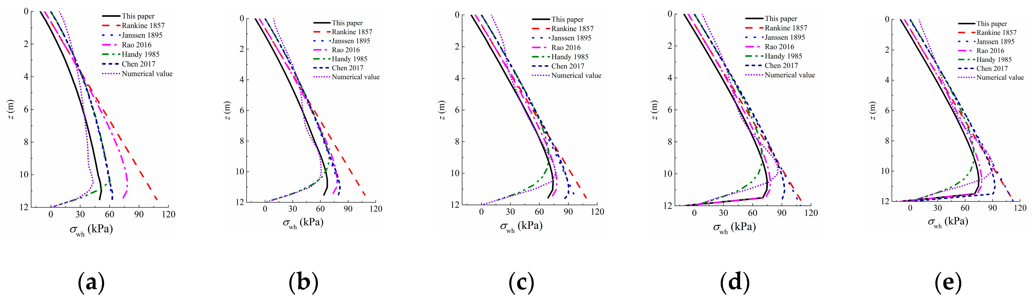
The numerical results of the active earth pressure distribution were obtained for B/h of 0.083, 0.167, 0.333, 0.500, and 0.667, as shown in Figure 10. The results are also compared with the theoretical results obtained in this study and by other scholars. The distribution of the active earth pressure is large in the middle and small at both ends. The active earth pressure decreases as the decreasing of limited soil width in the numerical results and this study. The numerical results are close to the values both from this study and other scholars when the limited soil width is large. However, it is closer to the results by this study when the limited soil width is small. This demonstrates that the theory developed in this study reflects the actual situation well.

3.2. Centrifuge Model Tests

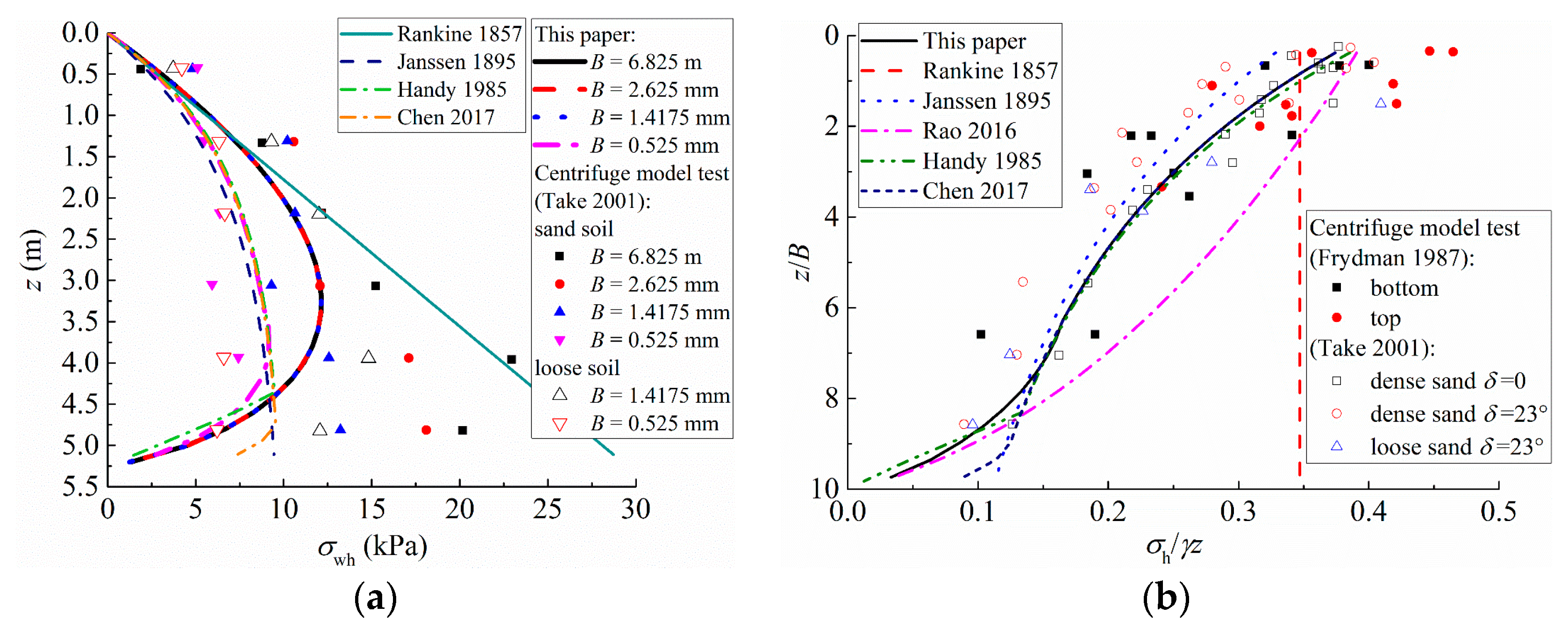
The results of the active earth pressure distribution and its standard values for c-φ soil of limited width were compared with the centrifuge model test results of Frydman and Keissar (1987) [6] and of Take and Valsangkar (2001) [7]. They were also compared with the theoretical results of multiple scholars, as shown in Figure 11. The parameters are the same as those used in Take’s (2001) [7] centrifuge model tests, i.e., γ = 16.2 kN/m³, q = c = 0, φ = 29°, δ = 23°, h = 5.25 m (equals to 140 mm on the centrifuge model scale), and B = 0.525 m, 1.4175 m, 2.625 m, and 6.825 m.

The maximum width of limited soil is 1.421 m according to Equation (19). The soil width set by the centrifuge model tests exceed the maximum boundary of limited soil width in this study except for B = 0.525 m and 1.4175 m. However, B = 1.4175 m is like the max limited soil width 1.421 m. the active earth pressure distribution is shown in Figure 11a. The black, red, and blue lines in Figure 11a are almost overlapped because they represent the active earth pressure for B = 6.825 m, 2.625 m, and 1.4175 m.

Figure 11b gives out the normalized active earth pressure distribution, which is obtained through standardizing the active earth pressure σ_h with the vertical gravity stress γz and standardizing the burial depth z with the limited soil width B. By comparing the theoretical results with those of other scholars, it shows that the results obtained in this study are almost the same as the solution by Handy (1985) [17] and Chen (2017) [19] when the burial depth is small. However, Handy’s (1985) [17] and Chen’s (2017) [19] solution does not transit from top to bottom smoothly and Chen’s (2017) [19] solution overrated σ_wh while the burial depth is large. Although the soil cohesion is considered in Rao’s (2016) [26] method, the influence of the limited width cannot be considered. Both soil cohesion and the limited width are considered in this study. Figure 11 shows that the results in this study are the closest to the results of centrifuge model tests by comparing with the results of other theoretical methods.

4. Parametric Study

The active earth pressure distribution, as well as the resultant force and its action point, are key controlling factors in the design of a deep retaining structure. In this study, it can be found that the main influencing factors are the soil cohesion c, the ground surface overload q, the wall depth h, the distance between the retaining wall and the existing large rigid underground structure B, the soil internal friction angle φ, and the soil-wall friction angle δ. Unless otherwise stated, the parameters used in the following computations are γ = 15.8 kN/m³; h = 8.5 m; q = 0 kPa; c = 0 kPa; φ = 36°; δ = 25°; and B = 1 m, which are consistent with Fan’s (2010) [13] numerical simulation. In this case, the factor of the limited width of c-φ soil is t = 0.4. The boundary value for the maximum limited c-φ soil width is B_max = 2.52 m; and the maximum soil cohesion is 12.3 kPa when B = 1 m according to the above calculation parameters.

4.1. Soil Internal Griction Angle and Soil-Wall Friction Angle

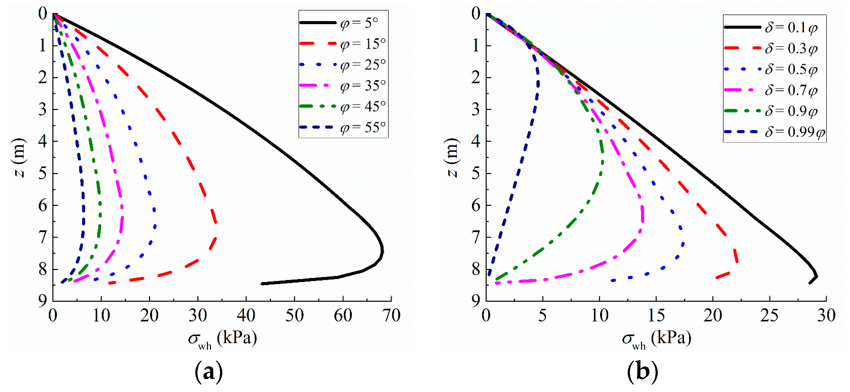
The influence of the soil inner friction angle φ and the soil-wall friction angle δ on the active earth pressure distribution σ_wh according to Equations (13) and (17) is shown in Figure 12. Different values of φ varying from 5° to 55° and different values of δ varying from 3.6° to 35.64° were used. σ_wh and B_max decrease as φ and δ increase. The burial depth of the maximum active earth pressure increases significantly with increasing δ. This indicates that increasing the wall friction can reduce the active earth pressure acting on the wall.

4.2. Soil Cohesion and Ground Surface Overload

The influence of soil cohesion c and the ground surface overload q on the active earth pressure distribution σ_wh is shown in Figure 13. Both of c and q vary from 0 to 25 kPa. σ_wh decreases with increasing c. σ_wh increases with increasing q when the burial depth is small. It is worth noting that a larger soil cohesion may lead to tensile stress of the active earth pressure behind the retaining wall, which will affect the overall stability of the deep retaining wall. According to Equation (19), the soil width in Figure 13b all exceed the boundary value of the maximum limited soil width. That is, the calculation results are based on a semi-infinite soil. The burial depth of the maximum active earth pressure increases with increasing q. Figure 13b shows that it is necessary to implement larger reinforcement measures within the top half of the retaining wall when the ground surface is overloaded.

4.3. Soil’s Limited Width and Wall Height

The influence of the spatial effect of the limited soil width B and the wall height h on the active earth pressure distribution σ_wh is shown in Figure 14, in which B vary from 0.4 to 1.9 m and h vary from 1 to 10 m. σ_wh increases with increasing B and h. The smaller the limited soil width, the greater its impact on the active earth pressure distribution. σ_wh cannot be solved using the method developed in this study when B is less than the minimum width calculated using Equation (19). The boundary value for the maximum limited soil width increases with increasing wall depth.

4.4. Comparison after Normalization

In order to compare the effects of each parameter (φ, δ, c, q, B, h) in Figure 12, Figure 13, and Figure 14, this study standardized the parameters to i, the ratio of the difference between the current value and the minimum value of the parameter to the range, that is (current value – minimum value)/(maximum value – minimum value). The standard values of the resultant force (E_wh/(γh²/2)) and its standard action point (h_w/h) calculated according to Equations (20) and (21) change with the parameter i, as shown in Figure 15. (E_wh/(γh²/2)) increases as B and q increase but decreases as c, φ, δ, and h increase. The impacts of the parameter on (E_wh/(γh²/2)) from largest to smallest are as follows: φ, δ, c, B, q, and h. (h_w/h) increases with increasing φ, δ, and q but decreases with increasing B, c, and h. The impacts of the parameters on (h_w/h) from largest to smallest are as follows: c, δ, q, φ, B, and h. Controlling of the key influencing factors, i.e., increasing the soil-wall friction and decreasing the limited soil width (not less than the minimum boundary calculated using Equation (19)), will increase the safety and economic efficiency of the retaining structure in a dense underground environment significantly.

5. Conclusions

In order to obtain the active earth pressure and its action law on the retaining structure under the limited c-φ soil condition, and to clarify the soil-wall interaction mechanism and the limited c-φ soil boundary width when the soil arching effect is significant, the theoretical method on the basis of previous studies was improved in this study. Four main conclusions are summarized as below:

• The effect of soil-wall cohesion can be expressed by the soil-wall friction angle. A double-fold line slip surface that considers the soil internal friction angle and the soil-wall friction angle was determined to be suitable for calculating the active earth pressure of a limited c-φ soil, and a symmetrical catenary arching curve was proposed to simulate the minor principal stress trajectory of a horizontal soil strip.
• An active earth pressure calculation model for a limited c-φ soil that considers ground surface overload was proposed based on the limit equilibrium method of a horizontal soil strip and the improved soil arching effect theory. The model proposed in this study can be simplified into the classic active earth pressure theory, and it reflects the situation for a limited c-φ soil better than other theoretical methods. The laterally active earth pressure coefficient of a limited c-φ soil is a function of burial depth, but it is independent of the limited soil width. The proposed active earth pressure distribution is large in middle and small at both ends, which is consistent with the results of the numerical simulation and the centrifuge model tests.
• An explicit boundary width for a limited c-φ soil during the active earth pressure calculation was determined. When the distance between the existing large rigid underground structure and the retaining wall of the foundation pit is within the boundary of the limited c-φ soil width, the active earth pressure model proposed in this study is needed for the calculation. However, the method proposed in this study is not suitable for situations where B < (2ccotφ)/(γcotδ) and ccotφ ≥ qK_aw’.
• The changes in the active earth pressure due to the limited c-φ soil parameters were obtained. The factors that have the greatest influence on the resultant force and its action point are the soil internal friction angle and the soil cohesion separately. Thus, the influence of soil cohesion cannot be ignored. The smaller of the limited soil width, the more sensitive the active earth pressure to it. Increasing the wall friction and reducing the limited soil width can reduce the active earth pressure acting on the retaining wall. Reinforced measures should be taken on the upper part of the retaining wall when the ground surface is overloaded.

References

- Rankine, W.J.M. On the stability of loose earth. Philos. Trans. R. Soc. Lond. 1857, 147, 9–27. [Google Scholar]
- Aubertin, M.; Li, L.S.T.B.M.; Arnoldi, S.; Belem, T.; Bussière, B.; Benzaazoua, M.; Simon, R. Interaction between backfill and rock mass in narrow stopes. Soil Rock Mech. Am. 2003, 1, 1157–1164. [Google Scholar]
- Li, L.; Aubertin, M.; Belem, T. Formulation of a three dimensional Analytical solution to evaluate stresses in backfilled vertical narrow openings. Can. Geotech. J. 2005, 42, 1705–1717. [Google Scholar] [CrossRef]
- Nishimura, S.; Takahashi, H.; Morikawa, Y. Observations of dynamic and non-dynamic interactions between a quay wall and partially stabilized backfill. Soils Found. 2012, 52, 81–98. [Google Scholar] [CrossRef] [Green Version]
- Janssen, H.A. Experiments about pressures of grain in silos. Z. VDI 1895, 39, 1045–1049. [Google Scholar]
- Frydman, S.; Keissar, I. Earth pressure on retaining walls near rock faces. J. Geotech. Eng. ASCE 1987, 113, 586–599. [Google Scholar] [CrossRef]
- Take, W.A.; Valsangkar, A.J. Earth pressures on unyielding retaining walls of narrow backfill width. Can. Geotech. J. 2001, 38, 1220–1230. [Google Scholar] [CrossRef]
- Troy, S.; Hagerty, D.J. Earth pressures in confined cohesionless backfill against tall rigid walls—A case history. Can. Geotech. J. 2011, 48, 1188–1197. [Google Scholar]
- Khosravi, M.H.; Pipatpongsa, T.; Takemura, J. Experimental analysis of earth pressure against rigid retaining walls under translation mode. Geotechnique 2013, 63, 1020–1028. [Google Scholar] [CrossRef]
- Yang, M.H.; Tang, X.C. Rigid retaining walls with narrow cohesionless backfills under various wall movement modes. Int. J. Geomech. 2017, 17, 04017098. [Google Scholar] [CrossRef]
- Leshchinsky, D.; Hu, Y.; Han, J. Limited reinforced space in segmental retaining walls. Geotext. Geomembr. 2004, 22, 543–553. [Google Scholar] [CrossRef]
- Hsieh, P.G.; Ou, C.Y.; Lin, Y.L. Three-dimensional numerical analysis of deep excavations with cross walls. Acta Geotech. 2013, 8, 33–48. [Google Scholar] [CrossRef]
- Fan, C.C.; Fang, Y.S. Numerical solution of active earth pressures on rigid retaining walls built near rock faces. Comput. Geotech. 2010, 37, 1023–1029. [Google Scholar] [CrossRef]
- Qiu, G.; Grabe, J. Active earth pressure shielding in quay wall constructions: Numerical modeling. Acta Geotech. 2012, 7, 343–355. [Google Scholar] [CrossRef]
- Greco, V. Active thrust on retaining walls of narrow backfill width. Comput. Geotech. 2013, 50, 66–78. [Google Scholar] [CrossRef]
- Greco, V. Analytical solution of seismic pseudo-static active thrust acting on fascia retaining walls. Soil Dyn. Earthq. Eng. 2014, 57, 25–36. [Google Scholar] [CrossRef]
- Handy, R. The arch in soil arching. J. Geotech. Eng. ASCE 1985, 111, 302–318. [Google Scholar] [CrossRef]
- Li, M.G.; Chen, J.J.; Wang, J.H. Arching effect on lateral pressure of confined granular material: Numerical and theoretical analysis. Granul. Matter 2017, 19, 20. [Google Scholar] [CrossRef]
- Chen, J.J.; Li, M.G.; Wang, J.H. Active Earth Pressure against Rigid Retaining Walls Subjected to Confined Cohesionless Soil. Int. J. Geomech. 2017, 17, 06016041. [Google Scholar] [CrossRef]
- Mittal, S.; Garg, K.G.; Saran, S. Analysis and design of retaining wall having reinforced cohesive frictional backfill. Geotech. Geol. Eng. 2006, 24, 499–522. [Google Scholar] [CrossRef]
- Chen, H.T.; Hung, W.Y.; Chang, C.C.; Chen, Y.J.; Lee, C.J. Centrifuge modeling test of a geotextile-reinforced wall with a very wet clayey backfill. Geotext. Geomembr. 2007, 25, 346–359. [Google Scholar] [CrossRef]
- Ahmadabadi, M.; Ghanbari, A. New procedure for active earth pressure calculation in retaining walls with reinforced cohesive frictional backfill. Geotext. Geomembr. 2009, 27, 456–463. [Google Scholar] [CrossRef]
- Shukla, S.J.; Gupta, S.K.; Sivakugan, N. Active earth pressure on retaining wall for c–φ soil backfill under seismic loading conditions. J. Geotech. Geoenviron. Eng. 2009, 135, 690–696. [Google Scholar] [CrossRef]
- Pantelidis, L. The generalized coefficients of earth pressure: A unified approach. Appl. Sci. 2019, 9, 5291. [Google Scholar] [CrossRef] [Green Version]
- Lin, Y.L.; Yang, X.; Yang, G.L.; Li, Y.; Zhao, L.H. A closed-form solution for seismic passive earth pressure behind a retaining wall supporting cohesive–frictional backfill. Acta Geotech. 2016, 12, 1–9. [Google Scholar] [CrossRef]
- Rao, P.; Chen, Q.; Zhou, Y.; Nimbalkar, S.; Chiaro, G. Determination of active earth pressure on rigid retaining wall considering arching effect in cohesive backfill soil. Int. J. Geomech. 2016, 16, 04015082. [Google Scholar] [CrossRef]
- Kim, J.; Barker, M. Effect of live load surcharge on retaining walls and abutments. J. Geotech. Geoenviron. Eng. 2002, 128, 808–813. [Google Scholar] [CrossRef]
- Ghanbari, A.; Taheri, M. An analytical method for calculating active earth pressure in reinforced retaining walls subject to a line surcharge. Geotext. Geomembr. 2012, 34, 1–10. [Google Scholar] [CrossRef]
- Khosravi, M.H.; Pipatpongsa, T.; Takemura, J. Theoretical analysis of earth pressure against rigid retaining walls under translation mode. Soils Found. 2016, 56, 664–675. [Google Scholar] [CrossRef]
- Porbaha, A.; Zhao, A.; Kobayashi, M.; Kishida, T. Upper bound estimate of scaled reinforced soil retaining walls. Geotext. Geomembr. 2000, 18, 403–413. [Google Scholar] [CrossRef]
- Shahgholi, M.; Fakher, A.; Jones, C.J.F.P. Horizontal slice method of analysis. Geotechnique 2001, 51, 881–885. [Google Scholar] [CrossRef]
- Baker, R.; Klein, Y. An integrated limiting equilibrium approach for design of reinforced soil retaining structures; part I: Formulation. Geotext. Geomembr. 2004, 22, 119–150. [Google Scholar] [CrossRef]
- Nouri, H.; Fakher, A.; Jones, C.J.F.P. Evaluating the effects of the magnitude and amplification of pseudo-static acceleration on reinforced soil slopes and walls using the limit equilibrium horizontal slices method. Geotext. Geomembr. 2008, 26, 263–278. [Google Scholar] [CrossRef]
- Vieira, C.S.; Lopes, M.L.; Caldeira, L.M. Earth pressure coefficients for design of geosynthetic reinforced soil structures. Geotext. Geomembr. 2011, 29, 491–501. [Google Scholar] [CrossRef]
- Zhao, X.; Fourie, A.; Qi, C.C. An analytical solution for evaluating the safety of an exposed face in a paste backfill stope incorporating the arching phenomenon. Int. J. Miner. Metall. Mater. 2019, 26, 1206–1216. [Google Scholar] [CrossRef]
- Wang, Y.Z. Distribution of earth pressure on a retaining wall. Geotechnique 2000, 50, 83–88. [Google Scholar] [CrossRef]
- Wang, Y.Z.; Tang, Z.P.; ZHENG, B. Distribution of active earth pressure of retaining wall with wall movement of rotation about top. Appl. Math. Mech. 2004, 25, 761–767. [Google Scholar]
- Tsagareli, Z.V. Experimental investigation of the pressure of a loose medium on retaining wall with vertical back face and horizontal backfill surface. Soil Mech. Found. Eng. 1965, 91, 197–200. [Google Scholar] [CrossRef]
- Paik, K.H.; Salgado, R. Estimation of active earth pressure against rigid retaining walls considering arching effects. Geotechnique 2003, 53, 643–653. [Google Scholar] [CrossRef]
- Li, J.P.; Wang, M. Simplified method for calculating active earth pressure on rigid retaining walls considering the arching effect under translational mode. Int. J. Geomech. 2014, 14, 282–290. [Google Scholar] [CrossRef]
- Terzaghi, K. Theoretical Soil Mechanics; Wiley: New York, NY, USA, 1943. [Google Scholar]
- Maiorano, R.M.S.; Russo, G.; Viggiani, C. A landslide in stiff, intact clay. Acta Geotech. 2013, 9, 817–829. [Google Scholar] [CrossRef]
- Malkawi, A.H.; Hassan, W.F.; Sarma, S.K. An efficient search method for finding the critical circular slip surface using the Monte Carlo technique. Can. Geotech. J. 2001, 38, 1081–1089. [Google Scholar] [CrossRef]
- Yang, K.H.; Zornberg, J.G.; Hung, W.Y.; Lawson, C.R. Location of failure plane and design considerations for narrow geosynthetic reinforced soil wall systems. Eng. Geol. 2011, 6, 27–40. [Google Scholar]
- Ellis, H.B. Use of cycloidal arcs for estimating ditch safety. J. Soil Mech. Found. Div. 1973, 99, 165–197. [Google Scholar]
- Li, X.G. Bearing capacity factors for eccentrically loaded strip footings using variational analysis. Math. Probl. Eng. 2013, 18, 470–474. [Google Scholar] [CrossRef]
- Goel, S.; Patra, N. Effect of arching on active earth pressure for rigid retaining walls considering translation mode. Int. J. Geomech. 2008, 8, 123–133. [Google Scholar] [CrossRef]
- White, D.J.; Take, W.A.; Bolton, M.D. Soil deformation measurements using particle image velocimetry (PIV) and photogrammetry. Geotechnique 2003, 53, 619–631. [Google Scholar] [CrossRef]
- Eskisar, T.; Otani, J.; Hironaka, J. Visualization of soil arching on reinforced embankment with rigid pile foundation using X-ray CT. Geotext. Geomembr. 2012, 32, 44–54. [Google Scholar] [CrossRef]
- Hejazi, Y.; Dias, D.; Kastner, R. Impact of constitutive models on the numerical analysis of underground constructions. Acta Geotech. 2008, 3, 251–258. [Google Scholar] [CrossRef]
- Li, X.G.; Liu, W.N. Study on the action of the active earth pressure by variational limit equilibrium method. Int. J. Numer. Anal. Methods Geomech. 2010, 34, 991–1008. [Google Scholar]
- Tang, L.; Cong, S.; Xing, W.; Ling, X.; Geng, L.; Nie, Z.; Gan, F. Finite element analysis of lateral earth pressure on sheet pile walls. Eng. Geol. 2018, 244, 146–158. [Google Scholar] [CrossRef]
- Liu, G.S.; Li, L.; Yang, X.C.; Guo, L. A numerical analysis of the stress distribution in backfilled stopes considering nonplanar interfaces between the backfill and rock walls. Int. J. Geotech. Eng. 2016, 10, 271–282. [Google Scholar] [CrossRef]
- Kim, K.Y.; Lee, D.S.; Cho, J.; Jeong, S.S.; Lee, S. The effect of arching pressure on a vertical circular shaft. Tunn. Undergr. Space Technol. 2013, 37, 10–21. [Google Scholar] [CrossRef]
Figure 1.
A deep retaining wall besides a large-rigid underground structure.
Figure 2.
Stress analysis of horizontal soil strip within the slip wedge.
Figure 3.
Mohr stress circle analysis.
Figure 4.
Influence of (a) cw and (b) δ on the slip surface.
Figure 5.
Comparison of slip surface with centrifuge model tests.
Figure 6.
Comparison of minor principal stress trajectory.
Figure 7.
Force analysis of horizontal soil strip of (a) rectangular type and (b) trapezoidal type.
Figure 8.
Numerical calculation model of (a) model mesh and (b) interface element.
Figure 9.
Displacement cloud map for c-φ soil (cohesive soil) of limited width of (a) 1 m; (b) 2 m; (c) 4 m; (d) 6 m; and (e) 8 m.
Figure 10.
Comparison of the active earth pressure distribution for (a) B/h = 0.083; (b) B/h = 0.167; (c) B/h = 0.333; (d) B/h = 0.500; and (e) B/h = 0.667.
Figure 11.
Comparison of (a) the active earth pressure and (b) its normalized distribution with centrifuge model tests and theoretical results by other scholars.
Figure 12.
Influence of (a) φ and (b) δ on σwh.
Figure 13.
Influence of (a) c and (b) q on σwh.
Figure 14.
Influence of (a) B and (b) h on σwh.
Figure 15.
Comparison of each parameters’ effects after standardization on (a) the standard resultant force and (b) its standard action point.
© 2020 by the authors. Licensee MDPI, Basel, Switzerland. This article is an open access article distributed under the terms and conditions of the Creative Commons Attribution (CC BY) license (http://creativecommons.org/licenses/by/4.0/).
Share and Cite
MDPI and ACS Style
Liu, M.; Chen, X.; Hu, Z.; Liu, S. Active Earth Pressure of Limited C-φ Soil Based on Improved Soil Arching Effect. Appl. Sci. 2020, 10, 3243. https://doi.org/10.3390/app10093243
AMA Style
Liu M, Chen X, Hu Z, Liu S. Active Earth Pressure of Limited C-φ Soil Based on Improved Soil Arching Effect. Applied Sciences. 2020; 10(9):3243. https://doi.org/10.3390/app10093243
Chicago/Turabian StyleLiu, Meilin, Xiangsheng Chen, Zhenzhong Hu, and Shuya Liu. 2020. "Active Earth Pressure of Limited C-φ Soil Based on Improved Soil Arching Effect" Applied Sciences 10, no. 9: 3243. https://doi.org/10.3390/app10093243
Note that from the first issue of 2016, this journal uses article numbers instead of page numbers. See further details here.