A Design and Fabrication Method for Wood-Inspired Composites by Micro X-Ray Computed Tomography and 3D Printing


1
State Key Laboratory of Biobased Material and Green Papermaking, Qilu University of Technology, Shandong Academy of Sciences, Jinan 250353, China
2
Computer Science Department, University of British Columbia, Vancouver, BC V6T2G9, Canada
3
College of Material Science and Engineering, Northeast Forestry University, Harbin 150040, China
*
Author to whom correspondence should be addressed.
Appl. Sci. 2020, 10(4), 1400; https://doi.org/10.3390/app10041400
Submission received: 14 January 2020
/
Revised: 14 February 2020
/
Accepted: 14 February 2020
/
Published: 19 February 2020
(This article belongs to the Special Issue Progress in 3D Printing of Materials)
Abstract
:Developments in 3D printing and CT scanning technologies have facilitated the imitation of natural wood structures. However, creating composites from the elementary features of anisotropic wood structures remains a new frontier. This paper aims to investigate the potential of constructing and 3D printing mechanically customizable composites by combining anisotropic elementary models reconstructed from the micro X-ray computed tomography (μ-CT) scanning of wood. In this study, an arbitrary region of interest selected from the μ-CT scanning of a sample of Manchurian walnut (Juglans mandshurica) was reconstructed into isosurfaces that constituted the 3D model of an elementary model. Elementary models were combined to form the wood-inspired composites in various arrangements. The surface and interior structures of the elementary model were found to be customizable through adjusting the image Threshold and Surface Quality Factors during 3D volume reconstruction. Compressional simulations and experiments performed on the elementary model (digital and 3D printed) revealed that its compressive behavior was wood-like and anisotropic. Numerical analysis established a preliminary link between the arrangements of elementary models and the compressive stiffness of respective composites, showing that it is possible to control the compressive behaviors of the composites through the design of specific elementary model arrangements.
1. Introduction
Natural (biological) materials are a valuable source of inspiration for the design and fabrication of high-performance synthetic materials [1]. Through research on the complex structure and extraordinary (mechanical) properties of biological materials [2,3], high-performance bio-inspired materials can be developed.
The most ubiquitous biological material, wood, is a lightweight cellular composite with strong anisotropic mechanical properties that rivals contemporary synthetic materials [4]. Wood can not only bear substantial self-weight and wind load, but can also transport nutrients over long distances to sustain tree growth through its interior structure [5]. At the micro level, wood structure is primarily formed by parallel hollow tubes (tracheids in softwood or vessels in hardwood) that are composed of wood cells. This alignment of tracheids/vessels along the stem axis of a tree is the source of the special properties of wood [2,4,6,7]. Lightweight wood-structure-mimicking composites could not feasibly be fabricated without the use of 3D printing and the assistance of X-ray computed tomography technology [8].
Micro X-ray computed tomography (μ-CT) is a powerful tool for visualizing material structures and is often used to explore the structural properties of biological materials [9,10,11,12,13]. Images acquired by a μ-CT which correspond to the 3D structure of the parenchyma could be transformed into models for finite element analysis [14] and additive manufacturing (AM)/3D printing [9,15]. AM/3D printing allows for the fabrication of parts exhibiting complex geometries, such as interconnected porous structures [16]. Although existing studies have explored the scanning and recreation of wood material structures through μ-CT scanning and 3D printing, the potential of utilizing the anisotropic nature of wood’s elementary features to construct mechanically customizable lightweight composites has been scarcely discussed.
In this paper, the three-dimensional porous structure of wood was reconstructed from μ-CT images. An elementary model selected from the reconstructed structure was combined to form the composite models. Numerical analyses were performed to demonstrate the relation between the mechanical properties of the composites and the arrangements of elementary models. The obtained elementary model and composites could be fabricated by AM/3D printing.
2. Materials and Methods
2.1. CT Scanning and Volume Reconstruction
A cubic wood sample of Manchurian walnut (Juglans mandshurica) sized 20 mm × 20 mm × 20 mm was scanned in this study. Let the stem of the tree be defined as the primary axis, the level surfaces orthogonal to the primary axis be defined as cross sections and the parallel level surfaces as longitudinal sections [7]. As shown in Figure 1a, for convenient comparison between the scanned wood sample and the reconstructed model, the primary axis of this sample was aligned with the Z-axis, with cross sections in the XY-plane and longitudinal sections in the XZ- and YZ-planes.
The equipment used in this study was an eXplore Locus Micro-CT scanner (GE Healthcare, London, ON, Canada). The wood sample was placed in the scanning area and scanned under protocol “45µm_24R_18min”. Scanning parameters used were set to the following specifications: X-ray tube voltage of 80 kV, X-ray tube current of 450 µA, scanning technique of “360 Degree”, scan time of 18 min, frames to average of 1, angle of increment of 0.5°, exposure time of 400 ms, detector bin mode of 2 × 2, and voxel size of 45.0 µm × 45.0 µm × 45.0 µm.
The scanned model was created using the built-in 3D reconstruction software MicroView2.0 + ABA (GE Healthcare, London, ON, Canada). Arbitrary regions of interest (ROIs) were isolated to create isosurfaces which form the elementary model. ROIs used in this study were sized 2 mm × 2 mm × 2 mm.
2.2. 3D Printing
The compression testing samples were prepared through an FDM (fused deposition modeling) 3D printer (605 S model, Shenzhen Aurora Technology Co, Shenzhen, China) with a nozzle diameter of 0.4 mm. The 1.75 mm (diameter) wood-flour-filled polylactic acid (PLA) filaments were bought from Shenzhen Andsun Co. (Shenzhen, China). The printing parameters were set as follows: layer height 0.3 mm, shell thickness and line width 0.4 mm, filling density 100%, printing speed 30 mm·s−1, printing temperature 200 °C, hot bed temperature 60 °C, and wire material flow rate 100% [3].
2.3. Compression Simulations
Compression simulations with loads along the X/Y/Z-axis were completed using a finite element analysis (FEA) tool in INVENTOR software (Student version 2019). Material properties (Young’s modulus of 2.24 GPa, Poisson’s ratio of 0.38, and yield strength of 25 MPa for PLA) and constraints were applied to the model first. The model was then meshed before force simulation. Constraints that act as rigid surfaces were applied under the models. Loads perpendicular to the X/Y/Z-axis were applied on top of elementary and composite models. The X/Y/Z-axis displacement of the top surface of the model under compression was calculated [17].
2.4. Compression Experiments
Specimens (3D-printed elementary models) were stored at room temperature for over 24 h before conducting compression experiments. The compression force and displacement of specimens were measured by a universal testing machine (Changchun Kexin instruments Co. Changchun, China). The testing speed was set to 2 mm/min and the capacity of the force cell was 1 kN.
3. Results and Discussion
3.1. Wood Volume Reconstruction and 3D Printing
3D volume reconstruction after scanning is shown in Figure 1b, with its axes aligned with the axes of the scanned sample. Similarly, its cross sections and longitudinal sections are parallel to the XY-plane and the XZ/YZ-planes, respectively. An arbitrary region of interest (ROI) sized 2 mm × 2 mm × 2 mm was selected to create an isosurface for the creation of an elementary model of composites, as highlighted in bright yellow in Figure 1c. The generated isosurface of the elementary model is shown in Figure 1d, with its volume and surface area (surface area was defined to be the summation of the surface area of all polygons that make up the isosurface) adjustable through volume reconstruction parameters. The porosity of the reconstructed isosurface is described by Equation (1).
where Vm is the volume of the reconstructed isosurface and VROI is the volume of the corresponding ROI.
3.2. Effects of 3D Volume Reconstruction Parameters on the Model
3D volume reconstruction parameters, image Threshold (T) and Surface Quality Factor (SQF), appeared to have relatively significant effects on the reconstructed elementary model. T values calculated with methods detailed by Ostu [18] define the grayscale values that are used to generate isosurfaces. SQF, ranging from 0 to 1, defines the image resample value. A smaller SQF generates rougher, coarser surfaces, whereas a larger SQF results in finer, higher-quality surfaces.
As shown in Figure 2, at a T value of −522, SQF values appeared to have a significant impact on the surfaces and internal structures of the reconstructed model, with larger SQF values resulting in lower porosity, a greater surface area (Figure 3a), and structural complexity. At an SQF value of 0.5, as depicted in Figure 2, from T values of −542 to −502, greater T values corresponded to greater structural complexity in the reconstructed model.
As shown in Figure 3b, the model porosity was proportional to T values, signifying greater fragmentation at higher T values. For example, at a larger T value of −502, the model was fragmented and broken. It can also be seen in Figure 3b that the surface area of the reconstructed model increased before decreasing as the T value increased from −542 to −502, peaking at a T value of −522. As shown in Figure 3a, for the same T factor, the model’s surface area was inversely proportional with its porosity. In Figure 3b, under the same SQF factor, with the increase of porosity, the model’s surface area increased before decreasing.
Therefore, it is evident that SQF and T values could be adjusted to create elementary models with varying surface and interior structural properties, which could be used to create an assortment of unique composites upon combination or dilation.
3.3. Elementary Model Compression Analysis
In the study, simulation and experimental methods were used to analyze the compressive behavior of the elementary model. Compression simulations of an elementary model (T = −522 and SQF = 0.25) with load along the X/Y/Z-axis were completed using an FEA tool in the INVENTOR software. PLA’s mechanical properties were first applied to the model. The model was then meshed before compression simulation. Constraints that act as rigid surfaces were applied under the model. Loads of 0.1 MPa loading level perpendicular to the X/Y/Z-axis were applied on the top of the elementary models. The X/Y/Z-axis displacement of the top surface of the elementary model under compression was then calculated. Visual results of simulated compression along the X/Y/Z axes on the elementary model are shown in Figure 4a. Displacements of stressed surfaces along each axis are graphed in Figure 4b. Simulation results showed that under the same compression load, the smallest compression occurred in the Z-axis among the three axes, while displacements along the X and Y axes were comparable. These simulation results implied that the model’s stiffness was greater in the Z direction than the X and Y directions, which is consistent with the compressional behavior of wood. In other words, the model’s cross sections were more resistant to compression than its longitudinal sections as wood is highly anisotropic, meaning that its stiffness along the grain is much higher than its stiffness across the grain [7,19].
In order to verify whether the 3D-printed elementary model shared its digital counterpart’s anisotropic compressive behavior, elementary models were magnified to a scale of 1:3 and underwent compression experiments with loads along the X/Y/Z-axis. Figure 4c shows results of the printed elementary model’s compression experiment where, under the same stress, the smallest compression again occurred in the Z-axis, which agrees with the simulated results as well as the mechanical properties of wood. Therefore, the compressive behavior of the digital and printed elementary model was anisotropic with greater compressional resistance in its cross sections.
Comparing Figure 4b,c, the printed model was less resistant to compression in the Z-axis than the digital model. This might be the result of structural defects introduced by FDM printing technology in the printed model such as intralayer cavities [17], fiber debonding [20], and interlayer voids [21].
3.4. Composite Performance Tuning
Using the axis with the greatest compressive stiffness as the primary axis, eight elementary models were combined to form each composite model. As shown in Figure 5, three composite models were designated P1, P2, and P3. All eight elementary models in P1 were oriented along the Z-axis, while four elementary models in P2 and P3 were oriented to be orthogonal to the Z-axis. Visual results of compression simulations of composites P1, P2, and P3 are shown in Figure 5.
As shown in Figure 6, composites formed by distinct arrangements of elementary models resulted in varying compressive behaviors along the Z and Y axes. As depicted by Figure 6a, the compressive stiffness of P1 was significantly greater than that of P2 and P3 in the Z direction, while P2 had the greatest compressive stiffness in the Y direction.
Let the elementary model be orientated as shown in Figure 7a, with its primary axis along the Z-axis. Let cross sections of the elementary model be represented by the feature value of 1 and longitudinal sections the feature value of 0, as shown in Figure 7b. As depicted in Figure 7c, let elementary models along the X-axis be designated as Columns (C) from 1 to i, models along the Y-axis as Rows (R) from 1 to j, and models along the Z-axis as Layers (L) from 1 to k. Therefore, any slice, vertical or horizontal, could be represented by a matrix of the feature values for models with primary axes in any of the X/Y/Z directions.
For example, the kth slice orthogonal to the Z-axis could be represented by:
The sum of the column/row/layer sum maxima of k feature matrices could be used to represent the material’s compressive stiffness in the Z direction.
The ith slice orthogonal to the Y-axis could be represented by:
The sum of column/row/layer sum maxima of i feature matrices could be used to represent the material’s compressive stiffness in the Y direction.
The jth slice orthogonal to the X-axis could be represented by:
The sum of column/row/layer sum maxima of j feature matrices could be used to represent the material’s compressive stiffness in the X direction.
Forming tensors (3D matrices) as described in Figure 7d, we obtained:
Arrangement P1:
Two matrices orthogonal to the Z-axis could be formed. For layer 1 along the Z-axis, we have the feature matrix with a maximum row sum of 2 and column sum of 2. For layer 2 along the Z-axis, we have the feature matrix with a maximum row sum of 2 and column sum of 2. For slices parallel to the Z-axis, we have a maximum layer sum of 2. Thus, the sum of row/column/layer sum maxima is 2 + 2 + 2 + 2 + 2 = 10.
Two matrices orthogonal to the Y-axis could be formed. For layer 1 along the Y-axis, we have the feature matrix with a maximum row sum of 0 and column sum of 0. For layer 2 along the Y-axis, we have the feature matrix with a maximum row sum of 0 and column sum of 0. For slices parallel to the Y-axis, we have a maximum layer sum of 0. Thus, the sum of row/column/layer sum maxima is 0 + 0 + 0 + 0 + 0 = 0.
Arrangement P2:
Two matrices orthogonal to the Z-axis could be formed. For layer 1 along the Z-axis, we have the feature matrix with a maximum row sum of 2 and column sum of 1. For layer 2 along the Z-axis, we have the feature matrix with a maximum row sum of 2 and column sum of 1. For slices parallel to the Z-axis, we have a maximum layer sum of 2. Thus, the sum of row/column/layer sum maxima is 2 + 1 + 2 + 1 + 2 = 8.
Two matrices orthogonal to the Y-axis could be formed. For layer 1 along the Y-axis, we have the feature matrix with a maximum row sum of 2 and column sum of 2. For layer 2 along the Y-axis, we have the feature matrix with a maximum row sum of 0 and column sum of 0. For slices parallel to the Y-axis, we have a maximum layer sum of 1. Thus, the sum of row/column/layer sum maxima is 2 + 2 + 0 + 0 + 1 = 5.
Arrangement P3:
Two matrices orthogonal to the Z-axis could be formed. For layer 1 along the Z-axis, we have the feature matrix with a maximum row sum of 1 and column sum of 1. For layer 2 along the Z-axis, we have the feature matrix with a maximum row sum of 1 and column sum of 1. For slices parallel to the Z-axis, we have a maximum layer sum of 2. Thus, the sum of row/column/ layer sum maxima is 1 + 1 + 1 + 1 + 2 = 6.
Two matrices orthogonal to the Y-axis could be formed. For layer 1 along the Y-axis, we have the feature matrix with a maximum row sum of 0 and column sum of 0. For layer 2 along the Y-axis, we have the feature matrix with a maximum row sum of 0 and column sum of 0. For slices parallel to the Y-axis, we have a maximum layer sum of 0. Thus, the sum of row/column/layer sum maxima is 0 + 0 + 0 + 0 + 0 = 0.
The sums of maxima are plotted in Figure 6a,b in the red line. Comparing these sums with surface displacement under compression, the sums of maxima were inversely proportional to the displacement and are thus proportional to compressive stiffness. In other words, composites with larger sums of maxima should be more resistant to compression. Therefore, these results have shown that the mechanical properties, specifically compressive stiffness, of wood-inspired composites could be designed by arranging and combining the elementary models in particular orders.
4. Conclusions
(1) μ-CT scanning enables the efficient computation and generation of structurally customizable elementary models of natural biological materials, specifically wood. Surface and interior structural properties of reconstructed models could be controlled by adjusting SQF and Threshold values during 3D volume reconstruction.
(2) Elementary models of the scanned sample were anisotropic and could be combined in a variety of arrangements to form composites with varying compressive properties.
(3) The results of the numerical analysis demonstrated the existence of a relation between the compressive behavior of the designed composites and their respective arrangements of wood elementary models.
The application of μ-CT and 3D printing in the design and fabrication of wood-inspired composites is still in its early stages. Future studies could explore the employment of higher-precision μ-CT scanners to create finer elementary models and investigate other mechanical properties of wood-inspired composites beyond compressive properties, such as their sound and shock absorption capabilities.
Author Contributions
Conceptualization, Y.T. and P.L.; English editing, Y.T. and Z.L.; methodology, P.L.; software, Z.L. and P.L.; investigation, P.L.; writing—original draft preparation, P.L. and Y.T.; writing—review and editing, Y.T., Z.L., and P.L. All authors have read and agreed to the published version of the manuscript.
Funding
This project was supported by the PROGRAM FOR NEW CENTURY EXCELLENT TALENTS IN UNIVERSITY OF CHINA, grant number NCET-13-0711, the FUNDAMENTAL RESEARCH FUNDS FOR THE CENTRAL UNIVERSITIES, grant number 2572019bb07, and the START-UP FUNDING FROM QILU UNIVERSITY OF TECHNOLOGY, SHANDONG ACADEMY OF SCIENCES.
Conflicts of Interest
The authors declare no conflicts of interest.
References
- Liu, Z.; Meyers, M.A.; Zhang, Z.; Ritchie, R.O. Functional gradients and heterogeneities in biological materials: Design principles, functions, and bioinspired applications. Prog. Mater. Sci. 2017, 88, 467–498. [Google Scholar] [CrossRef]
- Weinkamer, R.; Fratzl, P. Mechanical adaptation of biological materials—The examples of bone and wood. Mater. Sci. Eng. C 2011, 31, 1164–1173. [Google Scholar] [CrossRef]
- Li, P.; Pan, L.; Liu, D.; Tao, Y.; Shi, S.Q. A Bio-Hygromorph Fabricated with Fish Swim Bladder Hydrogel and Wood Flour-Filled Polylactic Acid Scaffold by 3D Printing. Materials 2019, 12, 2896. [Google Scholar] [CrossRef] [PubMed] [Green Version]
- Reichert, S.; Menges, A.; Correa, D. Meteorosensitive architecture: Biomimetic building skins based on materially embedded and hygroscopically enabled responsiveness. Comput. Aided Des. 2015, 60, 50–69. [Google Scholar] [CrossRef]
- Compton, B.G.; Lewis, J.A. 3D-Printing of Lightweight Cellular Composites. Adv. Mater. 2014, 26, 5930–5935. [Google Scholar] [CrossRef] [PubMed]
- Fratzl, P. Cellulose and collagen: From fibres to tissues. Curr. Opin. Colloid Interface Sci. 2003, 8, 32–39. [Google Scholar] [CrossRef]
- Gibson, L.J. Biomechanics of cellular solids. J. Biomech. 2005, 38, 377–399. [Google Scholar] [CrossRef] [PubMed]
- Wimmer, R.; Steyrer, B.; Woess, J.; Koddenberg, T.; Mundigler, N. 3D Printing and Wood. Pro Ligno 2015, 11, 144–149. [Google Scholar]
- Dixon, P.G.; Muth, J.T.; Xiao, X.; Skylar-Scott, M.A.; Lewis, J.A.; Gibson, L.J. 3D printed structures for modeling the Young’s modulus of bamboo parenchyma. Acta Biomater. 2018, 68, 90–98. [Google Scholar] [CrossRef] [PubMed] [Green Version]
- Steppe, K.; Cnudde, V.; Girard, C.; Lemeur, R.; Cnudde, J.; Jacobs, P. Use of X-ray computed microtomography for non-invasive determination of wood anatomical characteristics. J. Struct. Biol. 2004, 148, 11–21. [Google Scholar] [CrossRef]
- Forsberg, F.; Mooser, R.; Arnold, M.; Hack, E.; Wyss, P. 3D micro-scale deformations of wood in bending: Synchrotron radiation μCT data analyzed with digital volume correlation. J. Struct. Biol. 2008, 164, 255–262. [Google Scholar] [CrossRef] [PubMed]
- Mayo, S.C.; Chen, F.; Evans, R. Micron-scale 3D imaging of wood and plant microstructure using high-resolution X-ray phase-contrast microtomography. J. Struct. Biol. 2010, 171, 182–188. [Google Scholar] [CrossRef] [PubMed]
- Li, P.; Tao, Y.; Wu, Q. A three-dimensional void reconstruction method for analyzing fractal dimensions of void volume in wood-strand composites. Holzforschung 2016, 70, 377. [Google Scholar] [CrossRef]
- Tachos, N.S.; Sakellarios, A.I.; Rigas, G.; Isailovic, V.; Ni, G.; Böhnke, F.; Filipovic, N.; Bibas, T.; Fotiadis, D.I. Middle and inner ear modelling: From microCT images to 3D reconstruction and coupling of models. In 2016 38th Annual International Conference of the IEEE Engineering in Medicine and Biology Society (EMBC); IEEE: Piscataway, NJ, USA, 2016; pp. 5961–5964. [Google Scholar] [CrossRef]
- Thompson, A.; Maskery, I.; Leach, R.K. X-ray computed tomography for additive manufacturing: A review. Meas. Sci. Technol. 2016, 27, 72001. [Google Scholar] [CrossRef]
- Guessasma, S.; Tao, L.; Belhabib, S.; Zhu, J.; Zhang, W.; Nouri, H. Analysis of microstructure and mechanical performance of polymeric cellular structures designed using stereolithography. Eur. Polym. J. 2018, 98, 72–82. [Google Scholar] [CrossRef]
- Tao, Y.; Pan, L.; Liu, D.; Li, P. A case study: Mechanical modeling optimization of cellular structure fabricated using wood flour-filled polylactic acid composites with fused deposition modeling. Compos. Struct. 2019, 216, 360–365. [Google Scholar] [CrossRef]
- Otsu, N. A threshold selection method from gray-level histograms. IEEE Trans. Syst. Man Cybern. 1979, 9, 62–66. [Google Scholar] [CrossRef] [Green Version]
- Aimene, Y.E.; Nairn, J.A. Simulation of transverse wood compression using a large-deformation, hyperelastic–plastic material model. Wood Sci. Technol. 2015, 49, 21–39. [Google Scholar] [CrossRef]
- Dizon, J.R.C.; Espera, A.H.; Chen, Q.; Advincula, R.C. Mechanical characterization of 3D-printed polymers. Addit. Manuf. 2018, 20, 44–67. [Google Scholar] [CrossRef]
- Tao, Y.; Li, P.; Pan, L. Improving tensile properties of polylactic acid parts by adjusting printing parameters of open source 3d printers. Mater. Sci. Medzg. 2020, 26, 83–87. [Google Scholar] [CrossRef] [Green Version]
Figure 1.
(a) wood sample; (b) 3D volume reconstruction; (c) region of interest (ROI) selection; (d) isosurface creation from the selected ROI; (e) printable elementary model in the CURA software; (f) printed scaled-up elementary model of composites on a scale of 1:5.
Figure 1.
(a) wood sample; (b) 3D volume reconstruction; (c) region of interest (ROI) selection; (d) isosurface creation from the selected ROI; (e) printable elementary model in the CURA software; (f) printed scaled-up elementary model of composites on a scale of 1:5.

Figure 2.
Effects of Surface Quality Factor (SQF) and image Threshold (T) values on the surface and interior structure of reconstructed models.
Figure 2.
Effects of Surface Quality Factor (SQF) and image Threshold (T) values on the surface and interior structure of reconstructed models.

Figure 3.
Effects of SQF (a) and Threshold (b) on surface area and porosity of the reconstructed model.
Figure 3.
Effects of SQF (a) and Threshold (b) on surface area and porosity of the reconstructed model.

Figure 4.
(a) Elementary model compression simulation (using PLA’s mechanical properties; T factor of the model was -522 and SQF factor was 0.25); (b) Displacement of stressed surfaces in the direction of each axis; (c) Plot of force vs. displacement for each axis from printed elementary model compression experiments.
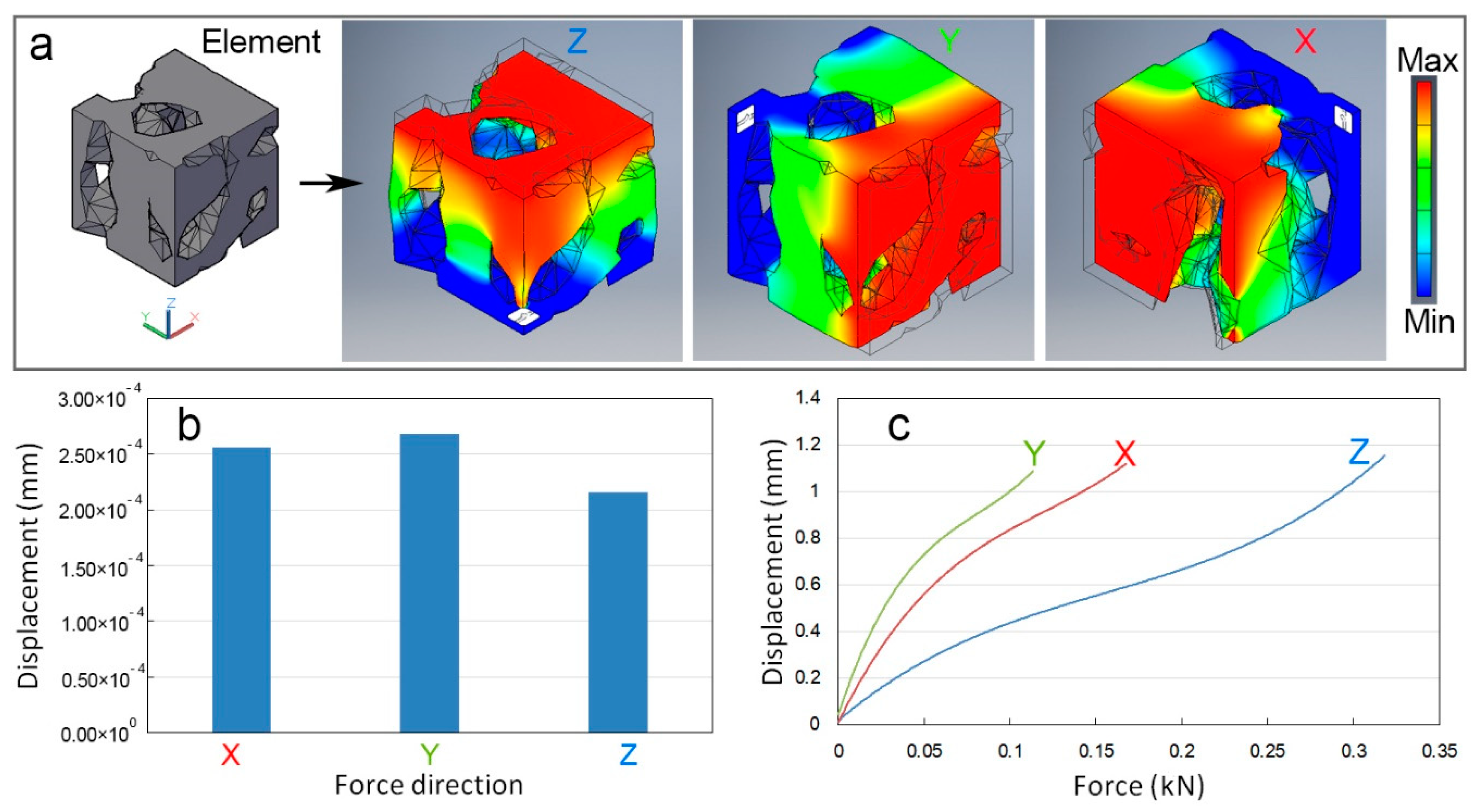
Figure 5.
Composites designed through the permutation of elementary models and compression simulations on composites (using the simulation method descripted in Section 3.3).
Figure 5.
Composites designed through the permutation of elementary models and compression simulations on composites (using the simulation method descripted in Section 3.3).
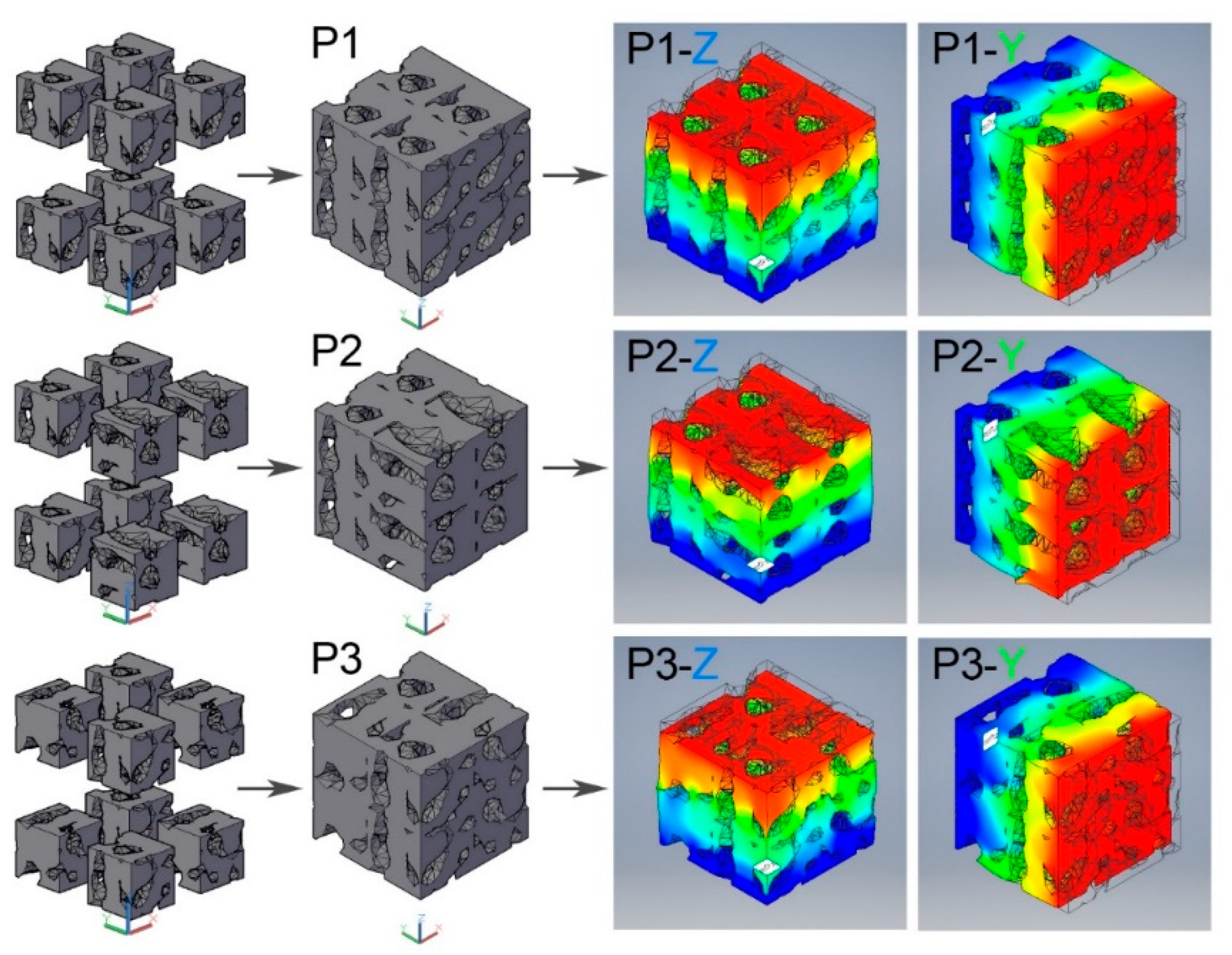
Figure 6.
Displacements along the Z and Y axes under compression with a loading level of 0.5 MPa. (a) The displacement of stressed surface along the Z-axis; (b) The displacement of the stressed surface along the Y-axis. The sums of row/column/layer sum maxima of feature matrices are plotted by the red line.

Figure 7.
Tensor formation methodology for composite models: (a) Elementary model; (b) Feature value of the elementary model in the XY/XZ/YZ planes; (c) Positions of each elementary model in the composite model; (d) Tensor representation of composite models P1, P2, and P3 in feature values.
Figure 7.
Tensor formation methodology for composite models: (a) Elementary model; (b) Feature value of the elementary model in the XY/XZ/YZ planes; (c) Positions of each elementary model in the composite model; (d) Tensor representation of composite models P1, P2, and P3 in feature values.

© 2020 by the authors. Licensee MDPI, Basel, Switzerland. This article is an open access article distributed under the terms and conditions of the Creative Commons Attribution (CC BY) license (http://creativecommons.org/licenses/by/4.0/).
Share and Cite
MDPI and ACS Style
Tao, Y.; Li, Z.; Li, P. A Design and Fabrication Method for Wood-Inspired Composites by Micro X-Ray Computed Tomography and 3D Printing. Appl. Sci. 2020, 10, 1400. https://doi.org/10.3390/app10041400
AMA Style
Tao Y, Li Z, Li P. A Design and Fabrication Method for Wood-Inspired Composites by Micro X-Ray Computed Tomography and 3D Printing. Applied Sciences. 2020; 10(4):1400. https://doi.org/10.3390/app10041400
Chicago/Turabian StyleTao, Yubo, Zelong Li, and Peng Li. 2020. "A Design and Fabrication Method for Wood-Inspired Composites by Micro X-Ray Computed Tomography and 3D Printing" Applied Sciences 10, no. 4: 1400. https://doi.org/10.3390/app10041400
Note that from the first issue of 2016, this journal uses article numbers instead of page numbers. See further details here.