Influence of Vacuum Level on Heat Transfer Characteristics of Maglev Levitation Electromagnet Module


1
Key Laboratory of Traffic Safety on Track, Central South University, Ministry of Education, Changsha 410075, China
2
Joint International Research Laboratory of Key Technologies for Rail Traffic Safety, Changsha 410075, China
3
National and Local Joint Engineering Research Center of Safety Technology for Rail Vehicle, Changsha 410075, China
4
College of Mechanical and Vehicle Engineering, Hunan University, Changsha 410000, China
*
Author to whom correspondence should be addressed.
Appl. Sci. 2020, 10(3), 1106; https://doi.org/10.3390/app10031106
Submission received: 4 January 2020
/
Revised: 29 January 2020
/
Accepted: 4 February 2020
/
Published: 7 February 2020
(This article belongs to the Section Mechanical Engineering)
Abstract
:The vacuum tube transportation (VTT) system has been a promising direction of future transportation. Within this system, a high-speed maglev travels in a low-vacuum environment to reduce aerodynamic drag. However, the heat dissipation of on-board heating devices will be compromised under low-vacuum conditions, and the device performance may thus be lowered. This study investigates the low-vacuum conjugate heat transfer characteristic of a levitation electromagnet module of a maglev using an experimentally verified numerical method. During the heating process, the surface temperature distribution of the levitation electromagnet, and the temperature and velocity characteristics of the flow field are examined. It is found that, as the vacuum level increases from 1.0 atm to 0.1 atm, the total heat dissipating from the levitation electromagnet module is decreased by 49% at 60 min, the contribution of convection heat flux over the total heat flux is decreased from 49% to 17%, and the convection heat transfer coefficient of the levitation electromagnet is decreased by 89%. This study can provide an efficient numerical model for low-vacuum heat transfer study on a VTT system as well as help the evaluation and optimization of low-vacuum maglev thermal management systems.
1. Introduction
Aerodynamic drag is a major source of resistance on operating high-speed trains. For trains operating at a speed of 350 km/h or higher, the aerodynamic drag takes more than 75% of the overall drag [1,2,3]. In order to reduce the aerodynamic drag, the vacuum tube transportation (VTT) system has been proposed. This system adopts a maglev train to eliminate the mechanical friction between rail and wheel. It also creates a low-vacuum environment such that the aerodynamic drag can be greatly reduced [4,5]. Based on the demand for faster and more efficient high-speed railway transportation, various VTT system designs have been proposed [6,7,8]. Despite the huge reduction on aerodynamic resistance, the VTT systems are subjected to a new challenge: under low-vacuum conditions, the convection heat transfer between the heating source of the maglev and the environment will be compromised. This may lead to device overheating and in turn weaken device performances. For example, studies have shown that once the operating temperature of the levitation electromagnet exceeds the designed limit, permanent demagnetization will occur [9,10], and the levitation capacity of the maglev may be sabotaged.
The levitation electromagnet is a key component in a high-speed maglev system. Under operating mode, the input electric current serves for magnetic field generation, while energy loss from Joule heating will also inevitably occur. This Joule heating energy will accumulate within the electromagnet, causing a temperature rise and posing a potential threat on the lifespan of the device and the safety operation of the maglev [11,12]. Compared to trains operating under 1.0 atm, when high-speed trains are operating at a low-vacuum environment, the heat dissipation rate is reduced [13,14] and the maximum temperature of the device will be increased. In this way, the existing cooling design of the levitation electromagnets in the VTT system will be subjected to considerable challenge. Up to now, multiple studies have been conducted to investigate the thermal profile and temperature control solutions of on-board heating devices in maglev, which are based on either an enhanced passive cooling concept [15,16] or an active cooling concept [17].
Low-vacuum heat transfer has been widely investigated in scientific and engineering research [18,19,20]. Typical research approaches include experimental studies and numerical studies. The experimental tests are usually essential in evaluating the thermal properties of novel materials, such as the measurement of thermal conductivity and heat transfer coefficient of nanofilms under vacuum conditions [21]. Numerical studies can conveniently harvest data at any desired location or field and separate the different type of heat flux according to the transport mechanism. For example, the convection heat transfer coefficient [22] as well as the weight of convection and radiation heat transfer over the total of heat flux [23] can be calculated from numerical simulation method. In heat transfer studies related to high-speed trains, Luo et al. [24] and Ji et al. [25] obtained the contribution of convection heat flux and radiation heat flux of on-board heating units through numerical methods and proposed optimization designs. Up to date, the studies regarding cooling performance of on-board heating units on the trains are usually conducted under standard atmosphere pressure. The low-vacuum heat transfer studies for VTT trains are much less reported.
In the numerical methods related to the conjugate heat transfer problem, the key issue is the validity of the numerical model. Therefore, a large amount of conjugate heat transfer studies are based on numerical studies which have been verified by representative experimental tests [26,27,28]. This hybrid method can efficiently generate reliable results at relatively small cost. Hence, considering the model geometry and heat transfer mechanisms involved in this study, a combined numerical and experimental study method is used. There are several numerical approaches which can solve conjugate heat transfer problems. The Lattice Boltzmann Method (LBM) is efficient in dealing with numerical models with complex geometry as well as multiphase flow problems. This approach is widely applied in nanoscale fluid flow or porous media fluid flow problems [29,30]. The Lagrangian meshless methods, such as the Smoothed Particle Hydrodynamics (SPH) method, can handle large-scale deformation of the fluid domain as well as large displacement in solid domains [31]. For the problems regarding conjugate heat transfer in subatmospheric conditions, when the Knudsen number is less than 0.01, the fluid domain can be treated as a continuum medium and the Finite Volume Method (FVM) is a relatively robust approach that has been widely used in numerical studies [32,33]. When the Knudsen number is greater than 0.01, the fluid domain can no longer be treated as a continuum, such that the LBM method can be considered. The maximum Knudsen number appearing in this study has a value less than 0.01; therefore, the FVM method is chosen as the numerical approach in this study.
This study investigates the temperature rise process of a levitation electromagnet module in a maglev under different vacuum levels through an experimentally validated 3-dimensional numerical model. The least-favorable operating condition, which is the static levitation situation of the levitation electromagnet, is comprehensively investigated. Based on existing research conclusions and engineering applicability, the range of the vacuum level is set from 1.0 atm to 0.1 atm. Under the specified vacuum level range, the velocity and temperature distribution of the flow field, as well as the conjugate heat transfer characteristic in the fluid–solid interface, are analyzed. The influence of the flow field on the temperature profile of heating units is studied. By analyzing the convection heat flux and radiation heat flux under different vacuum levels, the low-vacuum heat transfer profile of the levitation electromagnet is characterized. The effective convection heat transfer coefficients under different vacuum levels are then calculated for evaluation of the influence of the vacuum level on the heat transfer characteristics.
2. Numerical Methods
2.1. Physical Model and Boundary Conditions
The geometric model of the levitation electromagnet module is shown in Figure 1a. This structure contains a complete set of levitation electromagnet units on one side of an electromagnet maglev car. The solid model in Figure 1a consists of 12 individual electromagnet units (EMU), which include 6 primary magnet units, 4 core-elevated magnet units and 2 end magnet units. The internal structure of the EMUs is complex. The system is constructed by an electromagnet coil, a steel core, epoxy, and glass fibers. All dimensions are normalized by the height of the EMU (H = 0.12 m). Within the levitation electromagnet module, M1–M6 are the primary magnet units, H1–H4 are the core-elevated magnet units, S1–S2 are the end magnet units. Pm and Pd are the points on the M3 surface, which is located near the gap region of M2 and M3. Based on the objectives of this study, the following assumptions are made to reduce the complexity of the model: (1) The electromagnet coil is considered as one bulk material with homogeneous heating power distribution. (2) The electromagnet coil is assumed to be emitting heat in a constant rate, i.e., the temperature-related heating power change is neglected. (3) For the heat transfer inside of the electromagnet module, since the epoxy functions as a bonding agent between different components, the contact thermal resistance in between the interface of the different solid materials is not considered. The material properties of each component in the levitation electromagnet module are shown in Table 1.
The levitation electromagnet module model in Figure 1a is placed in a 166.67H × 28.33H × 28.33H cuboid space, as illustrated in Figure 1b. The bottom surface of the model is 8.33H above the ground and the geometric center of the model coincides with the geometric center of the cuboid in the horizontal plane (x–y plane in Figure 1b). The initial pressure of the fluid region is assumed to be 0 Pa (gauge pressure) and the initial temperature of both the fluid and solid regions is 295 K, respectively, which is in agreement with the experimental setup. The boundary condition of the closed system is set as non-slip isothermal walls.
2.2. Governing Equations
For fluids under low-vacuum conditions, the validity of fluid dynamic governing equation can be confirmed by the Knudsen number [34]. The definition of Knudsen number is shown in Equation (1),
where and are Knudsen number, Boltzmann constant, fluid temperature, molecular diameter of the fluid, total pressure of fluid and characteristic length of the research object, respectively. In this study, L is the height of the magnet unit (H). Based on the parameters in this study, the maximum Knudsen number calculated from Equation (1) is 1.03 × 10⁻⁴, which is less than the reference threshold of 0.01. Therefore, the air in this study can be treated as a continuum.
For studies on compressible viscous transient flow in natural convection, the continuity equation and the momentum equation can be expressed in the form of Equations (2) and (3), respectively.
where , , , , , and represent the fluid density, reference time frame, velocity vector, surface vector, identity matrix and viscous stress tensor, respectively. is the buoyancy source term defined as , is the reference density and is the gravitational acceleration vector.
This study also involves the energy transfer process and therefore the energy equation needs to be applied to satisfy the conservation of energy requirement. The energy equations for the fluid and solid are shown in Equations (4) and (5), respectively,
where is the density of solid, is the heat flux vector, and are the total energy and enthalpy per unit mass of fluid, and is the specific heat of solid. represents the energy source terms. This energy source term includes the heat source from the coil and the heat flux from radiative heat transfer. The radiation heat flux is obtained by solving the radiative transfer equation, which can be written in the format of Equation (6):
where is the position vector and is the unit vector into a given direction. and are the radiative intensity and black body intensity, respectively. , is the absolute refractive index. For atmospheric and subatmospheric conditions, the refractive index of air is approximately 1. is the Stefan–Boltzmann constant and and are the absorption coefficient and scattering coefficient of the transport medium, respectively. Since air is the transport medium in this study, the value of and are assumed to be zero. is the extinction coefficient defined as . denotes an incoming radiation direction. is the solid angle of . The boundary condition for radiative heat transfer is defined in the format of Equation (7),
where is the wall position vector and is the surface emissivity. In this study, the surface emissivity of all solids is approximated to be 0.8, which is the weighted average of surface emissivity among all components. is the reflectivity and . is the surface normal.
In the numerical model, the heat transfer within both fluid and solid domain obeys Fourier’s law, which is formulated as , where is the conduction heat flux, is the material’s thermal conductivity tensor, and is the spatial temperature gradient.
The conjugate heat transfer method is applied to the fluid–solid interfaces [35]. The energy equation is then solved throughout the solid and fluid domain with implicit thermal coupling. Based on the conjugate heat transfer method, the convection heat transfer coefficient between fluid and solid is not required as the numerical model input. However, the convection heat transfer coefficient is very useful in evaluating the cooling performance of a heated object and can be directly applied to the numerical model when the computational capacity is limited. Therefore, in this study, the convection heat transfer coefficient is derived based on the numerical results according to Equation (8):
where is the convection heat transfer coefficient, is the convection heat flux. and are the surface temperature and reference temperature of the fluid, respectively.
2.3. Numerical Procedure
In the buoyancy-driven natural convection flow, the intensity of flow can be categorized by the Rayleigh number [36,37]. When , the flow is laminar. When , the natural convection flow will transform into a turbulent flow. The definition of number is shown in Equation (9),
where is the local gravitational acceleration and is the characteristic temperature difference, which is set as 100 K in this study. is the thermal expansion coefficient, is the kinematic viscosity, and is the thermal diffusivity of the fluid. According to Equation (9), the calculated maximum Rayleigh number in this study is , which is less than . Therefore, the fluid field follows a laminar flow pattern.
In order to simulate conjugate heat transfer under a subatmospheric environment, the reference pressure of the fluid domain is set in the form of Equation (10). According to the ideal gas law, under a fixed temperature the fluid density is proportional to the pressure. Therefore, the reference density of the air is set to match with the corresponding vacuum level, as shown in Equation (11).
In Equations (10) and (11), is the ratio of environmental pressure to the atmospheric pressure, is the reference pressure, and and are the atmospheric pressure and air density at the atmospheric pressure, respectively.
The commercial code STAR-CCM+ is utilized to carry out the simulations. Both separated-flow and coupled-flow solvers have been used in this study. The results from both solvers exhibit little difference. However, the separated-flow solver requires less computational resources than the coupled-flow solver. Therefore, the separated-flow solver is used. The radiation model adapts DO model. Air is assumed to be the ideal gas. The effect of gravity is also taken into account in the numerical model. In the separated-flow solver, the second-order upwind scheme is adopted for the convection term of the equations. The SIMPLE algorithm is used in the overall solution. The second-order precision is used for time discretization. The time step used in this study is calculated by Equation (12) based on the theoretical study by Adrian [38]:
where is the time constant, is Prandtl Number and is the velocity scale. The minimum value for this study according to Equation (12) is 0.183 s. Based on the results from Equation (12), the iterative time steps of , and have been selected for the convergence test [39]. It is found that when the iterative time step is around 0.18 s, during the heating process, the fluctuation of convection heat transfer coefficient is not negligible. As the time step decreases to a level between 0.04 s and 0.01 s, the numerical stability on the convection heat transfer coefficient can be observed. Hence, the time step of 0.04 s is applied in this study. The stopping criteria for each time step is set as when the residues of continuity equation and velocity equation fall below 10−3 and residues of energy equation fall below 10−6. The vacuum levels investigated in this study include 0.1 atm, 0.3 atm, 0.4atm, 0.5 atm and 1.0 atm.
2.4. Domain Discretization
The numerical model adopts a Cartesian grid system for the discretization of the computational domain through Star-CCM+ software, and some representative schematics of the grid system are shown in Figure 2. An adapted boundary prism layer mesh is used for precise capture of thermal and velocity profiles within the boundary layer [40,41]. For some small-scale geometries in the model, such as the air gap between each EMU, local mesh refinements are applied in order to accurately capture the temperature profile and heat transfer characteristic. Five prism layers with a first-layer thickness of 0.3 mm are generated on the fluid side near the fluid–solid interface to accurately capture the details of fluid flow and heat flux near the interface regions.
In order to check the mesh sensitivity and exploit the efficiency of the numerical method, three sets of mesh are generated with fine, medium and coarse grid levels, respectively.
3. Experimental Validation
3.1. Experimental Setup
The experiment is conducted in a closed adiabatic system. The dimension of the system and the position of the levitation electromagnet module are exactly the same as illustrated in Figure 1. The experimental pressure in the system is maintained at 40 kPa, which corresponds to approximately 0.4 atmosphere pressure. The heating of the electromagnet is controlled by a constant electrical current of 25 A. The resistance of the primary magnet units and core-elevated magnet units is 0.755 Ω while the resistance of the end magnet units is 0.574 Ω. The heating power of each type of magnet unit is shown in Table 1. The heating power of the magnet units is calculated according to Joule’s law: , where is the heating power per unit volume, and are the rated current and internal resistance of the magnet unit, respectively, and is the volume of the coil. This heating power value used in the numerical model and the experimental study is based on the actual operating condition of the EMUs. The initial environmental and device temperature in the experiment is 295 K. The stopping criteria for the experiment is a temperature rise of 100 K in the maximum temperature point of throughout the levitation electromagnet surface. All the temperature measurements are made by T type thermocouples. An uncertainty analysis of temperature measurements was conducted to determine the uncertainty of the measured temperature. The total uncertainty value is given as follows [42]:
where is the fluctuation of measured temperature, is the average temperature of measuring point, and is caused by the accuracy of the T type thermocouples, which is ±0.5 K. is caused by the accuracy of logger readings given by the manufacturer. The maximum contribution of the logger to the errors of T type thermocouples without compensation is ±1.1 K. is caused by measurement error, which is ±0.5 K according to experimental test. According to Equation (13), the combined uncertainty is 1.3%.
3.2. Results Comparison and Analysis
According to all the temperature measurement results obtained from experiment, the point Pm on M3 has been identified as the maximum temperature point on the EMU surface. The 100 K temperature rise of the EMU takes 57 min. In the numerical simulation, the temperature distribution of the magnet surface is also monitored. The maximum temperature region appears near each EMU’s four upper-corner surfaces, which is consistent with the experimental results.
The temperature rises of Pm from both the numerical method and the experimental results are shown in Table 2. The results given by the numerical simulations agree well with the experimental data. At the initial heating process, the temperature from the numerical results rises slightly faster than the experimental results. This is possibly caused by the following reasons: (1) A simplified model of the electromagnet coil system is used in the numerical simulation, while the actual heat source distribution of the coil may not be completely homogeneous and is likely to have a greater temperature near the core area. This actual configuration may result in a lower temperature on the magnet surface. (2) The numerical simulation assumes zero contact thermal resistance so that the heat from the heating coil is conducted to the EMU surface in a faster rate than the experiment. The difference between the experimental data and the numerical results from medium meshes is 2.1%. Considering the accuracy and precision of the numerical calculation and the measurement error in experiments, it can be concluded that the numerical results agree well with the experimental results.
As for the mesh sensitivity study, the medium and fine meshes reflect different levels of refinement on the coarse mesh. The grid numbers of each set of meshes is shown in Table 2. By comparing the temperature rise curve of three sets of mesh to the experimental results, it is found that all mesh levels can match well with the experimental data. The difference between each level of mesh is trivial. Considering that the grid number of the coarse mesh is not sufficient to capture the flow and temperature distribution in the fluid domain, the medium mesh is selected as the discretization scheme of the fluid domain. From the experimental validation and the grid independence test, it can be concluded that the domain discretization parameter and numerical methodology used in this study are sufficient to yield accurate results.
4. Results and Discussion
4.1. Evolution of EMU Surface Temperature Profile during Heating Process
The levitation electromagnet module is heated under five different vacuum levels, where the 1.0 atm heating process can be treated as a reference for evaluating the reduction in heat dissipation and increase of maximum temperature caused by vacuum environment. During the heating process, the maximum temperature rise on each type of EMU is shown in Table 3. For each vacuum level, the EMUs are heated for 60 min. The maximum temperature rise profiles of EMUs exhibit a symmetrical pattern due to the symmetrical distribution of the levitation electromagnet module. In the first 10 min of the heating process, the temperature differences among the 3 types of EMUs are small. After 10 min heating, the temperature rise of the end magnet units appear to be slower than that of the primary magnet units and core-elevated magnet units. This is because the end magnet units are located on both sides of the levitation electromagnet module as illustrated in Figure 1a. The heated air around the end magnet units has more sufficient space for convection heat flow, which in turn lowers the temperature of air near the fluid–solid interface on the end magnet unit and results in a better cooling. Meanwhile, the end magnet units have a lower heat-generation rate than that of the primary magnet units and core-elevated magnet units. This is another reason for the low temperature in the end magnet units. After 20 min of heating, the maximum temperature of the core-elevated magnet units gradually appears to have a slower increase speed than the primary magnet units. This is because the core-elevated magnet unit has an extruded top structure (as shown in Figure 2), which provides more surface area for heat dissipation. Therefore, the primary magnet unit in the levitation electromagnet module is the most likely to have overheating problems among all the EMUs.
In order to further analyze the temperature distribution of the primary magnet units, the maximum temperatures of all the 6 primary magnet units after 60 min of heating are shown in Table 4. According to the results in Table 4, M1 and M6 have the maximum temperature rise, followed by M2 and M5, while M3 and M4 have the lowest temperature rises among all the heating magnet units. It should be noted that in the experimental section, it is mentioned that the maximum-temperature point appears at point Pm on M3. However in the simulation analysis it is found that the maximum temperature among EMUs appears at M1 and M6. This is because the thermocouple in the experiment was not placed at an exact position with the maximum temperature in M1 and M6. However, the vertical height of point Pm does agree with the height of the maximum-temperature points in M1 and M6. In order to explain the temperature difference between EMUs, local temperature and velocity contours in the gap region of EMUs are shown in Figure 3. According to the velocity contour in Figure 3a,b, the heated air is driven by buoyancy force and flow towards the upper part of the fluid domain. This buoyancy flow therefore creates a low-pressure region on the lower part of the levitation electromagnet, and the low-pressure region is then filled by the unheated air on the bottom part of the fluid domain. This phenomenon explains the cause of spatial variance of temperature in the fluid domain. Additionally, it can be observed from Figure 3a that a local flow separation between H2 and M1 is formed. The flow velocity is decreased due to the increase in cross section near the flow separation region depicted in Figure 3a, the convection heat flow on the side of M1 is then compromised and therefore leads to a higher temperature of the M1 unit. The phenomenon shown in Figure 3a,c can also be observed between M6 and H3. As for the air-gap region between M3 and M4, the buoyance-driven flow has a higher speed than the region between H2 and M1, which in turn leads to a lower fluid temperature and better cooling performance. This explains the variance of maximum temperature among EMUs as shown in Table 4. Based on the analysis above, the M6 unit is selected for the proceeding quantitative analysis on thermal characteristics of EMUs.
The heat dissipation of the levitation electromagnet is influenced by the convection heat flux and radiation heat flux on the solid–fluid interface. These factors contributed to three different temperature profiles on the surface of each EMU during the heating process. Figure 4 shows the surface temperature distribution of M6 during the heating process at some representative time frames and vacuum levels. The three reference time frames are selected as t1, t2 and t3, where t1= 3 min, t2=10 min and t3= 60 min.
At the initial heating process t1, the heating of the EMU is relatively homogeneous. Only small a temperature rise can be observed on the unit surface except for the regions near the EMU’s heating coil. Between time t1 and t2, under the influence of buoyancy flow, the upper part of each EMU is subjected to higher environmental temperature, therefore leading to the concentration of a high-temperature area around the unit’s upper surface. During this time period, the maximum temperature rise appears on the side surface in the junctions of two adjacent units. On the top surface of the magnet, as the heat flux conducts from the coil to the core structure, concentric thermal contours are formed.
After 60 min of heating, a relatively steady thermal state has been reached on the EMU surface. The temperature gradient in the fluid domain becomes greater during the heating process due to inadequate convection heat transfer. As a result, the accumulated heat in the EMU leads to a further concentration of a high-temperature region and higher temperature variance around the EMU surface. Among the unit’s surface, the maximum temperature rise appears near the magnet coil’s four upper corners, which agrees with the experimental result. The temperature distribution profile on the surface of the EMU is influenced by the unit’s adjacent unit structure, where the neighboring unit types of M6 are the primary magnet unit and the core-elevated magnet unit, according to Figure 1. The different type of neighboring EMU will result in different thermal contours on the side of M6.
4.2. Influence of Vacuum Level on Temperature Distribution of EMU Surface and Fluid Field
Based on the results in the reference case (1.0 atm), under standard atmosphere pressure, the convection heat transfer flux takes 49% of the total heat flux at 60 min. At a low-vacuum environment, the convection heat transfer will be compromised with the decrease of air density. Therefore, it is important to investigate the influence of vacuum level on the EMU temperature rise. The influence of vacuum level on temperature distribution of M6 can be compared in each row of Figure 4, in that each row in Figure 4 represents the surface temperature profile of M6 under different vacuum levels at the same reference time frame of the heating process. According to the comparison results, it is found that the maximum temperature in the EMU becomes higher along with the decrease of environmental pressure as a result of weakened convection heat transfer. After 3 min of heating, the magnet surface under 0.1 atm and 0.3 atm has a higher maximum temperature gradient than that under 1.0 atm. This difference in temperature gradient under different vacuum levels becomes more obvious over time. After 10 min of heating, a high-temperature region can be observed on the side of the magnet unit for 0.1 atm and 0.3 atm heating cases. However, this high-temperature region is not very obvious for the magnet unit heating under 1.0 atm. The temperature of air around the EMU surface is also increased in low-pressure cases due to the elevated temperature of the EMU surface.
The influence of vacuum level on the convection heat transfer is also reflected on the flow field around the levitation electromagnet. Figure 5 shows the flow velocity distribution on the symmetric plane of the fluid domain that is perpendicular to the y direction according to Figure 1b. The EMUs in Figure 5 are heated for 60 min at two different vacuum levels. It can be observed that during the heating process, the buoyancy force drives the heat flow upwards, and the low-pressure region created by the heat flow is filled by the unheated air. In this way, some mid-scale circulation flow can be observed in the fluid domain.
Compared with the flow field under 0.1 atm, the fluid convection under 1.0 atm has a larger impact area. Meanwhile, the velocity vector above the levitation electromagnet has a relatively uniform upward alignment direction. This is because the buoyancy flow becomes the dominant flow type and its intensity is proportional to the air density. With the increment of environmental pressure, the flow velocity on both sides of the levitation electromagnet also increases. Except for the surfaces that are located on both side of the air gaps between different EMUs, the rest of the side surfaces on the EMU gets a higher convection-induced cooling heat flux under a 1.0 atm case due to the more-adequate convection in the fluid domain. For the flow field above the top levitation electromagnet module, the flow velocity near the gap region is greater than the flow velocity above the EMUs’ top surface. This is because the core of each EMU is not a power source and therefore has a relatively low temperature, which in turn results in a much weaker buoyancy force than the air-gap region. This phenomenon gets more significant as the environmental pressure increases.
The effect of natural convection on temperature distribution of the flow field around the levitation electromagnet is then analyzed. Figure 6 shows the temperature and temperature gradient along the surface’s outer-normal direction of measuring point Pd. The horizontal axis represents the location at different distances away from the measurement points along the surface’s outer-normal direction (referred in Figure 6 as Y distance). It is shown that under low-pressure conditions, the space variance of the temperature gradient magnitude becomes smaller. In low-pressure cases, the temperature gradient along the surface normal direction tends to decrease in a linear trend.
For all cases investigated in this study, the maximum temperature gradient appears near the fluid–solid interface region. The maximum absolute value of temperature gradient under 0.1 atm is 0.59 K/mm. Compared with the maximum temperature gradient under 1.0 atm, which is 2.55 K/mm, the lowered environmental pressure has led to a 77% decrease of the absolute value of the temperature gradient. This indicates that the lowered pressure has also caused the decrease of convection buoyancy flow in the flow field, which further worsened the heat dissipation of the levitation electromagnet module.
The low-vacuum environment has resulted in reduced convection heat flux and therefore leads to a faster heating process of the levitation electromagnet module. Figure 7 gives the temperature rise curve of the maximum temperature point on the EMU surface during the heating process under different vacuum levels. As the environmental pressure decreases, the time–temperature curve exhibits a higher increase rate. The 100 K temperature rise process under 0.1 atm takes approximately 51 min, which is 23% faster compared to the temperature rise time at 1.0 atm. The summarized temperature rise time under different vacuum levels is shown in Table 5. According to Table 5, it can be concluded that, if the existing levitation electromagnet module is operating without additional cooling devices or methods, the operation time of the vacuum maglev should be limited to avoid device overheating.
4.3. Influence of Vacuum Level on Heat Transfer Characteristics
It has been shown that the low-vacuum environment can significantly reduce the convection heat flux. Therefore, quantitative analysis of the vacuum level influence on convection heat transfer capacity is carried out. Figure 8 shows the averaged surface convection heat flux of the EMU during the heating process under different vacuum levels. The difference in convection heat flux magnitude gets bigger along the heating process. At the end of the heating process, the average surface convection heat flux of 1.0 atm and 0.1 atm are 644 W/m2 and 104 W/m2, respectively, which indicates that the low-vacuum condition can cause an 84% reduction in heat flux.
As the vacuum level increases, the dominant heat dissipation approach under vacuum condition will transfer from convection heat transfer to radiation heat transfer. Figure 9 gives the quantitative description of the weight of convection heat transfer flux over the total heat transfer flux (Φ) under different vacuum levels. Under 1.0 atm, the convection heat flux takes 49% of the overall heat flux at 60 min. While under 0.1 atm, the convection heat transfer flux takes only 17% of the overall heat transfer flux. At each vacuum level, the percentage of convection heat flux firstly increases and then decreases along the heating process. This is because during the initial stage of magnet heating, the surface temperature rise is insignificant. According to the Stefan–Boltzmann law, the radiation heat flux is proportional to the 4th power of the temperature difference between the solid–fluid interface. In contrast, the convection heat flux is linearly proportional to this temperature difference. Therefore, during the heating process, when the temperature difference is small, the increase in radiation heat flux is insignificant. In contrast, the convection heat flux is more sensitive to the small temperature difference in the beginning stage. Thus, the curve in Figure 9 shows an increasing trend during the initial heating stage. As the temperature difference gradually builds up, the radiation heat flux increases significantly faster than the convection heat flux. This explains the decrease of Φ in Figure 9. It can be seen from Figure 9 that due to the higher temperature rise rate of the levitation electromagnets in a low-pressure condition, the inflection points on the curve are also advanced in the x axis, which indicates that the low-vacuum condition facilitates the transition of convection heat flux to radiation heat flux. The appearing time of inflection point is shown in Table 6. It can be concluded that the low-vacuum environment evidently lowered the convection heat flux of the levitation electromagnets. On the other hand, the temperature rise enhances the radiation heat flux of the levitation electromagnets.
The total heat flux is significantly reduced along with the pressure drop. Among all investigated scenarios, the proportions of convection heat flux at each vacuum level are all less than 50%. At 1.0 atm, the convection heat transfer and radiation heat transfer each takes approximately 50% of the overall heat flux. As the environmental pressure gets smaller, the radiation heat transfer becomes the dominant heat transfer approach. Under 0.1 atm, although the magnitude of radiation heat flux decreases compared with higher pressure cases, the weight of radiation heat flux over the total heat flux increases significantly. The radiation heat flux takes more than 80% of the overall heat flux under 0.1 atm. Based on the results in this study, at low-vacuum conditions, the radiation heat flux serves as the dominant heat transfer approach. As the environmental pressure gets lower, the difference between convection heat flux and radiation heat flux gradually increases. Figure 10 shows the influence of vacuum level on accumulated total and convection heat through the magnet surface over different vacuum levels under selected time frame. As the vacuum level increases from 1.0 atm to 0.1 atm, the total heat dissipating from levitation electromagnet is decreased by 49% (with more than 80% reduction of convection heat). A regression analysis is conducted to better capture the trend. It is found that both the total heat and convection heat can be well represented by a quadratic equation which contains the vacuum level term. In Figure 10a, the fitted curve has an R2 value greater than 0.999, while the fitted curve has an R2 value greater than 0.996 in Figure 10b. Therefore, it can be concluded that the total heat and the convection heat are approximately proportional to the square of the vacuum level.
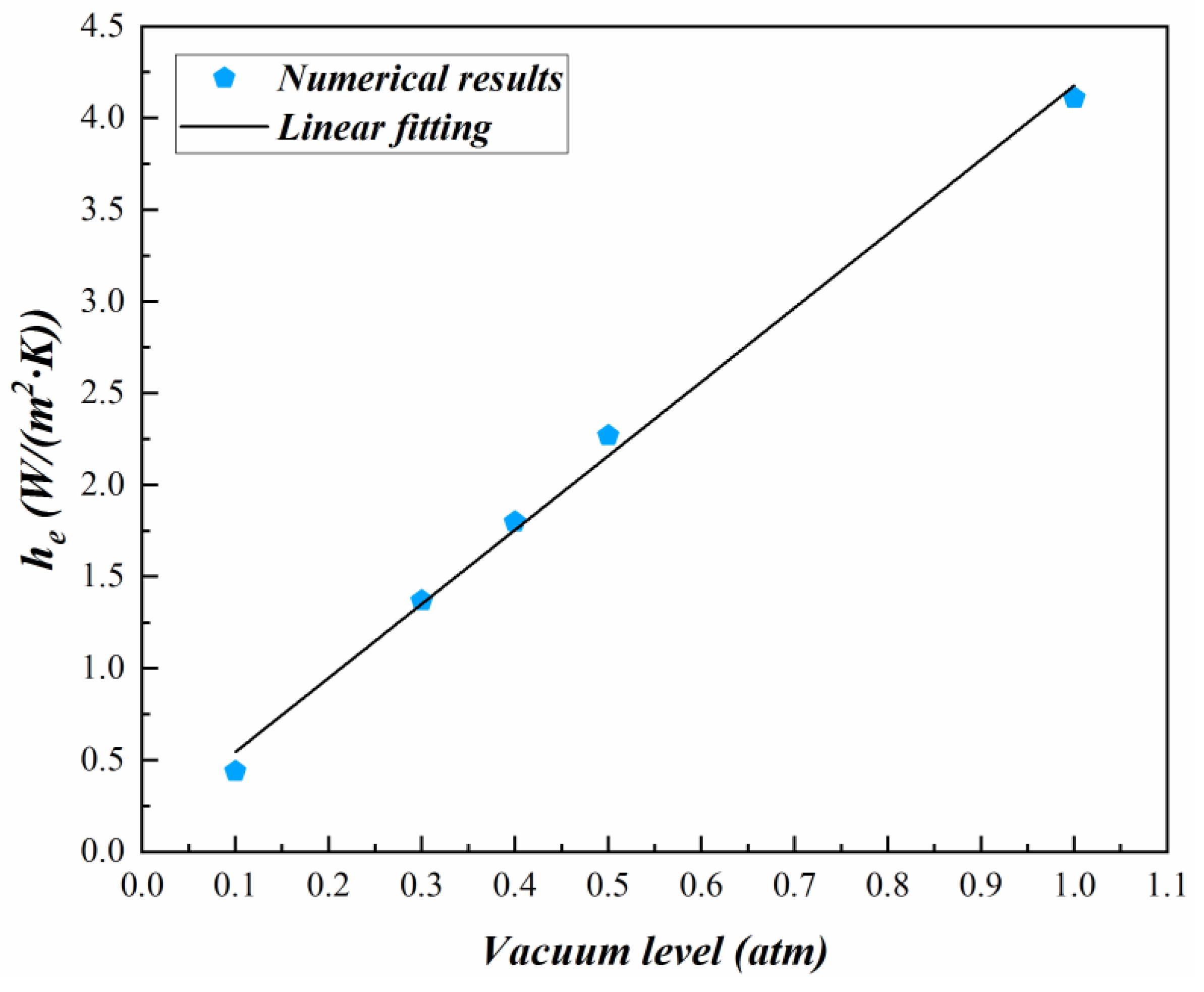
The convection heat transfer coefficient reflects the magnitude of convection heat transfer through the solid–fluid interface. This coefficient is a simplification and approximation of rigorous mathematical derivation. In numerical study and industrial research on conjugate heat transfer problems, the application of convection heat flux can effectively reduce the computation time and cost. The convection heat transfer coefficient can be affected by many factors such as external flow type (laminar flow and turbulent flow) and temperature of the solid surface. Both factors make it very challenging to predict [43]. Experiments usually measure convection heat transfer coefficients based on calibrated samples under typical conditions. The derived convection heat transfer coefficients are then applied to the entire system subsequent research [44]. In this study, the effective convection heat transfer coefficient is derived based on the numerical results according to Equation (8). The results show that during the heating process, under each vacuum level, the convection heat transfer coefficient has a variance of less than 10%. Therefore, a weighted average value of convection heat transfer coefficient is taken, this averaged convection heat transfer coefficient is referred as effective heat transfer coefficient (he). This effective convection heat transfer coefficient decreases with lowered environment pressure. Table 7 shows the effective convection heat transfer coefficient of the EMU under different vacuum levels. Figure 11 shows the regression analysis on effective convection heat transfer coefficient and the vacuum level. The results from regression analysis indicate that the effective convection heat transfer coefficient of EMUs is linearly proportional to the vacuum level. When the vacuum is reduced to 0.1 atm, the effective convection heat transfer coefficient is less than 0.5 W/(m2∙K).
5. Conclusions
This study analyzed the low-vacuum heat dissipation process of a levitation electromagnet module in a maglev train. An experimentally verified numerical model has been established. A complete levitation electromagnet module, which contains 12 individual units, is used for thermal profile characterization. The numerical study on static heating of the levitation electromagnet is carried out under vacuum levels ranging from 0.1 atm to 1.0 atm. The flow field, temperature field of the fluid domain, the temperature distribution profile on the levitation electromagnet surface and heat transfer parameters during the heating process are characterized and analyzed.
Throughout this study, the high-temperature region in the levitation electromagnet module surface has been identified. During the heating process, the high-temperature area is located around four upper corners of each electromagnet unit in the levitation electromagnet module. With the reduction of environmental pressure, the temperature rise rate at the solid–fluid interface is significantly increased. Compared to 1.0 atm, the 100 K temperature rise process under 0.1 atm is shortened by 15.5 min, which indicates a 23% decrease in heating time. Meanwhile, it is found that at 1.0 atm, the radiation heat flux and convection heat flux from the heated levitation electromagnets are approximately equal. With the decrease of environmental pressure, the radiation heat transfer gradually becomes the dominant cooling heat flux. Under 0.1 atm, the radiation heat transfer takes more than 80% of the total heat flux. Meanwhile, this study derived the effective convection heat transfer coefficient under low-vacuum conditions. It is found that under the vacuum levels used in this study, the effective convection heat transfer coefficient varies between 0.4 W/(m2∙K) and 4.1 W/(m2∙K). A regression analysis is conducted between the effective convection heat transfer coefficient and vacuum level. As a result, a linear relationship between these two factors is established.
This study has pioneered the research on a maglev train cooling system capacity under low-vacuum conditions. The outcome of this research could serve as an important reference for the design of maglev trains in a VTT system. The temperature and heat transfer coefficient profile of the levitation electromagnet can help with the understanding on the influence of vacuum level on a maglev cooling system. Moreover, the high-temperature area on the levitation electromagnet module surface can guide the design and optimization of the maglev cooling system. The experimentally verified numerical method established in this study can serve as an efficient tool for analyzing the heat transfer of maglev trains under low-vacuum conditions.
Author Contributions
Y.M. has executed the study, collected and analyzed data, wrote and revised the paper; T.W. and F.W. have provided guidance on numerical simulation; M.Y. has acquired the funding, review and validated the methodology, B.Q. has conceived, designed, and executed the study project, wrote, reviewed and finalized the manuscript; All authors have read and agreed to the published version of the manuscript.
Funding
This research was supported by the National Key R&D Program of China (Grant number: 2016YFB1200602-11), the Strategic Consultation Program from Chinese Academy of Engineering (Grant number: 2018-ZD-16), and the Graduate Student Independent Innovation Project of Central South University (Grant Number: 2019zzts548).
Acknowledgments
The authors acknowledge the computing resources provided by the High-Speed Train Research Centre of Central South University, China.
Conflicts of Interest
The authors declare no conflict of interest.
References
- Tian, H.Q. Formation mechanism of aerodynamic drag of high-Speed train and some reduction measures. J. Cent. South Univ. Technol. 2009, 1, 166–171. [Google Scholar] [CrossRef]
- Zhang, L.; Yang, M.-Z.; Liang, X.-F. Experimental study on the effect of wind angles on pressure distribution of train streamlined zone and train aerodynamic forces. J. Wind Eng. Ind. Aerodyn. 2018, 174, 330–343. [Google Scholar] [CrossRef]
- Wang, T.; Wu, F.; Yang, M.; Ji, P.; Qian, B. Reduction of pressure transients of high-Speed train passing through a tunnel by cross-section increase. J. Wind Eng. Ind. Aerodyn. 2018, 183, 235–242. [Google Scholar] [CrossRef]
- Kim, T.-K.; Kim, K.-H.; Kwon, H.-B. Aerodynamic characteristics of a tube train. J. Wind Eng. Ind. Aerodyn. 2011, 99, 1187–1196. [Google Scholar] [CrossRef]
- Ma, J.; Zhou, D.; Zhao, L.; Zhang, Y.; Zhao, Y. The approach to calculate the aerodynamic drag of maglev train in the evacuated tube. J. Mod. Transp. 2013, 21, 200–208. [Google Scholar] [CrossRef] [Green Version]
- Jia, W.; Wang, K.; Cheng, A.; Kong, X.; Cao, X.; Li, Q. Air flow and differential pressure characteristics in the vacuum tube transportation system based on pressure recycle ducts. Vacuum 2018, 150, 58–68. [Google Scholar] [CrossRef]
- Deng, Z.; Zhang, W.; Zheng, J.; Ren, Y.; Jiang, D.; Zheng, X.; Zhang, J.; Gao, P.; Lin, Q.; Song, B.; et al. A High-Temperature Superconducting Maglev Ring Test Line Developed in Chengdu, China. IEEE Trans. Appl. Supercond. 2016, 26, 1–8. [Google Scholar] [CrossRef]
- Lee, H.W.; Park, C.B.; Lee, J. Improvement of thrust force properties of linear synchronous motor for an ultra-High-Speed tube train. IEEE Trans. Magn. 2011, 47, 4629–4634. [Google Scholar] [CrossRef]
- Bergqvist, A.; Lin, D.; Zhou, P. Temperature-Dependent vector hysteresis model for permanent magnets. IEEE Trans. Magn. 2014, 50, 345–348. [Google Scholar] [CrossRef]
- Zhou, P.; Lin, D.; Xiao, Y.; Lambert, N.; Rahman, M.A. Temperature-Dependent demagnetization model of permanent magnets for finite element analysis. IEEE Trans. Magn. 2012, 48, 1031–1034. [Google Scholar] [CrossRef]
- Huang, Z.; Deng, Z.; Jin, L.; Hong, Y.; Zheng, J.; Rodriguez, E.F. Numerical simulation and experimental analysis on the AC Losses of HTS bulks levitating under a varying external magnetic field. IEEE Trans. Appl. Supercond. 2019, 29, 1–5. [Google Scholar] [CrossRef]
- Del-Valle, N.; Sanchez, A.; Navau, C.; Chen, D.X. A theoretical study of the influence of superconductor and magnet dimensions on the levitation force and stability of maglev systems. Supercond. Sci. Technol. 2008, 21, 125008. [Google Scholar] [CrossRef]
- Niu, J.; Sui, Y.; Yu, Q.; Cao, X.; Yuan, Y. Numerical study on the impact of Mach number on the coupling effect of aerodynamic heating and aerodynamic pressure caused by a tube train. J. Wind Eng. Ind. Aerodyn. 2019, 190, 100–111. [Google Scholar] [CrossRef]
- Zhou, P.; Zhang, J.; Li, T.; Zhang, W. Numerical study on wave phenomena produced by the super high-Speed evacuated tube maglev train. J. Wind Eng. Ind. Aerodyn. 2019, 190, 61–70. [Google Scholar] [CrossRef]
- Vermilyea, M.E.; Minas, C. A cryogen-Free superconducting magnet design for maglev vehicle applications. IEEE Trans. Appl. Supercond. 1993, 444–447. [Google Scholar] [CrossRef]
- Mizuno, K.; Ogata, M.; Hasegawa, H. Manufacturing of a REBCO racetrack coil using thermoplastic resin aiming at Maglev application. Phys. C Supercond. Its Appl. 2015, 518, 101–105. [Google Scholar] [CrossRef]
- Chung, Y.D.; Kim, D.W.; Lee, C.Y. Transfer Efficiency and Cooling Cost by Thermal Loss based on Nitrogen Evaporation Method for Superconducting MAGLEV System. J. Phys. Conf. Ser. 2017, 871, 012095. [Google Scholar] [CrossRef] [Green Version]
- Rahimi, A.; Dehghan Saee, A.; Kasaeipoor, A.; Hasani Malekshah, E. A comprehensive review on natural convection flow and heat transfer: The most practical geometries for engineering applications. Int. J. Numer. Methods Heat Fluid Flow. 2019, 29, 834–877. [Google Scholar] [CrossRef]
- Ross-Jones, J.; Gaedtke, M.; Sonnick, S.; Rädle, M.; Nirschl, H.; Krause, M.J. Conjugate heat transfer through nano scale porous media to optimize vacuum insulation panels with lattice Boltzmann methods. Comput. Math. Appl. 2019, 77, 209–221. [Google Scholar] [CrossRef]
- Garceau, N.; Bao, S.; Guo, W. Heat and mass transfer during a sudden loss of vacuum in a liquid helium cooled tube-Part I: Interpretation of experimental observations. Int. J. Heat Mass Transf. 2019, 129, 1144–1150. [Google Scholar] [CrossRef]
- Zhang, X.; Xie, H.; Fujii, M.; Takahashi, K.; Ikuta, T.; Ago, H.; Abe, H.; Shimizu, T. Experimental study on thermal characteristics of suspended platinum nanofilm sensors. Int. J. Heat Mass Transf. 2006, 49, 3879–3883. [Google Scholar] [CrossRef]
- Zanino, R.; Richard, L.S.; Subba, F.; Corpino, S.; Izquierdo, J.; Le Barbier, R.; Utin, Y. CFD analysis of a regular sector of the ITER vacuum vessel. Part II: Thermal-Hydraulic effects of the nuclear heat load. Fusion Eng. Des. 2013, 88, 3248–3262. [Google Scholar] [CrossRef] [Green Version]
- De Beer, M.; Du Toit, C.G.; Rousseau, P.G. A methodology to investigate the contribution of conduction and radiation heat transfer to the effective thermal conductivity of packed graphite pebble beds, including the wall effect. Nucl. Eng. Des. 2017, 314, 67–81. [Google Scholar] [CrossRef]
- Luo, Z.; Zuo, J. Conjugate heat transfer study on a ventilated disc of high-Speed trains during braking. J. Mech. Sci. Technol. 2014, 28, 1887–1897. [Google Scholar] [CrossRef]
- Ji, P.; Wu, F.; Zhang, G.; Yin, X.; Vainchtein, D. A novel numerical approach for investigation of the heat transport in a full 3D brake system of high-speed trains. Numer. Heat Transf. Part A Appl. 2019, 75, 824–840. [Google Scholar] [CrossRef]
- Maakala, V.; Järvinen, M.; Vuorinen, V. Computational fluid dynamics modeling and experimental validation of heat transfer and fluid flow in the recovery boiler superheater region. Appl. Therm. Eng. 2018, 139, 222–238. [Google Scholar] [CrossRef]
- Baudoin, A.; Saury, D.; Boström, C. Optimized distribution of a large number of power electronics components cooled by conjugate turbulent natural convection. Appl. Therm. Eng. 2017, 124, 975–985. [Google Scholar] [CrossRef]
- Tao, Y.; Yang, M.; Qian, B.; Wu, F.; Wang, T. Numerical and Experimental Study on Ventilation Panel Models in a Subway Passenger Compartment. Engineering 2019, 5, 329–336. [Google Scholar] [CrossRef]
- He, Y.L.; Liu, Q.; Li, Q.; Tao, W.Q. Lattice Boltzmann methods for single-Phase and solid-Liquid phase-Change heat transfer in porous media: A review. Int. J. Heat Mass Transf. 2019, 129, 160–197. [Google Scholar] [CrossRef] [Green Version]
- Goodarzi, M.; D’Orazio, A.; Keshavarzi, A.; Mousavi, S.; Karimipour, A. Develop the nano scale method of lattice Boltzmann to predict the fluid flow and heat transfer of air in the inclined lid driven cavity with a large heat source inside, Two case studies: Pure natural convection & mixed convection. Phys. A Stat. Mech. Its Appl. 2018, 509, 210–233. [Google Scholar] [CrossRef]
- Shadloo, M.S.; Oger, G.; Le Touzé, D. Smoothed particle hydrodynamics method for fluid flows, towards industrial applications: Motivations, Current state, And challenges. Comput. Fluids 2016, 136, 11–34. [Google Scholar] [CrossRef]
- Fu, Z.; Yu, X.; Shang, H.; Wang, Z.; Zhang, Z. A new modelling method for superalloy heating in resistance furnace using FLUENT. Int. J. Heat Mass Transf. 2019, 128, 679–687. [Google Scholar] [CrossRef]
- Oh, Y.W.; Choi, Y.S.; Ha, M.Y.; Min, J.K. A numerical study on the buoyancy effect around slanted-pin fins mounted on a vertical plate (Part-I: Laminar natural convection). Int. J. Heat Mass Transf. 2019, 132, 731–744. [Google Scholar] [CrossRef]
- Tsien, H.S. Superaerodynamics, Mechanics of Rarefied Gases. In Collected Works of Hsue-Shen Tsien (1938–1956); Shanghai Jiao Tong University Press: Shanghai, China; Academic Press: Oxford, UK, 2012; ISBN 9780123982773. [Google Scholar]
- Dorfman, A.S. Conjugate Problems in Convective Heat Transfer; CRC Press: Boca Raton, FL, USA, 2009; ISBN 9781420082388. [Google Scholar]
- Pilkington, A.; Rosic, B.; Tanimoto, K.; Horie, S. Prediction of natural convection heat transfer in gas turbines. Int. J. Heat Mass Transf. 2019, 141, 233–244. [Google Scholar] [CrossRef]
- Nakao, K.; Hattori, Y.; Suto, H. Numerical investigation of a spatially developing turbulent natural convection boundary layer along a vertical heated plate. Int. J. Heat Fluid Flow 2017, 63, 128–138. [Google Scholar] [CrossRef]
- Adrian, B. Convection Heat Transfer, 1st ed.; John Wiley & Sons: New York, NY, USA, 2016; pp. 53–101. ISBN 9781493925650. [Google Scholar]
- Janssen, R.J.A.; Henkes, R.A.W.M. Accuracy of finite–Volume discretizations for the bifurcating natural–Convection flow in a square cavity. Numer. Heat Transf. Part B Fundam. 1993, 24, 194–207. [Google Scholar] [CrossRef]
- Maystrenko, A.; Resagk, C.; Thess, A. Structure of the thermal boundary layer for turbulent Rayleigh-Bénard convection of air in a long rectangular enclosure. Phys. Rev. E-Stat. Nonlinear Soft Matter Phys. 2007, 75, 066303. [Google Scholar] [CrossRef] [PubMed] [Green Version]
- Talbot, L.; Cheng, R.K.; Schefer, R.W.; Willis, D.R. Thermophoresis of particles in a heated boundary layer. J. Fluid Mech. 1980, 101, 737–758. [Google Scholar] [CrossRef] [Green Version]
- Kline, S.J. The purposes of uncertainty analysis. J. Fluids Eng. Trans. ASME 1985, 107, 153–160. [Google Scholar] [CrossRef]
- ISO 8990 ISO 8990 Thermal insulation—Determination of steady-State thermal transmission properties—Calibrated and guarded hot box. BSI 1994. [CrossRef]
- Fang, Y.; Eames, P.C.; Norton, B.; Hyde, T.J. Experimental validation of a numerical model for heat transfer in vacuum glazing. Sol. Energy 2006, 80, 564–577. [Google Scholar] [CrossRef]
Figure 1.
Schematic of model geometry. (a) Levitation electromagnet module and locations of measuring points; (b) Schematic of computational domain, where the enclosed white area represents fluid domain and the shadowed area represents the levitation electromagnet module.
Figure 1.
Schematic of model geometry. (a) Levitation electromagnet module and locations of measuring points; (b) Schematic of computational domain, where the enclosed white area represents fluid domain and the shadowed area represents the levitation electromagnet module.
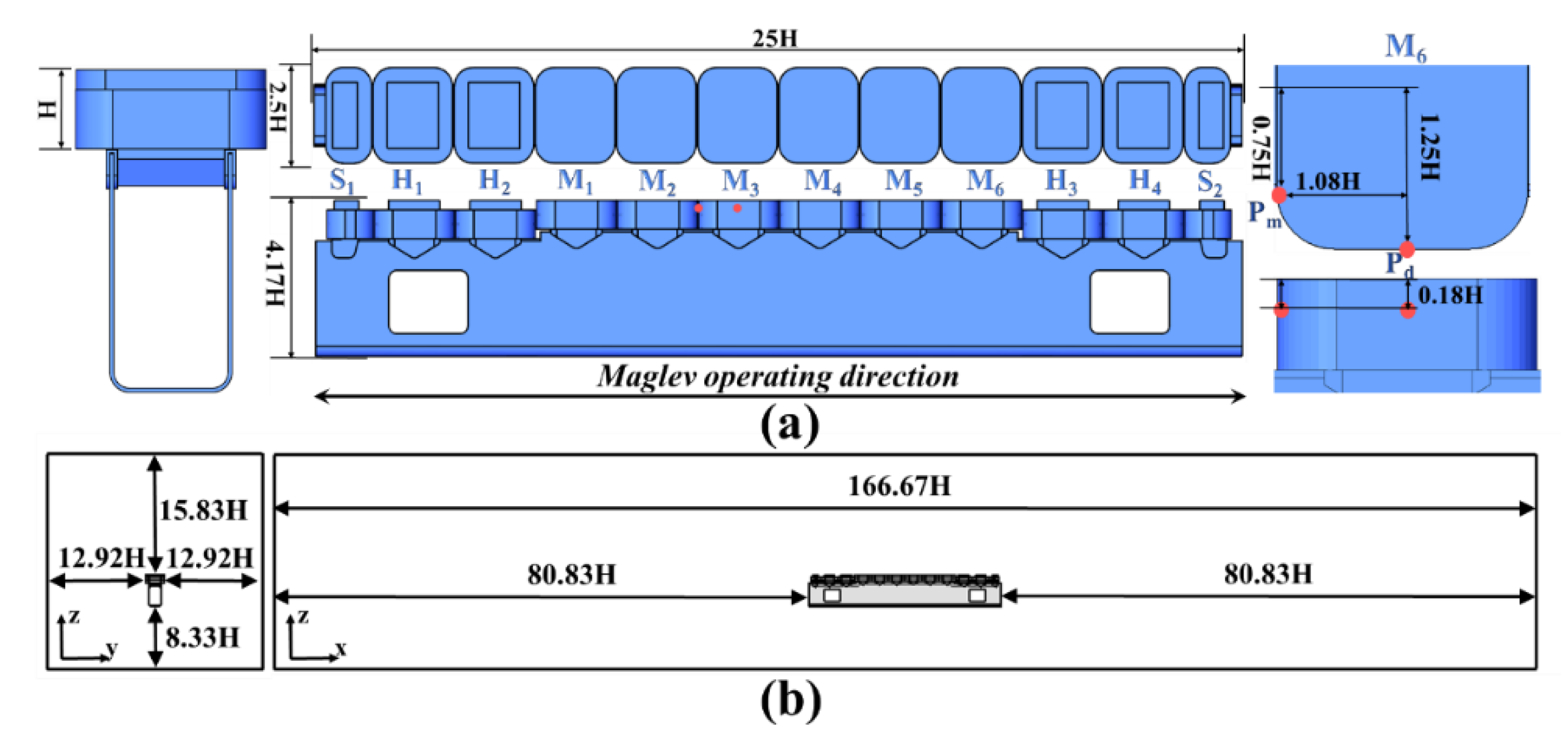
Figure 2.
Discretization of computational model: (a) Overview of the levitation electromagnet region mesh on the symmetric plane; (b) Detailed mesh view of primary magnet unit; (c) Surface mesh of end magnet unit and core-elevated magnet unit.
Figure 2.
Discretization of computational model: (a) Overview of the levitation electromagnet region mesh on the symmetric plane; (b) Detailed mesh view of primary magnet unit; (c) Surface mesh of end magnet unit and core-elevated magnet unit.
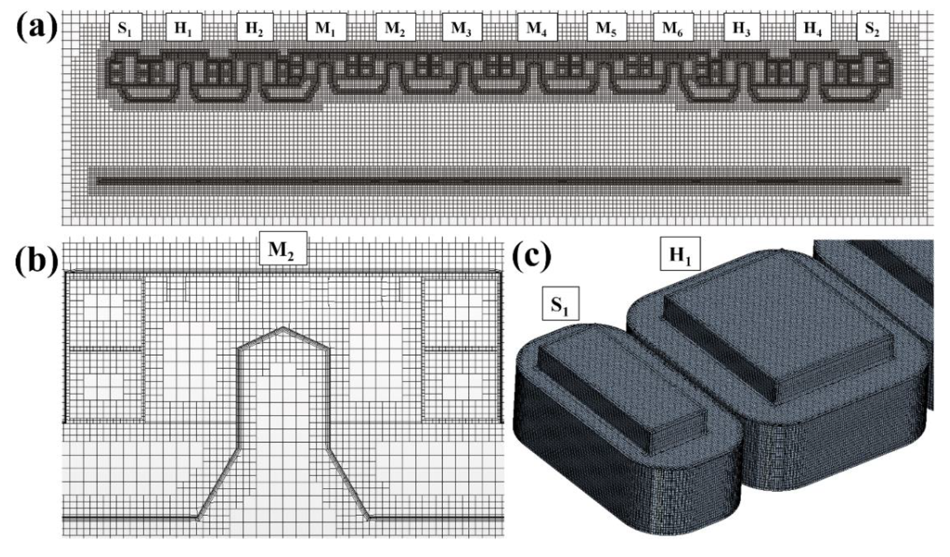
Figure 3.
Local contour near the maximum temperature point of primary magnet units after 60 min of heating under 1.0 atm. This contour cross section is parallel to xz plane in Figure 1 and is 0.75 H away from the symmetric plane of the levitation electromagnet module in y direction. (a) Velocity contour near the maximum temperature point between H2 and M1, where the arrows represent velocity vector; (b) Velocity contour near the maximum temperature point between M3 and M4, where the arrows represent velocity vector; (c) Temperature contour near the maximum temperature point between H2 and M1; (d) Temperature contour near the maximum temperature point between M3 and M4.
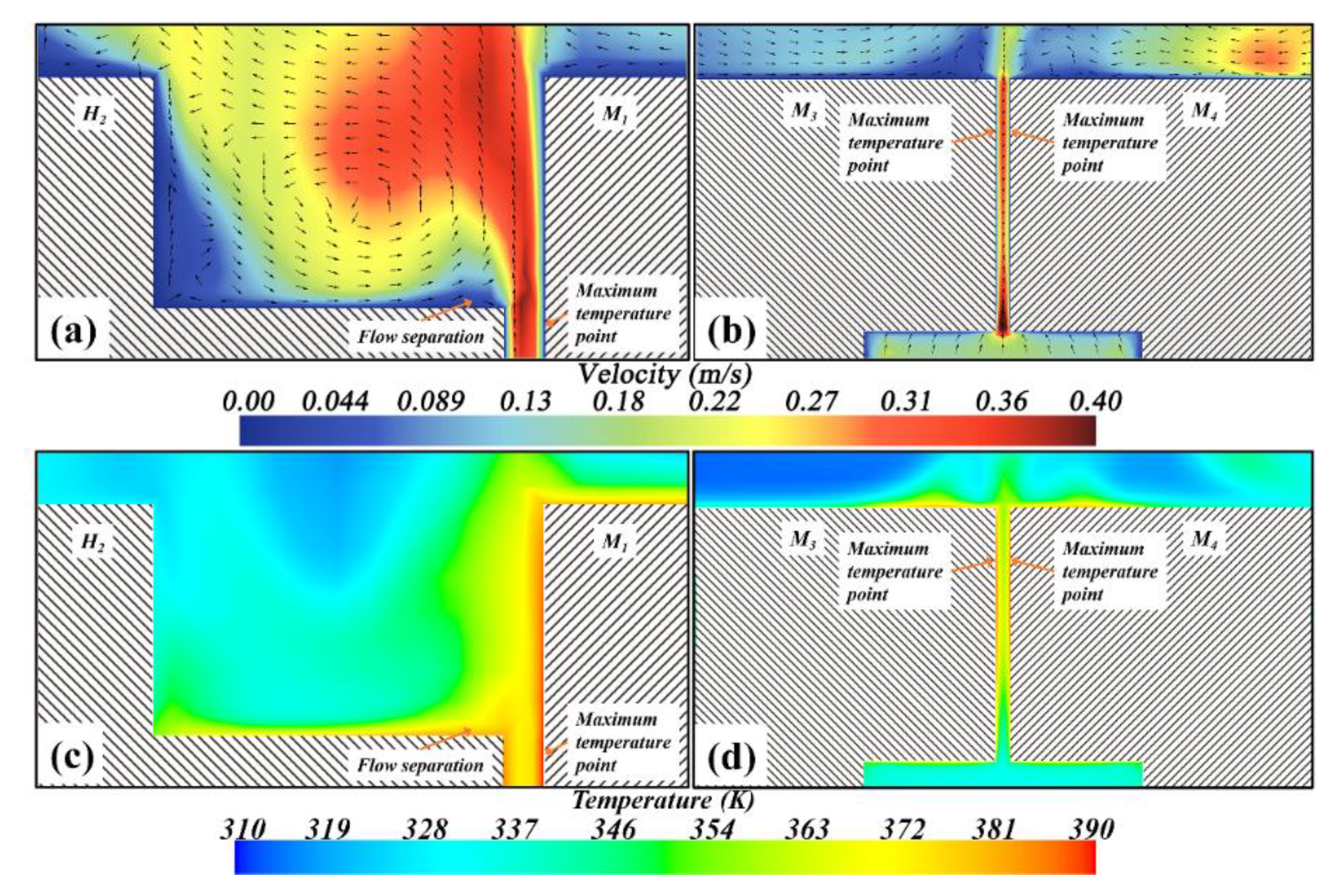
Figure 4.
Surface temperature contour of M6 under different vacuum levels at different heating stage: (a) 3 min heating under 0.1 atm; (b) 3 min heating under 0.3 atm; (c) 3 min heating under 1.0 atm; (d) 10 min heating under 0.1 atm; (e) 10 min heating under 0.3 atm; (f) 10 min heating under 1.0 atm; (g) 60 min heating under 0.1 atm; (h) 60 min heating under 0.3 atm; and (i) 60 min heating under 1.0 atm.

Figure 5.
Velocity contour of flow field on the symmetric plane of levitation electromagnets module after 60 min heating: (a) Vacuum level: 0.1 atm; and (b) Vacuum level: 1.0 atm.
Figure 5.
Velocity contour of flow field on the symmetric plane of levitation electromagnets module after 60 min heating: (a) Vacuum level: 0.1 atm; and (b) Vacuum level: 1.0 atm.
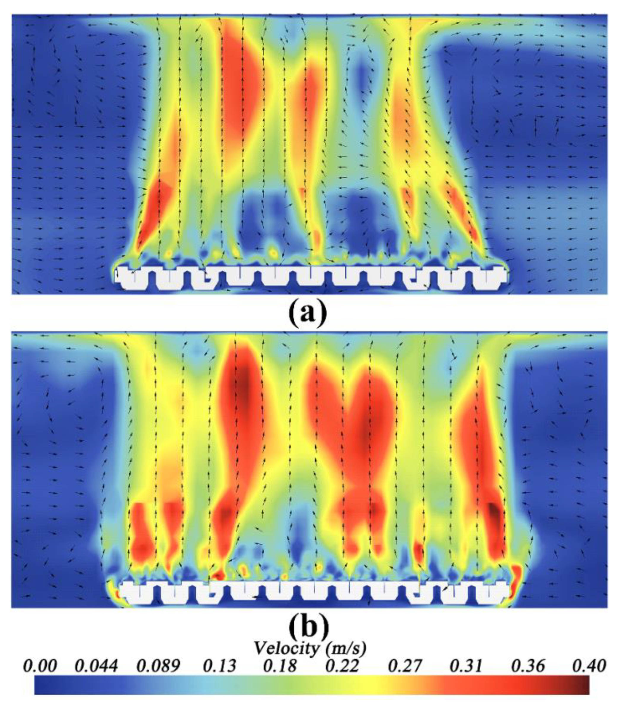
Figure 6.
Distribution of temperature and temperature gradient in the fluid domain along the surface’s outer-normal direction of point Pd at different vacuum levels: (a) Temperature diagram; (b) Temperature gradient diagram.
Figure 6.
Distribution of temperature and temperature gradient in the fluid domain along the surface’s outer-normal direction of point Pd at different vacuum levels: (a) Temperature diagram; (b) Temperature gradient diagram.

Figure 7.
Maximum temperature rise on EMU surface under different vacuum levels during heating process.
Figure 7.
Maximum temperature rise on EMU surface under different vacuum levels during heating process.
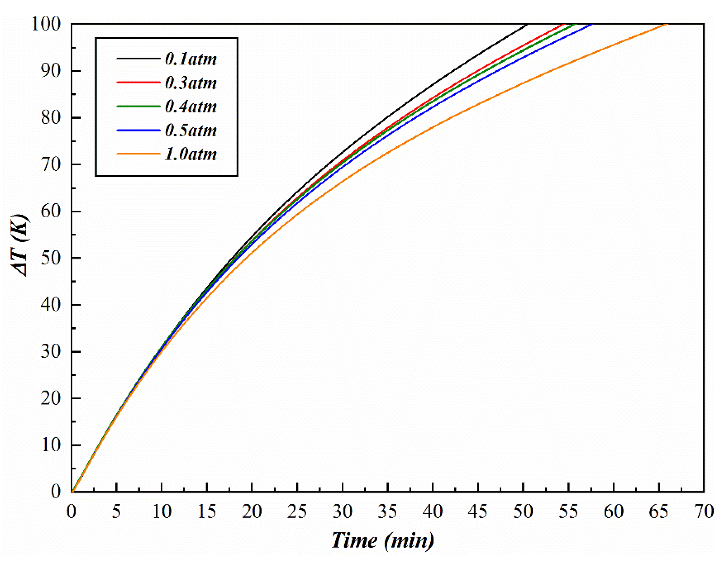
Figure 8.
Average convection heat flux on the levitation electromagnet surface.
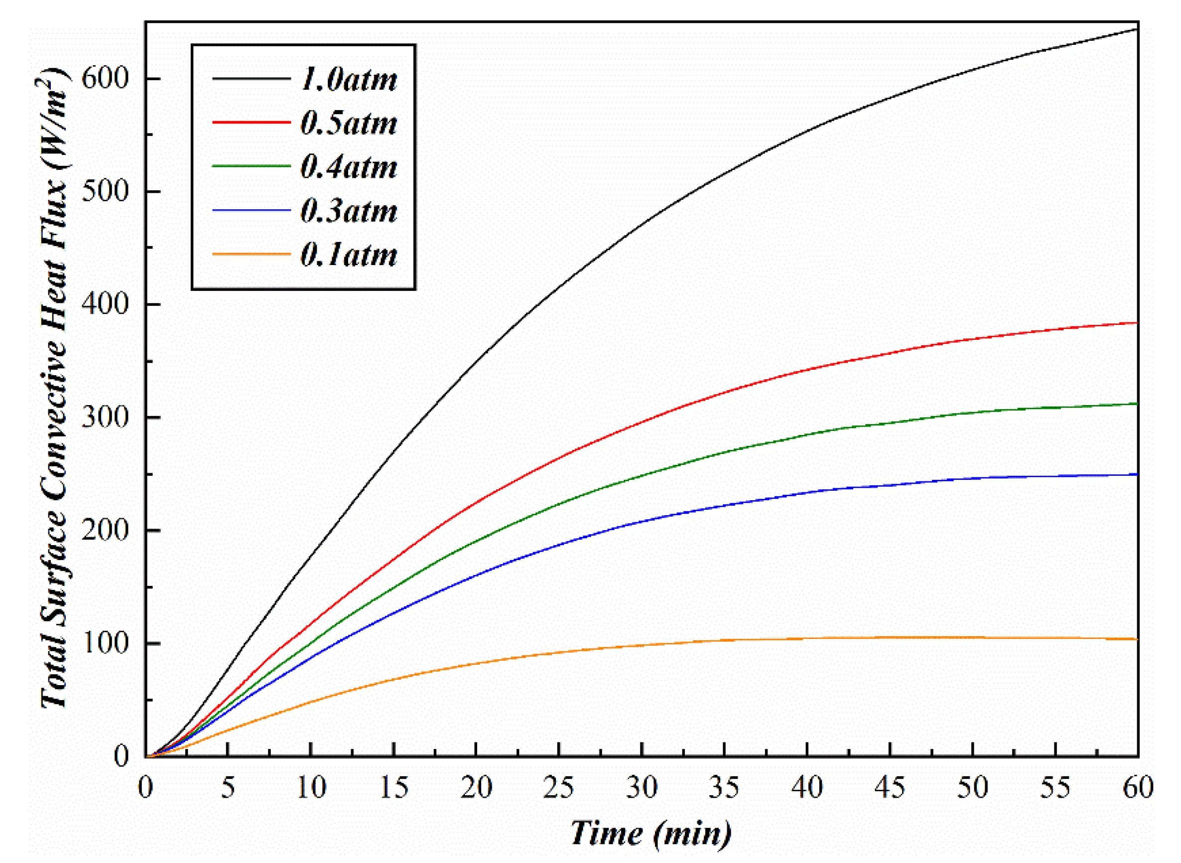
Figure 9.
Weight of convection heat flux over the total heat flux on the fluid–solid interface during the heating process.
Figure 9.
Weight of convection heat flux over the total heat flux on the fluid–solid interface during the heating process.
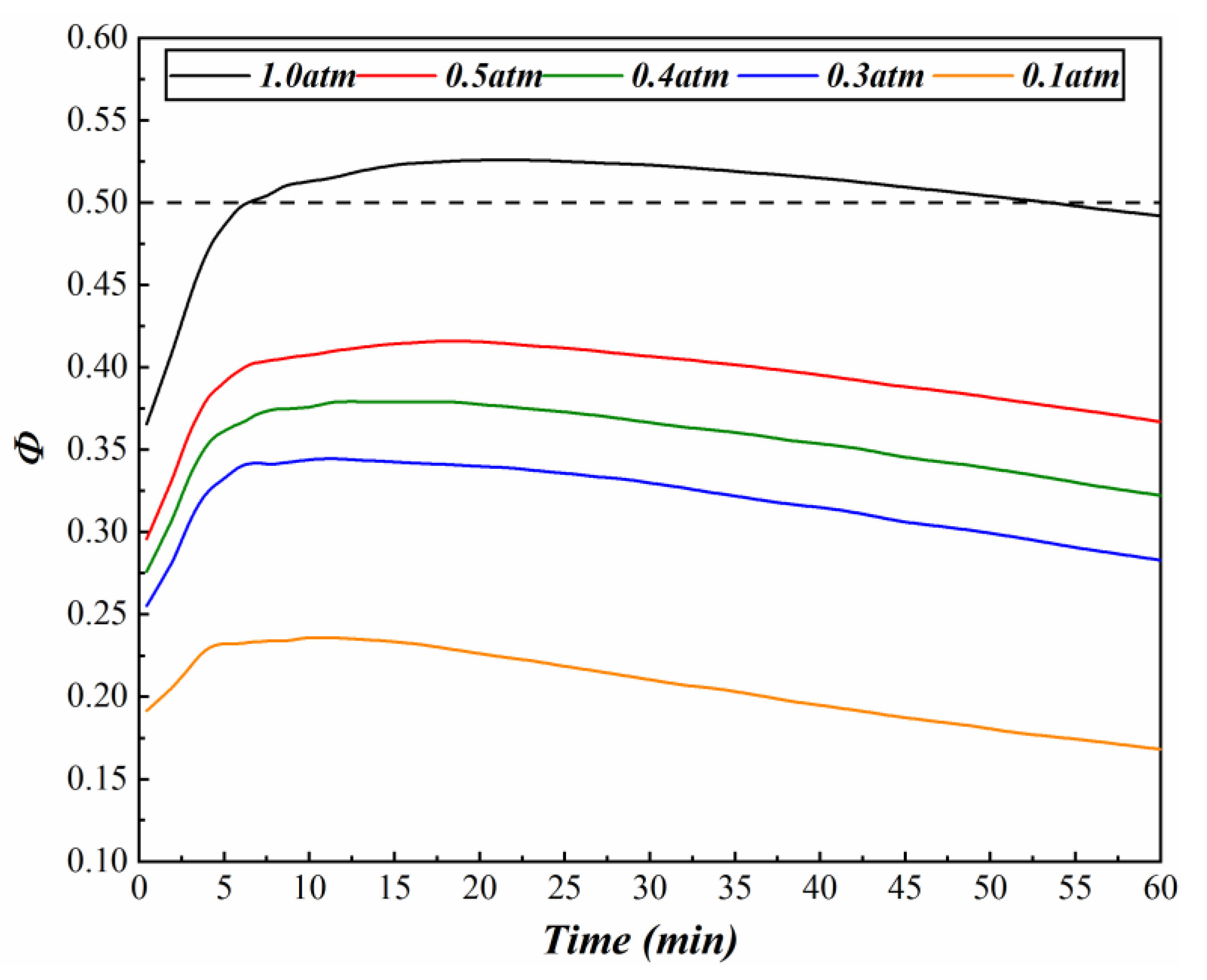
Figure 10.
Relationship between accumulated heat through the magnet surface and vacuum level: (a) Total heat; (b) Convection heat.
Figure 10.
Relationship between accumulated heat through the magnet surface and vacuum level: (a) Total heat; (b) Convection heat.
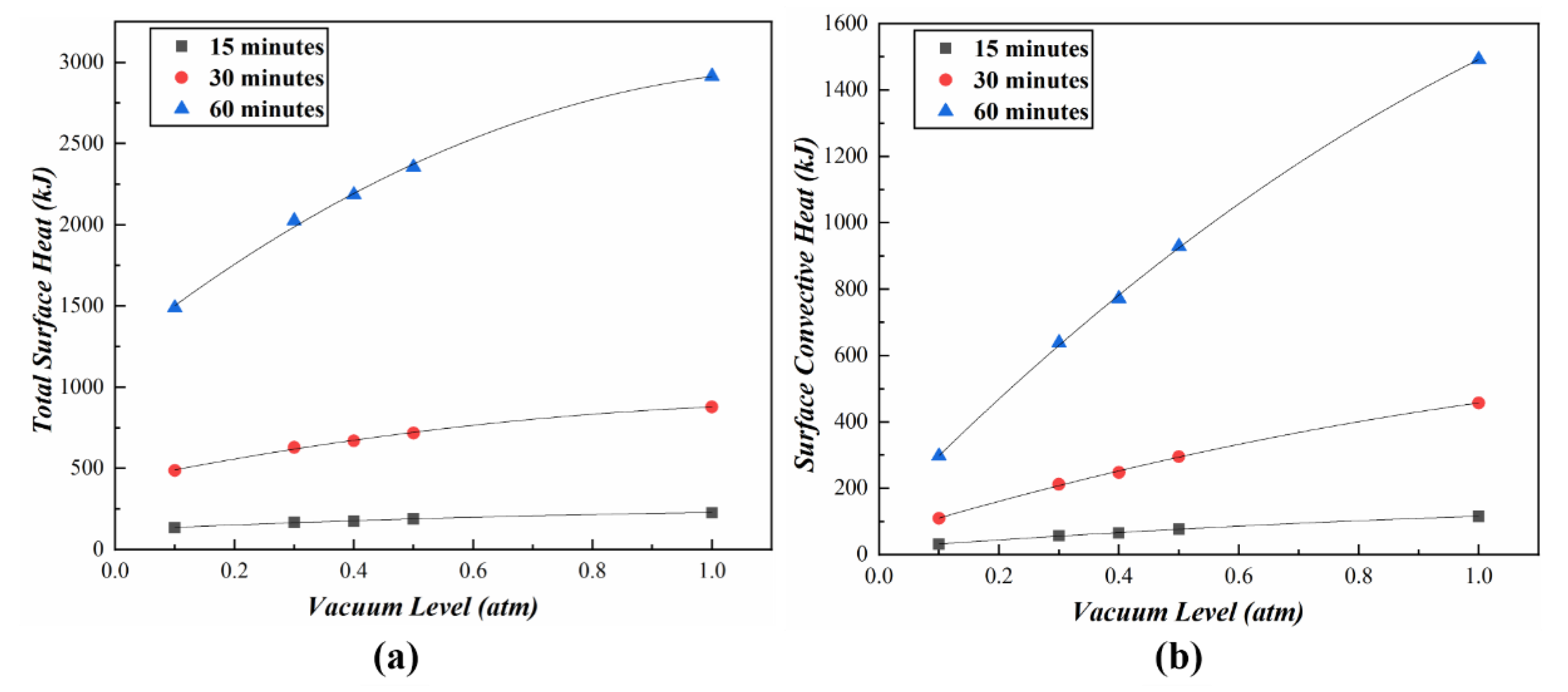
Figure 11.
Influence of vacuum level on effective convection heat transfer coefficient () of EMUs.

Table 1.
Physical parameters of solid components.
| Component | Density | Heat Capacity | Thermal Conductivity | Heating Power Per Volume | |
|---|---|---|---|---|---|
| (kg/m3) | J/(kg·K) | (W/(m∙K)) | (kW/m3) | ||
| Coils | 2554 | 832.5 | 3.6 | Primary magnet units and core-elevated magnet units | 154 |
| End magnet units | 152 | ||||
| Iron core | 7450 | 430 | 17 | 0 | |
| Epoxy | 1150 | 2410 | 0.4 | ||
| Flange | 2800 | 880 | 160 | ||
| Glass fiber | 2600 | 670 | 0.4 | ||
Table 2.
Parameters and results in mesh sensitivity study.
| Coarse | Medium (Segregated Solver) | Medium (Coupled Solver) | Fine | Experiment | ||
|---|---|---|---|---|---|---|
| Total number of grids (million) | 2.94 | 10.03 | 10.03 | 47.82 | / | |
| Temperature rise during heating process (K) | 10 min | 30.66 | 30.26 | 30.25 | 30.16 | 24.6 |
| 20 min | 52.99 | 52.65 | 52.62 | 52.55 | 47.63 | |
| 30 min | 69.37 | 69.02 | 68.98 | 68.93 | 65.91 | |
| 40 min | 82.28 | 82.04 | 82.02 | 81.99 | 80.14 | |
| 50 min | 93.25 | 93.11 | 93.1 | 93.09 | 93 | |
| 60 min | 101.72 | 102.21 | 102.25 | 102.41 | / | |
| 100 K temperature rise time (min) | 58.6 | 58.2 | 58.1 | 57.9 | 57.0 | |
| Heating time difference (%) | 2.8 | 2.1 | 1.9 | 1.6 | / | |
Table 3.
Maximum surface temperature rise on different type of electromagnet units (EMUs) under 1.0 atm.
Table 3.
Maximum surface temperature rise on different type of electromagnet units (EMUs) under 1.0 atm.
| Heating Time (min) | 10 | 20 | 30 | 40 | 50 | 60 |
|---|---|---|---|---|---|---|
| Primary magnet units | 30.1 | 51.3 | 66.5 | 78.0 | 87.4 | 95.6 |
| Core-elevated magnet units | 30.4 | 50.9 | 65.3 | 76.3 | 85.7 | 94.0 |
| End magnet units | 29.9 | 50.0 | 64.5 | 76.1 | 86.0 | 95.0 |
Table 4.
Maximum temperature rise of each primary magnet unit after 60 min heating under 1.0 atm.
| Primary Magnet Units ID | M1 | M2 | M3 | M4 | M5 | M6 |
|---|---|---|---|---|---|---|
| (K) | 95.6 | 94.1 | 93.9 | 93.9 | 94.0 | 95.6 |
Table 5.
100 K temperature rise process at different vacuum levels.
| Vacuum Level (atm) | 0.1 | 0.3 | 0.4 | 0.5 | 1.0 |
|---|---|---|---|---|---|
| Temperature rise time (min) | 50.5 | 54.4 | 55.7 | 57.6 | 66.0 |
| Heating time difference (compared to heating under 1.0 atm, %) | 23 | 18 | 16 | 13 | / |
Table 6.
Appearance time of inflection point in Figure 9.
Table 6.
Appearance time of inflection point in Figure 9.
| Vacuum Level (atm) | 0.1 | 0.3 | 0.4 | 0.5 | 1 |
|---|---|---|---|---|---|
| Time (min) | 10.9 | 11.3 | 17.2 | 18.3 | 21.0 |
Table 7.
Effective convection heat transfer coefficient of the EMU under different vacuum levels.
| Vacuum Level (atm) | 0.1 | 0.3 | 0.4 | 0.5 | 1 |
|---|---|---|---|---|---|
| he (W/(m2∙K)) | 0.44 | 1.37 | 1.80 | 2.27 | 4.11 |
© 2020 by the authors. Licensee MDPI, Basel, Switzerland. This article is an open access article distributed under the terms and conditions of the Creative Commons Attribution (CC BY) license (http://creativecommons.org/licenses/by/4.0/).
Share and Cite
MDPI and ACS Style
Mao, Y.; Yang, M.; Wang, T.; Wu, F.; Qian, B. Influence of Vacuum Level on Heat Transfer Characteristics of Maglev Levitation Electromagnet Module. Appl. Sci. 2020, 10, 1106. https://doi.org/10.3390/app10031106
AMA Style
Mao Y, Yang M, Wang T, Wu F, Qian B. Influence of Vacuum Level on Heat Transfer Characteristics of Maglev Levitation Electromagnet Module. Applied Sciences. 2020; 10(3):1106. https://doi.org/10.3390/app10031106
Chicago/Turabian StyleMao, Yiqian, Mingzhi Yang, Tiantian Wang, Fan Wu, and Bosen Qian. 2020. "Influence of Vacuum Level on Heat Transfer Characteristics of Maglev Levitation Electromagnet Module" Applied Sciences 10, no. 3: 1106. https://doi.org/10.3390/app10031106
Note that from the first issue of 2016, this journal uses article numbers instead of page numbers. See further details here.