Driving Safety Improved with Control of Magnetorheological Dampers in Vehicle Suspension


Department of Measurements and Control Systems, Silesian University of Technology, Akademicka 16, 44-100 Gliwice, Poland
*
Author to whom correspondence should be addressed.
Appl. Sci. 2020, 10(24), 8892; https://doi.org/10.3390/app10248892
Submission received: 24 November 2020
/
Revised: 10 December 2020
/
Accepted: 10 December 2020
/
Published: 12 December 2020
(This article belongs to the Special Issue Friction and Impact-Induced Vibration)
Abstract
:The article is dedicated to the control of magnetorheological dampers (MR) included in a semi-active suspension of an all-terrain vehicle moving along a rough road profile. The simulation results of a half-car model and selected feedback vibration control algorithms are presented and analysed with respect to the improvement of driving safety features, such as road holding and vehicle handling. Constant control currents correspond to the passive suspension of different damping parameters. Independent Skyhook control of suspension parts represents the robust and widely used semi-active algorithm. Furthermore, its extension allows for the control of vehicle body heave and pitch vibration modes. Tests of the algorithms are carried out for a vehicle model that is synthesised with particular emphasis on mapping different phenomena occurring in a moving vehicle. The coupling of the vehicle to the road and environment is described by non-linear tire-road friction, rolling resistance, and aerodynamic drag. The pitching behaviour of the vehicle body, as well as the deflection of the suspension, is described by a suspension sub-model that exhibits four degrees of freedom. Further, three degrees of freedom of the complete model describe longitudinal movement of the vehicle and angular motion of its wheels. The MR damper model that is based on hyperbolic tangent function is favoured for describing the key phenomena of the MR damper behaviour, including non-linear shape and force saturation that are represented by force-velocity characteristics. The applied simulation environment is used for the evaluation of different semi-active control algorithms supported by an inverse MR damper model. The vehicle model is subjected to vibration excitation that is induced by road irregularities and road manoeuvres, such as accelerating and braking. The implemented control algorithms and different configurations of passive suspension are compared while using driving-safety-related quality indices.
1. Introduction
The driving safety of road and off-road vehicles is the key feature that allows for safe and reliable transportation of passengers and different types of loads. Driving safety is a broad concept; here, it mainly refers to road holding and vehicle handling varying with respect to different configurations of vehicle suspension.
Road holding describes the ability of the vehicle to track the desired road trajectory and it can be influenced by different factors. Each tire and vehicle exhibits its optimized window of tire inflation, or tire deflection, which has a similar, but opposite, effect. Studies on inflation of tire were discussed in [1,2], where the typical deformation of underinflated tire was presented. Further analysis of non-uniform contact stress distribution for over and underinflated tire was presented in [3].
Both under and overdeflected tires result in accelerated tire wear and the deterioration of tire adhesion to road surface. Furthermore, not only static, but also dynamic changes in tire deflection should be taken into account [4]. The latter can be significantly increased by a wheel hop effect, which is related to the resonance of vehicle wheel vibration.
Vehicle handling, the second driving-safety-related feature, is commonly evaluated for steady-state or transient response of the vehicle, as shown in [5]. The steady-state response was analysed for a vehicle moving along a circle with increasing speed. Transient tests can be closed-loop, e.g., severe double line change or open-loop, e.g., J-turn, Fishhook. Further, vehicle handling can be analysed with respect to the chance of vehicle rollover.
An indicator of a possible rollover that was evaluated based on measurement data of roll angle and additional information about vehicle kinetic energy was presented in [6]. Other researchers proposed the roll rate as quantity that is related to the likelihood of rollover [4]. Consequently, pitch angle can also be used for the assessment of ride performance and steering stability as it was stated in [7]. Further, the approach of assessing vehicle handling on the pitch and roll rates was also applied in [8], presenting an analysis of whole body vibration for an off-road vehicle with magnetorheological (MR) dampers.
1.1. Vehicle Suspension
The parameters of the passive suspension can be optimized in terms of driving safety, but it is associated with a reduction in driving comfort. This statement was confirmed in [5] with respect to different cases that indicate that suspension settings for spring and damper parameters corresponding to ride comfort or driving safety are contradictory. Parameters of commonly used passive suspension are hard to change after being manufactured and they are dedicated to certain vehicle destination, e.g., road and off-road vehicles or sports cars. However, still, varying road conditions require the suspension parameters to be constantly adapted.
Active suspension systems are equipped with force generators that can effectively improve ride comfort and driving safety, as presented in [9], where the control methods for slow-active suspension were described. However, the high energy consumption of active suspension elements is their key disadvantage and is still an urgent problem described in the literature. The same authors presented, in [10], a study on energy consumption of an active suspension and proposed a weighted multitone optimal controller in order to minimise this consumption while the application of the ideal energy harvester was also analysed.
The application of a less energy-consuming semi-active suspension is a competitive offer. The operation of semi-active suspension dampers, especially magnetorheological dampers, is based on control of dissipation of vibration energy. They can also offer a short time response studied in [11], which is critical in vibration control applications. The authors presented an experimental analysis of the MR damper response time and showed that, in most cases, the response time to step current excitation does not exceed 20 milliseconds. It is worth noting that, similarly to active solutions, semi-active dampers are also supported by an energy harvester, which further improves the performance of semi-active approach. For instance, a novel design of the MR damper was presented in [12], where a controllable damping mechanism was integrated with a converter of mechanical energy to electrical energy.
Force-velocity characteristics of MR damper are strongly nonlinear, and they include hysteresis loops and force saturation regions [13]. Numerous models of MR damper were presented in the literature, including the Bingham model based on Coulomb force and viscous damping components [13]. A key element of the Spencer–Dyke model presented in [14] is a Bouc–Wen hysteresis component that was described by a nonlinear differential equation. The advantage of the MR damper model, which is based on hyperbolic tangent function, as presented in [15], is its simple form and good fit to the force-velocity experimental characteristics of MR damper. Furthermore, this model can be easily inverted, which is favorable in the case of control applications.
1.2. Modelling of the Vehicle
Numerous studies that are presented in the literature are devoted to simulation research that precede work on prototyping and commercial applications of MR dampers. They usually represent some kind of compromise between the accuracy of modelling and the requirement of simplicity of solutions, because, in the next stage, the developed control algorithm should be implemented in the microcontroller. Moreover, the use of very complex vehicle models requires the design of appropriate experiments in order to identify a large number of parameters, especially when it is necessary to take the measurement uncertainty into account [16].
Models of suspension are commonly grouped into a quarter-car, half-car, or full-car models. The quarter-car model is recommended when an initial analysis of the mechanical system is performed. Furthermore, it allows for a simple demonstration of control algorithm, like e.g., Skyhook control [17]. Half-car model is recommended when the pitch or roll dynamics of vehicle body have to be analysed, e.g., minimisation of quantities that are related to both ride comfort or driving safety while using H-infinity optimal control was presented in [18]. The full-car suspension model, which usually exhibits seven degrees of freedom, takes into account the vertical motion of the wheels, as well as heave, pitch, and roll motion of the body [19].
The next problem that should be taken into account is how to model a wheel. Usually, for the purpose of vehicle dynamics simulation the wheel is decomposed into the rim and tire. Depending on the model complexity vertical motion only or additionally lateral and rotational motion of the rim can be included in the wheel model. The dynamics of the rim depends on several factors, i.e., force and torque that are exerted by the road surface, as well as torques that are generated by the drive and braking system.
The modelling of tire behaviour during the ride is complex due to the susceptibility of rubber to large deformations. The complex tire structure is a second reason, where several elements of tire can be distinguished, e.g., tire treads, belt, sidewalls, or bead bundle [2]. Different phenomena are observed for the driving tire, such as longitudinal and lateral stiffness and damping, rolling resistance, or significantly nonlinear tire friction on the road. In [20], it was stated that four categories of possible approaches for developing a tire model can be distinguished, i.e., based on experimental data only, using similarity methods, based on a simple or more complex physical model.
The vertical tire model (i.e., the tire dynamics is considered vertically) that is presented in [21] is the simplest and most widely used in research. Further, the model can be extended by longitudinal or lateral forces [2]. Also, a group of radially and circumstantially located dampers and springs can be used. The most complex tire models are described using final element methods (FEM), as it was shown in [22,23], where modal analysis for steady or rolling tire was performed or circumferential waves at wheel’s critical speed were considered [2]. Other types of models allow for precise analysis of interactions between tire and road, as in the case of FEM models [24] or based on evaluation of contact mechanics between tread blocks and road surface [23]. Moreover, an alternative analytical model of the tire was applied in [25] in the case of uneven roads.
Rolling resistance is observed for rolling objects, while it is especially noticeable in the case of elastic tire where the energy for the expanding tire on the rear of the wheel is not fully restored, but dissipated. It results in a non-uniform distribution of ground normal stress, more generally, the resultant ground reaction force is shifted forward with respect to tire contact patch, as shown in [26,27] or [2]. It results in reaction force, which not only acts on the wheel center of gravity, but also generates a braking torque for the tire. The rolling resistance can be described by the shift of reaction force, but is more often normalized by the effective radius of the wheel resulting in a rolling resistance coefficient, which depends on several factors in a closer analysis, e.g., ambient temperature, types of road and tire materials, vehicle speed, tire air pressure, and vehicle load.
Interaction between tire and road profile is mainly based on phenomena such as rubber hysteresis that is caused by its continuous compression and expansion and a rubber adhesion to the road surface, as shown in [21] or [2]. The parameters of this interaction are significantly dependent on the condition of the road, e.g., wet, dry, or snow-covered road. Many researchers have analysed the behaviour of tire rubber, e.g., rubber friction was measured while using a dedicated test machine for different types of surface in [28].
Behaviour of tire rubber is being generalized and simplified for implementation in simulation and control applications. The Brush model (or Bristle model) described, e.g., in [26,27,29,30] or [20], corresponds to the tire model, where the rubber can be approximated as small elements of brush, where every element can bend independently.
In order to further simplify the analysis of vehicle dynamics with respect to tire-road friction, a relationship between slip ratio and the friction force is considered, where the former is defined as the ratio between the relative slip velocity and absolute longitudinal velocity of the wheel. The characteristics of friction force to slip ratio can be divided into three regions, i.e., elastic or linear region, transitional region, and frictional region [31]. Further, a semi-empirical models are widely used in the literature which describe the friction-slip characteristics by mathematical functions, e.g., Magic Formula tire model presented in [20].
The Burckhardt model presented in [32], which was further reviewed in [33], or the Reimpell model that was described in [34], are also semi-empirical tire models known in the literature. In the case of Burckhardt model, the longitudinal slip force is evaluated in the direction of wheel motion, while, in the case of Reimpell model, the slip force is derived in the direction of wheel orientation. Finally, a Fiala tire model is presented in [21], which is widely used in simulation, e.g., MSC ADAMS, assumes that each element of the surface can be displaced from its initial position and counteract with an assumed stiffness parameter.
1.3. Control of Semi-Active Suspension
Control algorithms that are dedicated to MR dampers are usually decomposed into the lower force control layer and the upper vibration control layer. The force control can operate in the open or closed loop. The open-loop takes advantage of the invertible MR damper model, while the closed-loop approach requires a force feedback signal. Force measurements are widely used in mechanical system starting from small-scale elements of vehicle suspension [35] to strain gauge that can be applied in mechanical constructions from suspension to a large-scale bridge conveyor of bucket wheel excavator [36].
The application of MR dampers in vehicle suspension allows for changing the suspension settings from soft to hard during the drive. However, the Skyhook algorithm that is presented in [17] is considered as one of the first semi-active control algorithms, simultaneously robust and widely tested, e.g., in [8] for an all-terrain vehicle (ATV). It also serves as a reference for other algorithms. On the other hand, the Groundhook algorithm described, e.g., in [37] generates a desired force that is inversely proportional to the wheel vertical velocity, whereas Skyhook generates force that is related to the vertical velocity of the body.
Applications of MR dampers can be also limited to the suppression of a seat vibration only. The real-time control of the MR damper applied for a driver seat with on-off and continuously variable control was presented in [13]. Further, the results of vibration suppression for an operator cabin in bucket wheel excavators were presented in [38], where the authors proposed an iterative learning method for optimal control.
Fuzzy control serves as an alternative control approach that can be applied for MR dampers [39], where an inverse MR damper is not required. Other authors presented, in [40], a control system of a vehicle model with MR dampers that was integrated with braking and front steering subsystems. Here, the study is more complex and takes into account both suspension dynamics and tire-road interaction in the form of a Magic Formula tire model. However, the authors focused their study on vehicle vibration that was induced by road manoeuvres, while road irregularities as well as the vertical dynamics of the wheel were not taken into account.
1.4. Highlights
The studies presented in the literature and related to vehicle vibration control using magnetorheological dampers are commonly limited to stationary vehicle suspension model, which does not take the longitudinal motion of the vehicle, more complex wheel model, or tire to road friction into account. Typically, description of tire-road interaction is limited to their contact in a single point. Admittedly, sophisticated models of vehicle and tire dynamics are well known; however, they are rarely related to semi-active suspension and semi-active control algorithms, in particular with regard to the analysis of road holding and vehicle handling.
The presented study discusses the interaction between the road surface and half-car vehicle model equipped with MR dampers and controlled with standard semi-active control algorithms. The most important phenomena that may occur while driving are taken into account, such as tire slip, body heave and pitch motion, wheel vibration, rolling resistance, and aerodynamic drag. It was shown how the suspension control influences the vehicle behaviour during the typical driving phases, i.e., accelerating, driving with constant speed, and braking.
The results were obtained for a vehicle model, which is, in detail, referred to an actual, commercially available, and real-size all-terrain vehicle (ATV), which was additionally equipped with suspension MR dampers. The road profile was generated according to the norm ISO 8608 describing road surface profiles with respect to mechanical vibration [41]. Furthermore, the influence of road profile on the vehicle wheel was evaluated while assuming the actual parameters and dimensions of the ATV’s wheels.
The methodology of road holding and vehicle handling was proposed while road holding was further analysed with respect to susceptibility of the wheels to separation from the road surface and fluctuations of the normal force exerted by the ground. It was also shown that driving-safety-related studies, like other research areas, require statistical analysis and averaging operation performed over several realizations. It is caused by the fact that the effective influence of the road on wheels depends on many factors, including applied control algorithms, tire and suspension deflection, or vehicle speed, despite the fact that the same road profile was used.
The paper is organized, as follows. Section 2 presents the description of the vehicle model, including the method of generating the road profile, a half-car submodel of vehicle suspension, and the MR damper model, which is based on a hyperbolic tangent function. The distributed model of tires takes into account the averaged normal force exerted by the ground and damping related to the tire deflection.
Further, the interactions of the vehicle with the road and slipping effect are described by the Burckhardt model of tire-road friction. The description of wheels dynamics includes their moment of inertia, which has influence on effective torques that are generated by the rear drive system and disc brake on the front wheel, similarly as in the real vehicle. The model of wheels also includes rolling resistance while the whole vehicle is subjected to aerodynamic drag.
Section 3 is dedicated to semi-active suspension control algorithms in which three control approaches are compared. First, a case of MR dampers controlled by different values of constant current is defined, which reflects different soft and hard configurations of passive suspension. Further, two variants of Skyhook control are presented, where the former is based on separate control of suspension parts, while the latter emulates different damping forces that are exerted on heave and pitch velocities of the vehicle body.
Section 4 presents the results obtained for implemented semi-active control approaches with respect to road holding and vehicle handling. Three phases of a typical drive were distinguished, i.e., accelerating from vehicle stop, driving at a constant speed assumed as set by an external object and braking until the vehicle stops. In the case of the road holding, the given algorithms were mainly compared with respect to their ability to avoid detachment from the road, which is evaluated as the weighted mean value of normal wheel forces.
The normal forces were also studied in frequency domain based on power spectral density (PSD) characteristics. Further, vehicle body and wheels were also analysed, as well as the occurrence of slip is observed. The second part of this section is dedicated to vehicle handling, which is analysed based on mean values and standard deviations of vehicle body pitch velocity evaluated similarly for different drive phases. Section 5 provides the conclusions of study dedicated to driving safety of ATV with MR dampers.
2. Vehicle Model and Its Coupling with Road and Environment
The presented results refer to the actual, commercially available ATV-Sweden that is shown in Figure 1a, manufactured by CF-Moto. According to the vehicle approval documents, it is 2.185 m long, 1.17 m wide, 1.23 m high, and its mass is approximately 393 kg.
Original shock-absorbers have been replaced with MR suspension dampers. It is also worth noting that each part of the suspension operates independently, which allows for only adapting a selected MR damper to the road unevenness. The vehicle is equipped with a measurement and control system in order to generate appropriate control currents for MR dampers.
The measurement part of the system includes numerous sensors. Mainly, three-axis accelerometers are used. Five of them are located in the vehicle body and additional accelerometers are located in the vicinity of each wheel. Furthermore, the deflection of each suspension part is measured while using an LVDT (linear variable differential transformer). Pitch and roll motion of the body, as well as acceleration of the driver’s seat, are measured by the additional IMU (inertial measurement unit). The angular velocity of each wheel can be roughly measured while using a Hall effect sensor and numerous neodymium magnets that are attached to the wheel rim. Regardless of this, the speed of the vehicle is measured by the standard sensor.
The study is focused on the analysis of longitudinal behaviour of the vehicle model during accelerating, braking or driving with a constant speed. Thus, simulation was performed for a half-car model which describes the major behaviour of the vehicle during road manoeuvres mentioned above, i.e., longitudinal and vertical motion as well as body pitch. The parameters that were used for the model simulation were carefully estimated and listed further in Table 1 in Section 4. The proposed half-car model exhibits seven degrees of freedom (DoFs) and its graphical representation is shown in Figure 1b. First four DoFs are related to wheel vertical and angular motion, denoted as and for the front wheel, respectively, as well as and corresponding to the rear wheel. Further two DoFs, denoted as and , describe the heave and pitch motion of the body, respectively. For the simplification of the model, an assumption was made that longitudinal displacements of all vehicle components are the same and they are depicted by the last DoF, denoted as .
This model describes the dynamics of the half of the vehicle. Thus, selected vehicle parameters, e.g., mass or moment of inertia of the body as well as the torque of the drive system need to be scaled down. The wheel weights were measured as = 10 kg and = 15 kg for the front and rear wheel, respectively. Half of the body weight is = 171.5 kg while taking the weights of the wheels into account. Longitudinal location of the body centre of gravity (CoG) was estimated and defined by = 0.609 and = 0.681 m, which show that CoG is slightly shifted toward the front of the vehicle. The height of the vehicle CoG = 0.554 m was taken from the literature [42], where the selected parameters of the CF500 vehicle are listed.
Any data related to the body moment of inertia are hardly available for this type of vehicle, while experimental identification is not a trivial task for such weight. Therefore, moment of inertia of the body was estimated as = 74.3 kgm for and assuming a uniform distribution of the body mass, which vertically starts at a height of 0.25 and ends at a height of 0.9 m.
The stiffness parameters of the suspension were obtained as = 22,208 Nm and = 34,857 Nm for the front and rear suspension, respectively, based on measurements of stiffness performed separately for suspension springs while using a material testing system (MTS) dedicated to static tests. Passive damping parameters were coarsely assumed as = = 300 Nsm, the same for the front and rear part. Furthermore, it should be noted that the applied MR dampers are a dominant source of suspension damping, and they were carefully examined while using MTS dedicated to dynamic tests. Section 2.6 discusses their model.
2.1. Road Profile
Random road profile exhibits an integral character according to the norm ISO 8608 [41], i.e., low frequency components of the road profile present greater amplitudes and vice versa. Thus, the spatial power spectral density (PSD) of an ideal road profile, denoted as , can be described with respect to the spatial angular frequency as follows:
where is a reference value of that is dedicated to a selected road class at an angular frequency = 1. Here, class F is used in order to reflect off-road conditions; thus, = = was assumed. The value of was set as the geometric mean of the range for class F. Figure 2b presents the resultant characteristics of evaluated with respect to the spatial frequency as well as the simulated road profile.
The generation of road profile was realized by filtering a Gaussian white noise dependent on the distance coordinate x while using an integrating digital discrete-distance filter of transfer function . A continuous-distance filter equivalent to was defined in order to more clearly discuss its parameters and relate them to the continuous-distance spatial PSD :
where = 6.6 m is a cutoff wavelength (an equivalent of time constant in the time domain, noticeable for low frequencies in Figure 2b), which is much greater than the wheelbase of the vehicle equal to 1.29 m. Consequently, Figure 2a shows a diagram of a sample road profile with respect to distance.
The filtering of white noise can only be accomplished in the discrete domain, since white noise cannot be realized in reality. Besides, the resolution of the generated road profile was assumed as = 1000 points per meter. Thus, a discrete realization of white noise was used with variance in order to obtain a unit level of the input random signal in spatial PSD , defined with respect to .
Higher spatial frequencies of the generated road profile can be neglected in further analysis due to the much greater dimension of wheels. Furthermore, the road profile needs to be differentiated in order to obtain indicating an inclination of road in a given point, which is required by the vehicle simulator. Thus, the bandwidth of the road profile was limited to the cutoff spatial frequency that was equal to 200 cycles per meter (see Figure 2b) while using an additional discrete domain finite impulse response filter (FIR).
2.2. Wheel and Tire Model
The experimental ATV is equipped with two types of wheels of different widths that were equal to = 0.2 m (8 inches) for the front wheel and = 0.254 meter (10 inches) for the rear wheel. Other dimensions of both wheels remain the same, i.e., radius of the unloaded wheel = = 0.317 m and radius of the rim = = 0.152 m (6 inches).
A tire aspect ratio being a ratio of tire sidewall height to tire width is a key parameter defining a type of tire. For standard tires, this ratio varies commonly from 0.5 to 0.7. In the experimental vehicle, this parameter takes a value of 0.65 for the rear tire and 0.81 for the front. Thus, the front tire appears to be slimmer in comparison to standard tires and the rear wheel is assumed as a reference in order to estimate moment of inertia of both wheels, denoted as and , respectively.
The diagram of the moments of inertia of the wheels for standard vehicles was presented with respect to a dynamic wheel radius (i.e., for a moving vehicle) in [43]. These data were compiled for the purpose of this study with a comparison between the dynamic radii and radii of unloaded wheels that were obtained experimentally and discussed in [44]. Consequently, the moment of inertia of the standard rear wheel was evaluated as = 0.9 kg m with respect to the aspect ratio. The moment of inertia of the front wheel was scaled down with respect to the ratio between wheel weights and evaluated as = 0.6 kg m, since the moment of inertia depends on a weight of the object with the same shape and size of the cross-section.
The goal of the tire model is to evaluate the resultant force and torque acting on the wheel axle at a given time instant. These forces are related to ground force generated as a reaction to tire stiffness and damping forces in a given point of road profile, as noted in Figure 3. The tire stiffness comes mainly from the compressed air of pressure inside the tire, which acts on a road surface. Tire damping is defined here as a force which counteracts deflection of the tire and is directly proportional to the velocity of deflection denoted as . Ground forces are transferred through the stiff sidewalls of the tire to the wheel axle. The rim was assumed as a rigid component, while the outer surface of the tire is assumed to be deformable, ideally adapting to uneven terrain.
The evaluation of wheel forces is performed in several stages for a given moment in time. Firstly, for a given location of wheel and known road profile an area of tire cross-section, denoted as , is calculated, which shows how much the road deflects the tire. Next, instantaneous tire air pressure multiplied by is calculated according to the general gas Clapeyron’s equation assuming a constant temperature:
where denotes an initial area of tire air and it is equal to the difference of wheel and rim areas. Symbol denotes initial tire air pressure, while the method of its estimation multiplied by is later described in the subsection. The instantaneous area of tire air is denoted as .
Stiffness and damping forces that are generated by each fragment of the road profile contribute to the resultant force and in x and z directions, respectively, as well as torque , as follows:
where angle describes orientation of radius with respect to the vertical axis. Angle denotes an inclination of the road profile in the given point and it can be calculated based on a derivative of the road profile height with respect to its coordinate . The forces that are presented in Equation (4) are calculated for the road surface coordinates varying from to , which is the radius of unloaded wheel. Using the max function means that Equation (4) is only considered for not lower than zero, which indicates detachment from the road surface. The wheel radius of a given point denoted as is calculated as a distance between the road profile point and a center of the wheel.
Forces and are defined for the given point of road profile, as follows:
where the length of the unit fragment of road profile and depends on the spatial frequency . The velocity of a given point of tire parallel to the normal direction of the road is evaluated based on wheel translational and rotational velocities, as follows:
The initial tire air pressure and tire damping parameter were calculated based on vertical tire stiffness and damping parameter , measured for static tire load. Measurements that were taken from the experimental vehicle indicate that static deflections of the front and rear tires and are approximately equal to 14 and 13 millimeters for wheel normal forces and that are equal to 986 and 941 Newtons, respectively. The reference tire damping parameter was evaluated assuming that the damping ratio is close to 0.05 for the majority of tires, as stated in [45]. As a result, parameters and take values of 84 and 102 Nsm for the front and rear tire, respectively.
The tire model and evaluation of tire stiffness and damping forces was linked with the reference parameters and on the basis of the assumption that these parameters were obtained for a flat road surface, similarly as during laboratory measurements. In the case of reference tire stiffness, the following relationship is valid based on the integral evaluated for a continuous road profile:
which gives equal to 5234.1 and 5113.6 Nm for the front and rear tire, respectively. The validation of was carried out while assuming a rounded transverse cross-section of the tire and it results in an estimation of initial tire air pressures as and , which are comparable with 40 kPa, as recommended by the manufacturer, and they indicate slightly overinflated tire of the actual experimental vehicle.
A similar relationship can be defined in the case of tire damping parameter for the working conditions related to the static tire deflection, as follows:
which gives equal to 447.3 and 560.4 Nsm for the front and rear tire, respectively.
2.3. Burckhardt Model of Tire to Road Friction
Tire-to-road friction is a complex phenomena, which, on the microscopic scale, is mainly based on rubber hysteresis caused by its continuous compression and expansion, and a rubber adhesion to the road surface, as discussed in Section 1. Thus, a macroscopic Burckhardt tire friction model was selected in order to avoid a further significant increase of the tire model complexity.
The Burckhardt tire friction model that is presented in Figure 4 was described, e.g., in [33,46] and it is defined for tire slip ratio by the following function:
where parameters of the model were selected for a wet concrete surface, as: = 0.4004, = 33.7080, = 0.1204. It can be seen that increases with the increase of the slip ratio up to the maximum possible tire friction. A further increase of the slip ratio deteriorates friction coefficient and, consequently, tire adhesion to the road surface.
However, the macroscopic tire model needs to be linked with the microscopic approach dedicated to normal tire forces presented in the previous section in order to apply Burckhardt model. Thus, the inclination of the averaged road profile is defined based on direction of resultant normal forces as . Moreover, the absolute value of the resultant normal force is obtained as .
Assuming that both the translational and rotational movements of the wheel are projected on an averaged road profile defined by angle , the slip ratio is evaluated, as follows:
where denotes wheel velocity that is projected on the average road surface and needs to be additionally limited to the range from −1 to 1. As a result, a tire to road friction force , perpendicular to force , can be evaluated, as follows:
where its x and z components are obtained based on averaged inclination angle : , .
The effective wheel radius that is used in Equation (10) is a conventional quantity that is commonly evaluated in an ideal case of flat road. In the case of significant unevenness of the road profile, a single effective radius cannot be indicated, since wheel dynamics are partially influenced by numerous fragments of road for which slip occurs in varying degrees. Different methods of calculation of the effective radius for a Burckhardt friction model were tested and analysed. Consequently, it was decided that the effective radius is calculated as an average of projections of all radii that were obtained for individual points of the road surface on a direction defined by a resultant normal wheel force (perpendicular to the averaged road profile defined by ). This relationship can be concluded by the following formula:
where N is a number of points on the road surface that are in contact with a tire. As a validation, it should be noted that the presented approach for the evaluation of the effective radius gives reasonable results for the standard case of a flat road surface. Finally, the effective radius is also used for the calculation of torque caused by the friction force and acting on rotational dynamics of the wheel:
2.4. Wheel Rolling Resistance and Aerodynamic Drag of the Vehicle
The rolling resistance is manifested in the resultant ground reaction force that is shifted forward with respect to the tire contact area, as discussed in Section 1. In practice the rolling resistance force is assumed as acting on the wheel center of gravity along the road, while effects occurring on different types of road surface are described by a rolling resistance coefficient, denoted here as . The rolling resistance was assumed as constant and independent on vehicle speed. Value of the coefficient = 0.008 was set according to [2] assuming a rigid or only slightly deformable surface, e.g., concrete test road. Consequeently, the roll resistance force can be calculated as:
which depends on direction of wheel motion along the averaged surface described by . Components x and z of can be obtained, similar to the friction force , based on average inclination angle : , .
Air flow over a moving vehicle counteracts its motion. An analysis of an actual effect of air flow is complex; thus, semi-empirical models are used, as presented in [47]. Here, the following relationship was applied in order to take into account aerodynamic drag acting on the vehicle model:
where denotes squared absolute value of the body velocity. The velocity included in Equation (15) is dependent on the body motion, since it was assumed that body motion has a decisive influence on aerodynamic drag of the vehicle. Further, x and z components of drag force are defined as , . Angle describes the orientation of the body velocity.
The evaluation of aerodynamic drag of the considered model requires an aerodynamic drag coefficient, denoted as , and the frontal cross-sectional area of the vehicle . The values of these parameters, i.e., = 0.72, = 1.75 m, were taken from a study that is presented in [48] and related to a similar all-terrain vehicle Polaris Sportsman 500. The value of air density was assumed to be = 1.223 kgm.
2.5. Vehicle Drive and Braking Systems
The braking torque used in the vehicle model was evaluated as an average of braking torques presented in the literature that is dedicated to all-terrain vehicles. Mainly, three studies were analysed, i.e., [49,50,51], all being dedicated to a selection of the braking system for an ATV related to BAJA competition. The reported values of braking torques were scaled with respect to the weight of a certain vehicle and the averaged value was adjusted to the weight of the experimental vehicle under consideration, resulting in braking torque of the front disc brake = 160 Nm. Thus, the braking torque is dependent on the direction of front wheel rotation , as follows:
where is a flag that indicates an activation of the braking system in the vehicle simulator.
The experimental vehicle is equipped with a four-stroke single cylinder spark ignition engine. According to the approval documents, the engine generates a maximum torque equal to 30 Nm at 4500 revolutions per minute of engine speed. Furthermore, the vehicle is equipped with an automatic gearbox, where a high gear ratio is usually used during experiments, for which the overall gear ratio varies from 9 to 35. It was concluded, based on vehicle speed and engine speed measurements taken during experiments performed in terrain, that the gear ratio close to 20 is commonly used, which is also in the middle of the given gear ratio range. Thus, for the purpose of this study, the torque of the rear drive was assumed as = 225 Nm. This estimation was carried out while taking into account that the simulated half-car model has half the weight of the actual vehicle and the fact that the engine torque of every vehicle varies within the whole working range of engine speed. Thus, the resultant drive torque was defined, as follows:
where is a flag that indicates activation of drive system in the vehicle simulator.
2.6. MR Damper Model
The Tanh model of the MR damper was selected while taking into account a compromise between limited model complexity and its accuracy. The MR damper model was implemented and simulated in the following form, which is also presented in details in [15]:
where is a control current supplying the MR damper and denotes the relative velocity of the damper piston and simultaneously the relative velocity of vehicle suspension. The parameters of the model were estimated based on identification experiments performed for an MR damper subjected to sinusoidal displacement excitation of amplitude equal to 25 mm and frequency of 1.5 Hz, as was presented in [52]. The following values of parameters are used: = 62.42 N, = 1340 N, = 39.96 sm, = 802.8 Nsm, and = 488.5 Nsm. Figure 5 presents the sample force-velocity characteristics of the model.
It can be noticed that MR dampers exhibit nonlinear behaviour, including force saturation indicated for higher piston velocities. The maximum damper force that is reached for piston velocity equal to 0.5 ms is close to N. It can be also highlighted based on the characteristics and mathematical model (18) that the dependence of damper force on control current is also nonlinear (dependent on root square), while a greater variation of force with respect to control current can be obtained for lower currents.
2.7. Longitudinal and Vertical Dynamics of Half-Car Vehicle Model
The proposed half-car model exhibits seven degrees of freedom (DoFs), where the first DoF is related to the longitudinal motion of the vehicle model, the next two DoFs describe heave and pitch motion of the body, respectively, and a further four DoFs are related to the wheel vertical and rotational motion.
Longitudinal dynamics of the vehicle, as well as heave and pitch dynamics of the body, were described, as follows, when assuming that pitch angles of the body are so small that trigonometric relationships can be neglected:
where g = 9.81 ms is the gravitational acceleration. The expression is related to the pitching torque caused by accelerating or braking. Forces that are generated in the front and rear suspension parts, denoted as and , respectively, are evaluated, as follows:
where vertical displacements and velocities of front and rear parts of the vehicle body are calculated, as follows:
Vertical dynamics of each wheel is described by the following differential equation:
In the case of rotational dynamics, the equations are distinguished according to the braking and drive system for the front and rear wheel, respectively:
where the additional index f or r included in notations and indicates the front or rear wheel, respectively. Notations , , or , used in the reminder of the manuscript denote the first and second derivatives of x or z (i.e., , or , ), respectively, which are numerically calculated based on the vehicle model.
3. Control Algorithms
Three different semi-active suspension settings are tested. First, MR dampers are controlled by different values of constant current reflecting different soft and hard passive suspension configurations. Next, two types of semi-active control are tested that are based on different variants of the Skyhook algorithm.
The control algorithms dedicated to MR dampers are generally divided into a lower force control layer and a higher vibration control layer, as shown in the block diagram presented in Figure 6. In the case of the lower layer an open-loop inverse model was implemented by reformulating the Tanh model of the MR damper defined in Section 2.
In order to obtain a desired current for a given desired force generated by a control algorithm the MR damper model defined in Equation (18) needs to be reformulated into the inverse form, as follows:
where the control current is limited to the range from 0 to 1.3 amperes, according to the specification of MR dampers of type RD-8041 from Lord Corporation. Parameter is used in order to avoid dividing by zero in the case of damper piston velocity = 0.
3.1. Skyhook Control of the Suspension Quarter (Skyhook-1DOF)
The first variant of Skyhook control, named Skyhook-1DOF, is based on separate control of the suspension parts. The desired control forces generated by the algorithm dedicated to the front and rear suspension are defined, as follows:
where and are the parameters of the control algorithm. They were assumed to be the same in order to limit the number of all possible experimental cases, which, on the other hand, does not significantly deteriorates the quality of control.
3.2. Skyhook Control of Heave and Pitch Vibration Modes (Skyhook-2DOF)
The second variant of Skyhook, which is named Skyhook-2DOF, emulates different damping force and torque exerted on heave and pitch velocities of the body, denoted as and , respectively:
where and are the parameters of the control algorithm. Similarly to Skyhook-1DOF, they were assumed as mutually dependent, additionally taking into account different amplitudes of and in order to maintain a comparable desired force of both control components. It results in the following relationship: .
The desired force and torque need to be converted into desired forces that are generated by MR dampers, as follows:
which are applied to the inverse Tanh model.
4. Simulation Results
The vehicle model that is presented in Section 2 was tested in simulation experiments. The model was subjected to the rough road profile of class F according to the ISO8608 in order to refer to tests that were performed on a real vehicle in terrain [8]. Additionally, vehicle longitudinal velocity during a constant speed phase was related to the previous experiments when the vehicle was driving at a longitudinal velocity ms due to significant irregularities of the terrain. For the purpose of this study an additional speed of 10 ms was discussed. Finally, three suspension settings were tested, i.e., MR dampers controlled with constant current, Skyhook control of the separate suspension parts, or vehicle body dynamics.
The Groundhook control of the separate suspension parts, which is intended to suppress vertical velocity of wheels, was also implemented and tested. Its performance was analysed based on the transmissibility characteristics that were evaluated for wheel velocities and based on PSD characteristics that were evaluated for front and rear wheel normal forces. It was also validated with respect to road holding and vehicle handling indices. However, improvement was only slightly visible and, as a consequence, the Groundhook control was not considered in a further part of the manuscript.
4.1. Simulation Environment
The simulation environment that is presented in Figure 7 consists of parts of the vehicle model that are defined in Section 2. References to selected sections of the manuscript, where each part was described, are given in parentheses. Signals that are used for both front and rear wheel are written in bold. The outputs of the vehicle simulator are used by the controller, which is presented in Figure 6, as well as they are used for further analysis of control performance. The model was implemented in C programming language and supported by GNU scientific libraries, including, among others, algorithms for numerically solving differential equations. This approach is highly recommended for significantly speeding up the simulation in comparison to, e.g., Matlab/Simulink environment. Table 1 lists the values of the model parameters.
Another advantage of this approach is the fact that the simulation environment is fully compatible with the semi-active suspension controller and the measurement system installed in the experimental vehicle. Thus, the tested control algorithms can be directly transferred to the microcontroller in future experiments. Additionally, a sampling frequency used in the simulation was set to Hz in order to make it similar to the conditions during real experiments.
4.2. Test Procedure
In each experiment, two types of driving methods were tested, i.e., road manoeuvres (accelerating or braking) or constant vehicle speed. Figure 8 presents time diagrams of vehicle longitudinal velocity. The first group of simulation was performed for the vehicle that alternately accelerates, drives and brakes, whereas the overall time of the simulation is equal to approximately 300 s. Ten cycles of such a driving strategy were simulated for each case.
The second group of simulation experiments was dedicated to the vehicle moving with a constant speed after a single accelerating, which is finished by a single braking. Drive and braking systems of the vehicle were disabled during this phase and the vehicle was assumed to be towed while using a rigid connection by another vehicle with ideal stabilization of longitudinal (x direction) velocity. An alternative approach can be based on the implementation of an additional cruise control algorithm in the implemented model. However, it was not considered in the presented manuscript.
An assumption about constant vehicle speed is important for standard validation of vibration control algorithms, since effective vibration excitation that is induced by road unevenness is strictly dependent on the vehicle speed while assuming the same road profile. It can be stated for the first order derivative of vertical road-induced excitation, as follows:
where denotes road-induced excitation in z direction with respect to time.
The results obtained for the phase of constant speed were analysed in the frequency domain f based on power spectral density (PSD) characteristics . The PSD was calculated for all signals while using the function available in Matlab/Simulink environment. The length of the Fourier transform used for PSD calculation was assumed as = 10,000 in order to obtain 0.1 Hz resolution of the frequency characteristics. In the case of PSD evaluated in the time domain for the available samples of the road profile, its length was dependent on vehicle longitudinal velocity according to Equation (30). Similarly to the previous case, it was set in order to obtain the frequency resolution of 0.1 Hz.
The performance of semi-active algorithm was validated based on the transmissibility characteristics . The transmissibility shows damping of vibration from signal x to signal y evaluated for wideband random road-induced excitation as follows:
The implemented simulator allows for observing numerous variables that describe the instantaneous state of the vehicle. Values of the slip ratio that are presented in Figure 9 and used for calculation of the tire to road friction coefficient. They are presented in Section 2 and can indicate the instantaneous operation of the drive and braking systems. Figure 9a shows slip ratio of the front wheel during braking manoeuvre and Figure 9b shows slip ratio for the rear wheel during accelerating. It can be stated that significant slip occurs during both manoeuvres, since the wheel motion considerably differs from vehicle speed.
4.3. Emulation of Passive Suspension
Semi-active suspension equipped with MR dampers offers an interesting opportunity to emulate different settings of passive suspension dependent on constant values of the current controlling the damper. The damping of the vehicle suspension influences the vibration of all vehicle components, among others vibration of the wheels and body. Figure 10 presents the transmissibility characteristics evaluated from vertical road-induced excitation velocity to vehicle body heave or pitch velocities for constant control current varying from 0 to 0.33 amperes. The results were obtained for the vehicle longitudinal velocity equal to 5 ms.
It can be seen in Figure 10a that the suspension controlled with zero current exhibits a single dominant resonance peak at a frequency equal to 1.4 Hz. It can be seen that, for higher control currents, the damping of heave vibration is deteriorated for higher frequencies from 2 to 5 Hz. An invariant point can be noticed for currents from 0 to 0.13 A, which is independent of the current. Vibration damping for frequencies to the left of the invariant point is improved for increasing currents while damping for higher frequencies is deteriorating. Moreover, for currents greater than 0.13 A vibration damping is deteriorating over the entire frequency range. It can be noticed that the previous resonance peak is shifted to the frequency of 1.7 Hz, while a second resonance peak can be detected at a frequency that is equal to 2.2 Hz.
Figure 10b presents the transmissibility characteristics evaluated for pitch velocity. Here a resonance peak is detected at a frequency equal to 1.7 Hz and is rather invariant with respect to the current. It can be seen that damping of pitch velocity is deteriorating for rising currents for the whole frequency range, similarly as it was noticed for heave velocity.
Figure 11 presents transmissibility characteristics that were evaluated for vertical velocities of the front and rear wheel. The resonance peak of the wheel vibration can be detected for both wheels at a frequency that is equal to 1.6 Hz. For increasing currents, the resonance peak shifts slightly towards higher frequencies. This effect is more clearly visible for the front wheel, where the resonance frequency is equal to 1.7 Hz for high currents. It can be explained by the fact that for higher suspension damping vibration of wheels and vehicle body start to become coupled while the same occurs with their resonance frequencies.
It was mentioned in Section 1 that the excessive vibration of the wheels can lead to alternately underdeflected and overdeflected tire, which deteriorates tire adhesion to the road surface. Thus, for the purpose of the study, variations of wheel normal forces are analysed in the frequency domain. The PSD characteristics were evaluated for different constant currents and presented for both wheels in Figure 12. It can be seen that a single resonance peak for zero control current is located at a frequency equal to 1.8 Hz for the front wheel and it is slightly shifted to 1.9 Hz for current equal to 0.33 A. Furthermore, the greater the control current, the greater PSD values of the normal force and thus the greater variations of this force.
In the case of PSD characteristics that are calculated for the rear wheel, the resonance peak for zero current is also located at a frequency equal to 1.8 Hz. Similarly to the front wheel, here, an increase of PSD characteristics can be noticed for a greater current. In conclusion, it can be said, based on the characteristics, that greater suspension damping causes stronger coupling between the wheels and body. Thus, wheel alignment with the road is deteriorating, since wheels are stronger coupled with the body.
4.4. Skyhook Control of the Suspension Quarter (Skyhook-1DOF)
The Skyhook-1DOF control algorithm is dedicated to damping of the body vibration, as indicated in Section 3. A variant of Skyhook that is discussed in this subsection is intended for independent control of front and rear suspension parts. Thus, its performance is discussed based on transmissibility characteristics for velocity signals of front and rear parts of the vehicle body and presented in Figure 13. Similarly to the analysis performed for constant current, the results are also discussed here for the vehicle longitudinal velocity equal to 5 ms.
The simulations were performed for Skyhook parameter , ranging from 0 to 3000 Nsm, with the same values for both parts of the body. Of course, it is a constraint that can deteriorate results of optimization for front and rear Skyhook. However, it allows for limiting the possible combinations of control parameters and reducing the time that is needed for optimization.
Both of the subfigures presented in Figure 12 indicate the proper operation of the Skyhook algorithm for front and rear suspension parts. It can be seen, for the front vehicle part, that the height of the resonance peak of vertical velocity vibration was decreased from 3.5 to 1.8. In the case of rear vehicle part, the resonance peak decreased from 4.5 to 2.5. Additionally, a slight deterioration of vibration damping for a frequency range from 2.2 Hz to 6 Hz can be noticed, especially in the front of the vehicle. Similarly to the passive suspension, an invariant point of the transmissibility characteristics can be determined at 2.2 Hz for front and rear parts of the body.
Figure 14 presents the PSD characteristics that are evaluated for the front and rear normal forces. It can be stated that, as in the case of the body, velocity variations of normal forces for both wheels are significantly reduced. Here, an invariant point can be noticed at frequency equal to 2.2 Hz. Values to the left of the invariant point are decreased for increasing control parameters, whereas values to the right are increased. The frequency of the resonance peaks for the front and rear wheels are approximately constant and they are equal to 1.8 Hz.
4.5. Skyhook Control of Vehicle Body Vibration Modes (Skyhook-2DOF)
The modification of Skyhook algorithm, denoted here as Skyhook-2DOF, is dedicated to the mitigation of modes of vehicle body vibration, i.e., heave and pitch vertical velocities. For the sake of simplicity, Skyhook parameters for both state variables of the vehicle model were mutually set during the simulation, where the parameter corresponding to the pitch velocity was internally decreased twice, as it was described in Section 3. This variant of Skyhook algorithm focuses on heave and pitch velocities; thus, these state variables are analysed in Figure 15.
The control parameters of the Skyhook-2DOF, denoted as , ranged from 0 to 3000 Nsm. The dependence of heave and pitch velocity characteristics on parameters of Skyhook-2DOF is significantly different in comparison to cases of constant currents that are presented in Figure 10. Here, the resonance peak visible for the zero control current is clearly suppressed for the highest value of . The performance of Skyhook-2DOF is most noticeable in the frequency range from 1 to 2.5 Hz, while the damping of vibrations at higher frequencies is slightly worse for higher values of the control parameter.
Similar and significant improvement of damping can be seen in Figure 15b dedicated to the pitch velocity. The resonance peak that is located at frequency equal to 1.7 Hz is significantly decreased from approximately 6.0 to 3.5 rad·m. No additional deterioration can be noticed for pitch transmissibility for greater values of .
Additionally, PSDs of the front and rear wheel normal forces are presented for Skyhook-2DOF in Figure 16. It can be noticed that, similarly to the Skyhook-1DOF performance of Skyhook-2DOF, is also significant in the case of suppressing variations of normal forces. Here, resonance peaks are suppressed twice for both front and rear wheels, while an additional increase of normal force PSD can be noticed for the front wheel in the frequency range from 2.5 to 5 Hz.
4.6. Road Holding
The road holding index describes the susceptibility of the wheels to separation from the road surface. It was calcuated for the vehicle that alternately accelerates, drives, and brakes. The road holding index is based on instantaneous wheel normal force . The static normal force, which is denoted as , is assumed to be optimized for each wheel and related to the static tire pressure. It is assumed that any deviation from static normal force during the ride worsens the ability to stay on the road and the ability to follow the desired driving trajectory. This behaviour is described by a road holding weighting function , as presented in Figure 17.
The weighting function is based on the quadratic relationship, where the greatest value equal to 1.0 can be obtained for the wheel normal force that is equal to the static normal force . For the model under consideration value of the wheel normal force cannot drop below zero since it indicates separation of the wheel from the road surface. Likewise, the presented weighting function is not defined below equal to zero.
Moreover, significantly increased wheel normal force is also not recommended for the vehicle, since it can lead to deteriorated road holding and it can speed up the tire wear. Thus, for above the static normal force , the weighting function is decreasing and it takes the value zero for double static normal force. The function is quadratic in order to make the function still tolerate small deviations of the wheel normal force.
As a result, the road holding index denoted as is defined as a mean value of the weighting function calculated for the normal force of a selected wheel over time and consecutive accelerating or braking phases:
where M denotes the number of accelerating or braking phases and N is the number of signal samples included in a single phase.
Further discussion on road holding is carried out in comparison to the results that were obtained for constant currents. A normalized value of , denoted as , was evaluated for each simulation case. The results obtained for zero current were assumed as reference value for the normalized . It is worth noting that the higher road holding index corresponds to the better road holding.
Figure 18 presents the values of the normalized road holding index for different suspension settings and vehicle longitudinal velocity equal to 5 ms. The results obtained for the front wheel are presented for braking phases, since it is dependent on the front wheel while the accelerating phase was related to the rear wheel since the rear axle is driving.
It can be stated that, for rising values of constant current, the road holding is deteriorating. As was mentioned previously, it is caused by stronger coupling between the wheels and the body, which results in worse matching of wheel movement to the shape of road surface. The reason of this effect is the same as in the case of constant control currents, i.e., the suppression of wheel vibration does not necessarily lead to an improvement of road holding and may even worsen it.
Both of the implemented variants of the Skyhook algorithm are intended not necessarily to suppress fluctuations of wheel normal forces, but rather to mitigate the body vibration. However, as can be seen in Figure 18, the road holding is improved by both of them. For the front wheel, the Skyhook-1DOF offers a slightly better result with a 13% improvement for the best case over zero current, while the Skyhook-2DOF gives an 11% improvement. For the rear wheel, a 5% improvement can be obtained for the Skyhook-1DOF, whereas, for the Skyhook-2DOF, it is 4% improvement.
Similar results can be observed for vehicle longitudinal velocity equal to 10 ms, see Figure 19, where both variants of the Skyhook algorithm offer better results when compared to those that were obtained for zero current.
In the case of the front wheel and the braking manoeuvre, Skyhook-1DOF and Skyhook-2DOF gave comparable improvements of 19% and 18%, respectively. For the rear wheel during the accelerating manoeuvre, the Skyhook-1DOF provides 17% improvement in road holding, while the Skyhook-2DOF offers 20% improvement.
Even though the Skyhook algorithm has been used to mitigate vehicle body vibration, it also improves road holding. This can be explained by the fact that, for higher amplitudes of road-induced excitations, dominant body resonances are induced. Body vibrations significantly affect forces generated in the front and rear suspension and, thus, the normal forces acting on the front and rear wheels. This effect is more clearly visible for the body having significant mass when compared to other vehicle components. Therefore, suppression of the body resonance lead to a considerable suppression of the wheel normal force and it improves the road holding.
4.7. Vehicle Handling
The vehicle handling is evaluated for a steady speed that is similar to the previous frequency domain analysis. It was assumed that the vehicle handling is related to the pitch velocity of the body and it is evaluated based on the standard deviation of this state variable, as follows:
where N is the number of samples and denotes a mean value of calculated over N.
Similarly to the road holding index, the normalized value of the vehicle handling index was calculated and denoted as . Here, the results obtained for zero MR damper current were also assumed as the reference case. It should be noted that, the lower value of the vehicle handling index, the better the vehicle handling and body pitch movements are suppressed.
Figure 20 presents the values of normalized vehicle handling index for vehicle longitudinal velocity equal to 5 ms and 10 ms. It can be noticed that low current controlling the MR damper offers little improvement in comparison to zero current. This can be explained by the fact that the increase in suspension damping counteracts the pitching movement of the body. However, a further increase of current causes excessive stiffening of the entire vehicle suspension, as shown in Section 4.3, and significantly deteriorates its vibration damping.
Skyhook control, which is focused on the body vibration control, is also recommended for the suppression of body pitch motion. Even though Skyhook-1DOF is dedicated to separate control of suspension parts rather than body vibration modes, as done by Skyhook-2DOF, it offers comparable or slightly better results. For a vehicle longitudinal velocity of 5 ms, this is a 33% improvement in vehicle handling, while the Skyhook-2DOF offers 31%. However, it can be expected based on Figure 20 that a further increase of control parameter of the Skyhook-1DOF and Skyhook-2DOF would lead to the comparable results.
Figure 20b also presents the results of vehicle handling for vehicle longitudinal velocity of 10 ms. Here, a different order of algorithms can be noticed, as Skyhook-2DOF offers slightly better results, i.e., 21% improvement when compared to the 20% offered by Skyhook-1DOF.
5. Conclusions
The paper is dedicated to the analysis of driving safety for a vehicle model. The applied model was, in detail, referred to an actual, commercially available, and real-size all-terrain vehicle (ATV), additionally equipped with suspension MR dampers. The simulation environment was implemented in C programming language and supported by GNU scientific libraries, including, among others, algorithms for numerically solving differential equations.
The original contribution of the manuscript consists of a comprehensive study on vehicle behaviour with respect to driving safety while taking into account interactions between road surface and the vehicle model. The model includes MR dampers which are controlled with standard semi-active control algorithms. The main effort was placed on modelling major phenomena that occur during different road manoeuvres, i.e., tire slip, vehicle body heave and pitch motion, wheel vibration, rolling resistance, and aerodynamic drag. One of the most important issues was to validate the impact of suspension control on the vehicle’s behaviour during the typical driving phase, i.e., accelerating, driving with a constant speed, and braking. For the purpose of research, a half-car vehicle model was implemented, which describes the major behaviour of the vehicle during the mentioned road manoeuvres, i.e., longitudinal and vertical motion and vehicle pitching motion. The proposed half-car model exhibits seven degrees of freedom (DoFs), where the first DoF is related to the longitudinal motion of the vehicle model; next, two DoFs describe the heave and pitch motion of the vehicle body, respectively, and an additional four DoFs are related to wheel vertical and rotational motion. The vehicle model was subjected to the random road-induced excitation in the form of a road profile of class F generated according to the norm ISO 8608.
Three different settings of semi-active suspension are tested in the presented study. First, a case of MR dampers that are controlled by different values of constant current is defined, which reflects different soft and hard configurations of passive suspension. Further, two types of Skyhook control are examined, i.e., based on separate control of suspension parts or emulating different damping force exerted on heave and pitch velocities of the vehicle body. A methodology that is related to driving safety was proposed and a comprehensive analysis was presented in frequency domain based on transmissibility and power spectral density characteristics, as well as road holding and vehicle handling indices were defined and discussed.
It was shown that properly tuned variants of Skyhook control algorithms improve road holding quality indices for 5 ms vehicle longitudinal velocity by about 13% (Skyhook-1DOF) or 11% (Skyhoook-2DOF) for the front wheel and braking, when compared to the passive suspension with zero control current. For the rear wheel and accelerating an improvement of 5% (Skyhook-1DOF) or 4% (Skyhook-2DOF) was obtained. In the case of 10 ms vehicle longitudinal velocity, the following improvement was reached: 19% (Skyhook-1DOF) and 18% (Skyhook-2DOF) for the front wheel, and 17% (Skyhook-1DOF) and 20% (Skyhook-2DOF) for the rear wheel. The vehicle handling is similarly improved by both algorithms, i.e., 33% (Skyhook-1DOF) and 31% (Skyhook-2DOF) tested for constant vehicle longitudinal velocity of 5 ms, 20% (Skyhook-1DOF) and 21% (Skyhook-2DOF) for vehicle longitudinal velocity of 10 ms. The Groundhook control of the separate suspension parts was also implemented and tested. However, its improvement with respect to road holding and vehicle handling indices was only slightly visible.
Future research will be related to the experimental validation of the vehicle model and control algorithms that are reported in the presented manuscript for different road manoeuvres. The extension of the vehicle model to a full-car model will be also studied with respect to driving safety.
Author Contributions
P.K. proposed the idea of this paper and prepared the original draft; J.K. reviewed and edited this paper as well as provided additional information. All authors have read and agreed to the published version of the manuscript.
Funding
The partial financial support of this research by Polish Ministry of Science and Higher Education is gratefully acknowledged: Silesian University of Technology, grant number 02/050/BKM20/0006 and 02/050/BK_20/0002.
Conflicts of Interest
The authors declare no conflict of interest.
References
- Osueke, E.C.O.; Uguru-Okorie, D.C. The role of tire in car crash, its causes, and prevention. Int. J. Emerg. Technol. Adv. Eng. 2012, 2, 54–57. [Google Scholar]
- Jazar, N.J. Chapter 3: Tire dynamics. In Vehicle Dynamics: Theory and Applications, 1st ed.; Springer: New York, NY, USA, 2008; pp. 95–164. [Google Scholar]
- El-Kholy, S.A.; Galal, S.A. A study on the effects of non-uniform tyre inflation pressure distribution on rigid pavement. Int. J. Pavement Eng. 2012, 13, 244–258. [Google Scholar] [CrossRef]
- Uys, P.E.; Els, P.S.; Thoresson, M.J. Criteria for handling measurement. J. Terramech. 2006, 43, 43–67. [Google Scholar] [CrossRef]
- Els, P.S.; Theron, N.J.; Uys, P.E.; Thoresson, M.J. The ride comfort vs. handling compromise for off-road vehicles. J. Terramech. 2007, 44, 303–317. [Google Scholar] [CrossRef] [Green Version]
- Dahlberg, E. A method determining the dynamic rollover threshold of commercial vehicles. SAE Trans. 2000, 109, 789–801. [Google Scholar]
- Choi, S.B.; Lee, H.K.; Chang, E.G. Field results of a semi-active ER suspension system associated with skyhook controller. Mechatronics 2001, 11, 345–353. [Google Scholar] [CrossRef]
- Krauze, P.; Kasprzyk, J.; Rzepecki, J. Experimental attenuation and evaluation of whole body vibration for an off-road vehicle with magnetorheological dampers. J. Low Freq. Noise Vib. Act. Control 2019, 38, 852–870. [Google Scholar] [CrossRef] [Green Version]
- Sibielak, M.; Konieczny, J.; Kowal, J.; Rączka, W.; Marszalik, D. Optimal control of slow-active vehicle suspension—Results of experimental data. J. Low Freq. Noise Vib. Act. Control 2013, 32, 99–116. [Google Scholar] [CrossRef]
- Konieczny, J.; Rączka, W.; Sibielak, M.; Kowal, J. Energy consumption of an active vehicle suspension with an optimal controller in the presence of sinusoidal excitations. Shock Vib. 2020, 2020, 6414352. [Google Scholar] [CrossRef]
- Koo, J.-H.; Goncalves, F.D.; Ahmadian, M. A comprehensive analysis of the response time of MR dampers. Smart Mater. Struct. 2006, 15, 351–358. [Google Scholar] [CrossRef]
- Bai, X.-X.; Zhong, W.-M.; Zou, Q.; Zhu, A.-D.; Sun, J. Principle, design and validation of a power-generated magnetorheological energy absorber with velocity self-sensing capability. Smart Mater. Struct. 2018, 27, 1–18. [Google Scholar] [CrossRef]
- Sapiński, B. Real-time control for a magnetorheological shock absorber in a driver seat. J. Theor. Appl. Mech. 2005, 43, 631–653. [Google Scholar]
- Spencer, B.F.; Dyke, S.J.; Sain, M.K.; Carlson, J.D. Phenomenological model of a magnetorheological damper. J. Eng. Mech. 1997, 123, 1–23. [Google Scholar] [CrossRef]
- Kasprzyk, J.; Wyrwał, J.; Krauze, P. Automotive MR damper modeling for semi-active vibration control. In Proceedings of the IEEE/ASME International Conference on Advanced Intelligent Mechatronics, Besancon, France, 8–11 July 2014; pp. 500–505. [Google Scholar]
- Wiora, J.; Wiora, A. Measurement uncertainty evaluation of results provided by transducers working in control loops. In Proceedings of the 23rd International Conference on Methods and Models in Automation and Robotics MMAR, Miedzyzdroje, Poland, 27–30 August 2018; pp. 763–767. [Google Scholar]
- Karnopp, D.; Crosby, M.J.; Harwood, R.A. Vibration control using semi-active force generators. J. Eng. Ind. 1974, 96, 619–626. [Google Scholar] [CrossRef]
- Prabakar, R.S.; Sujatha, C.; Narayanan, S. Optimal semi-active preview control response of a half car vehicle model with magnetorheological damper. J. Sound Vib. 2009, 326, 400–420. [Google Scholar] [CrossRef]
- Lagraa, N.; Boukhetala, D.; Bloch, G.; Boudjema, F. Nonlinear control design of active suspension based on full car model. Arch. Control. Sci. 2007, 17, 439–457. [Google Scholar]
- Pacejka, H.B. Chapter 4: Semi-empirical tyre models. In Tire and Vehicle Dynamics, 2nd ed.; Butterworth-Heinemann: Oxford, UK, 2006; pp. 156–215. [Google Scholar]
- Blundell, M.; Harty, D. Chapter 5: Tyre characteristics and modelling. In The Multibody Systems Approach to Vehicle Dynamics, 2nd ed.; Butterworth-Heinemann: Oxford, UK, 2015; pp. 335–450. [Google Scholar]
- Lugner, P.; Pacejka, H.; Ploechl, M. Recent advances in tyre models and testing procedures. Veh. Syst. Dyn. 2005, 43, 413–436. [Google Scholar] [CrossRef]
- Boere, S.; Arteaga, I.L.; Kuijpers, A.; Nijmeijer, H. Tyre/road interaction model for the prediction of road texture influence on rolling resistance. Int. J. Veh. Des. 2014, 65, 202–221. [Google Scholar] [CrossRef]
- Wei, C.; Olatunbosun, O.A.; Behroozi, M. Simulation of tyre rolling resistance generated on uneven road. Int. J. Veh. Des. 2016, 70, 113–136. [Google Scholar] [CrossRef]
- Kim, S.; Nikravesh, P.E.; Gim, G. A two-dimensional tire model on uneven roads for vehicle dynamic simulation. Veh. Syst. Dyn. 2008, 46, 913–930. [Google Scholar] [CrossRef]
- Rajamani, R. Chapter 4: Longitudinal vehicle dynamics. In Vehicle Dynamics and Control, 1st ed.; Springer: New York, NY, USA, 2006; pp. 95–122. [Google Scholar]
- Rajamani, R. Chapter 13: Lateral and longitudinal tire forces. In Vehicle Dynamics and Control, 1st ed.; Springer: New York, NY, USA, 2006; pp. 433–461. [Google Scholar]
- Farroni, F.; Russo, M.; Russo, R.; Timpone, F. Tyre-road interaction: Experimental investigations about the friction coefficient dependence on contact pressure, road roughness, slide velocity and temperature. In Proceedings of the ASME 2012 11th Biennial Conference on Engineering Systems Design and Analysis, Nantes, France, 2–4 July 2012; pp. 1–10. [Google Scholar]
- Svendenius, J.; Wittenmark, B. Brush tire model with increased flexibility. In Proceedings of the European Control Conference, Cambridge, UK, 1–4 September 2003; pp. 1–6. [Google Scholar]
- Li, L.; Wang, F.-Y.; Zhou, Q. Integrated longitudinal and laterl tire/road friction modeling and monitoring for vehicle motion control. IEEE Trans. Intell. Trasp. Syst. 2006, 7, 1–19. [Google Scholar] [CrossRef]
- Salehi, M.; Noordermeer, J.W.; Reuvekamp, L.A.; Dierkes, W.K.; Blume, A. Measuring rubber friction using a Laboratory Abrasion Tester (LAT100) to predict car tire dry ABS braking. Tribol. Int. 2019, 131, 191–199. [Google Scholar] [CrossRef]
- Burckhardt, M. Fahrwerktechnik: Radschlupf-Regelsysteme; Vogel Fachbuch: Wuerzburg, Germany, 1993. [Google Scholar]
- Kiencke, U.; Nielsen, L. Vehicle modelling. In Automotive Control Systems: For Engine, Driveline and Vehicle, 2nd ed.; Springer: Berlin/Heidelberg, Germany, 2005; pp. 301–350. [Google Scholar]
- Reimpell, J.; Sponagel, P. Fahrwerktechnik: Reifen und Raeder; Vogel Fachbuch: Wuerzburg, Germany, 1995. [Google Scholar]
- Rahman, M.; Ong, Z.C.; Julai, S.; Ferdaus, M.M.; Ahamed, R. A review of advances in magnetorheological dampers: Their design optimization and applications. J. Zhejiang Univ. Sci. A 2017, 18, 991–1010. [Google Scholar] [CrossRef]
- Moczko, P.; Pietrusiak, D.; Więckowski, J. Investigation of the failure of the bucket wheel excavator bridge conveyor. Eng. Fail. Anal. 2019, 106, 1–12. [Google Scholar] [CrossRef]
- Savaresi, S.M.; Poussot-Vassal, C.; Spelta, C.; Sename, O.; Dugard, L. Chapter 6: Classical control for semi-active suspension system. In Semi-Active Suspension Control Design for Vehicles, 1st ed.; Butterworth-Heinemann: Oxford, UK, 2010; pp. 107–120. [Google Scholar]
- Rafajłowicz, W.; Więckowski, J.; Moczko, P.; Rafajłowicz, E. Iterative learning from suppressing vibrations in construction machinery using magnetorheological dampers. Autom. Constr. 2020, 119, 1–10. [Google Scholar] [CrossRef]
- Kurczyk, S.; Pawełczyk, M. Fuzzy control for semi-active suspension. J. Low Freq. Noise Vib. Act. Control 2013, 32, 217–226. [Google Scholar] [CrossRef] [Green Version]
- Lu, S.-B.; Li, Y.-N.; Choi, S.-B.; Zheng, L.; Seong, M.-S. Integrated control of MR vehicle suspension system associated with braking and steering control. Veh. Syst. Dyn. 2011, 49, 361–380. [Google Scholar] [CrossRef]
- ISO 8608:2016. Mechanical Vibration—Road Surface Profiles–Reporting of Measured Data; International Organization for Standarization: Geneva, Switzerland, 2016. [Google Scholar]
- Grzebieta, R.; Rechnitzer, G.; Simmons, K. Static Stability Test Results; Transport and Road Safety (TARS), University of New South Wales: Sydney, Australia, 2015; Available online: http://www.tars.unsw.edu.au/research/Current/Quad-Bike_Safety/Reports/Quad_Project_Final_Report1_Static_Stabilty_Test_Results_Jan-2015.pdf (accessed on 16 November 2020).
- Arczyński, S. Chapter 3: Opory ruchu samochodu. In Mechanika Ruchu Samochodu; Wydawnictwo Naukowo Techniczne: Warszawa, Poland, 1993. [Google Scholar]
- Ubysz, A. Problems of rotational mass in passenger vehicles. Transp. Probl. 2010, 5, 33–40. [Google Scholar]
- Kim, B.S.; Chi, C.H.; Lee, T.K. A study on radial directional natural frequency and damping ratio in a vehicle tire. Appl. Acoust. 2007, 68, 538–556. [Google Scholar] [CrossRef]
- Antunes, J.P.M. Torque Vectoring for a Formula Student Prototype. Master’s Thesis, Technical University of Lisbon, Lisbon, Portugal, 2017. [Google Scholar]
- Gillespie, T.D. Chapter 4: Road loads. In Fundamentals of Vehicle Dynamics, 1st ed.; Society of Automotive Engineers: Warrendale, PA, USA, 1992; pp. 79–123. [Google Scholar]
- Chevrefils, A.R. Modelling and Design of an Electric All-Terrain Vehicle. Master’s Thesis, University of Manitoba, Winnipeg, MB, Canada, 2008. [Google Scholar]
- Sunil, K.; Kiran, J.K.; Reddy, G.V. Braking system for an all terrain vehicle. Int. J. Mech. Eng. Technol. 2017, 8, 360–367. [Google Scholar]
- Negi, V.S.; Deshmukh, N.; Deshpande, A. Design of braking system of BAJA vehicle. Int. J. Adv. Eng. Res. Dev. 2017, 4, 1059–1064. [Google Scholar]
- Diwakar, L.B.; Diwakar, S.L.; Deshpande, V.V. Design and selection of the braking system for all terrain vehicle. Int. J. Eng. Res. Technol. 2020, 9, 730–733. [Google Scholar]
- Krauze, P. Control of Semiactive Vehicel Suspension System Using Magnetorheological Dampers. Ph.D. Thesis, Silesian University of Technology, Gliwice, Poland, 2015. [Google Scholar]
Figure 1.
The experimental all terrain vehicle with magnetorheological (MR) dampers: (a) actual vehicle, (b) graphical representation of the implemented half-car model with 7 DOFs.
Figure 1.
The experimental all terrain vehicle with magnetorheological (MR) dampers: (a) actual vehicle, (b) graphical representation of the implemented half-car model with 7 DOFs.
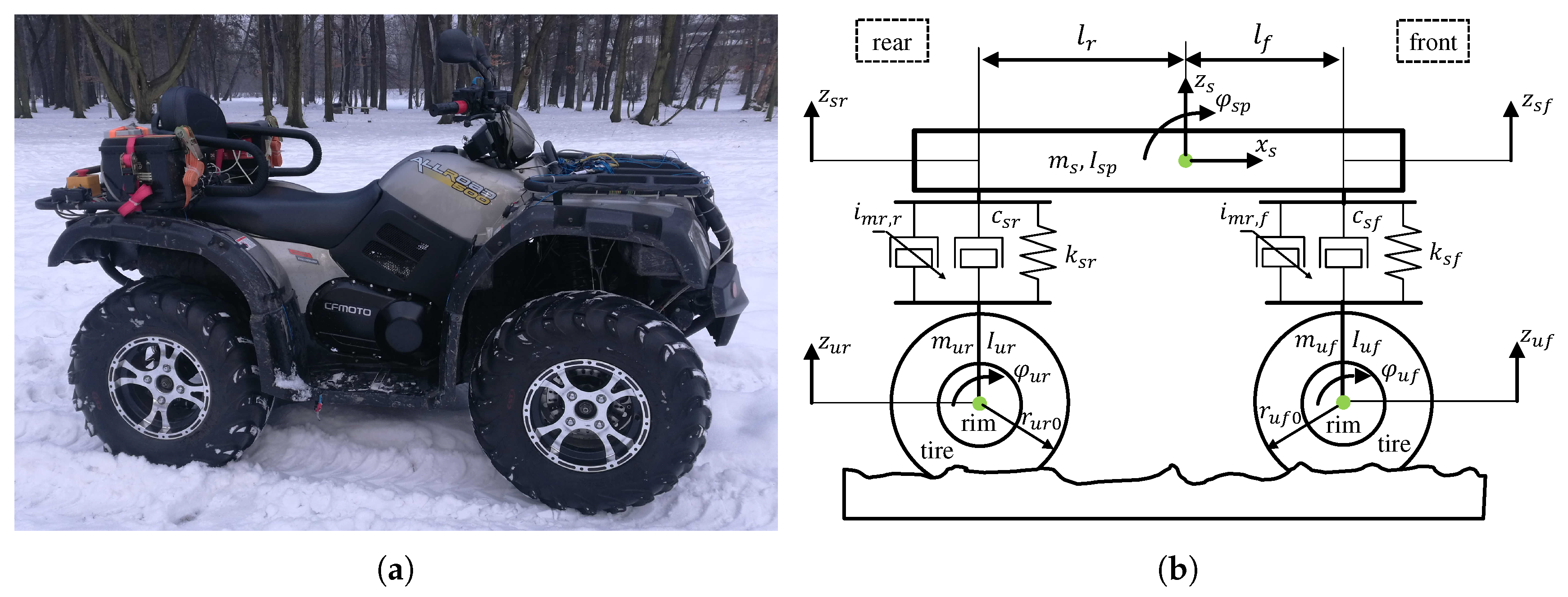
Figure 2.
Standard road profile of class F: (a) with respect to the longitudinal coordinate, (b) spatial power spectral density (PSD) with respect to the spatial frequency.
Figure 2.
Standard road profile of class F: (a) with respect to the longitudinal coordinate, (b) spatial power spectral density (PSD) with respect to the spatial frequency.
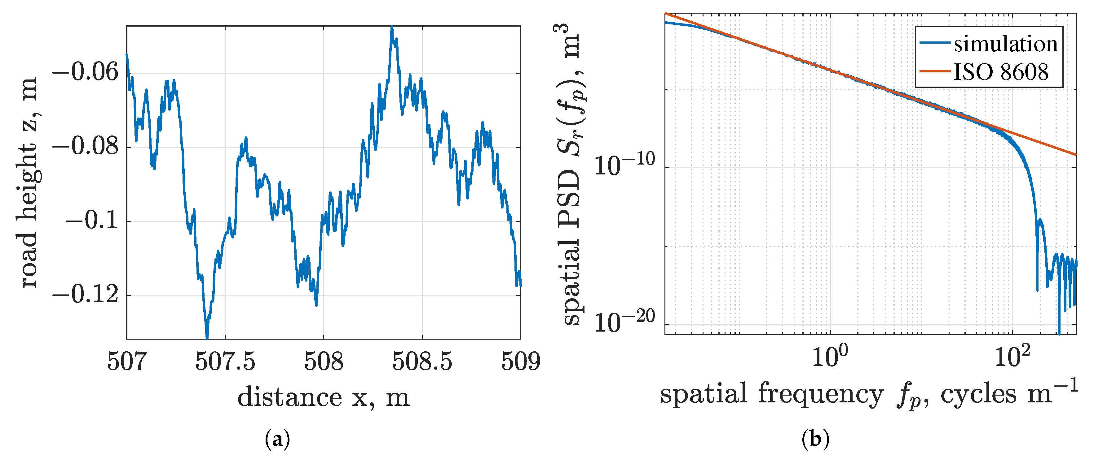
Figure 3.
Tire model for uneven road: (a) tire subjected to road irregularities and ground normal forces, (b) tire stiffness and damping forces.
Figure 3.
Tire model for uneven road: (a) tire subjected to road irregularities and ground normal forces, (b) tire stiffness and damping forces.

Figure 4.
Characteristics of tire to road friction force on slip ratio for the Burckhardt model and wet concrete surface.
Figure 4.
Characteristics of tire to road friction force on slip ratio for the Burckhardt model and wet concrete surface.
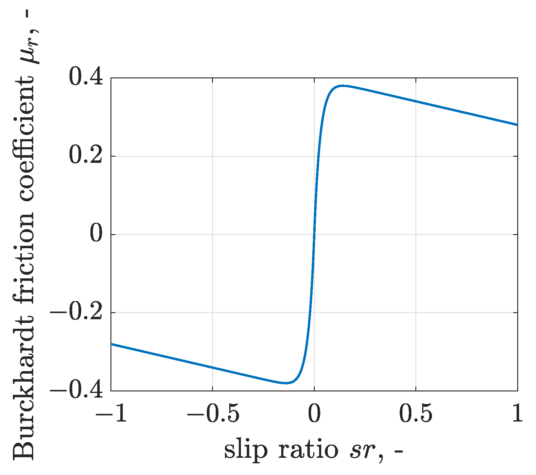
Figure 5.
Force-velocity characteristics of the MR damper based on hyperbolic function.
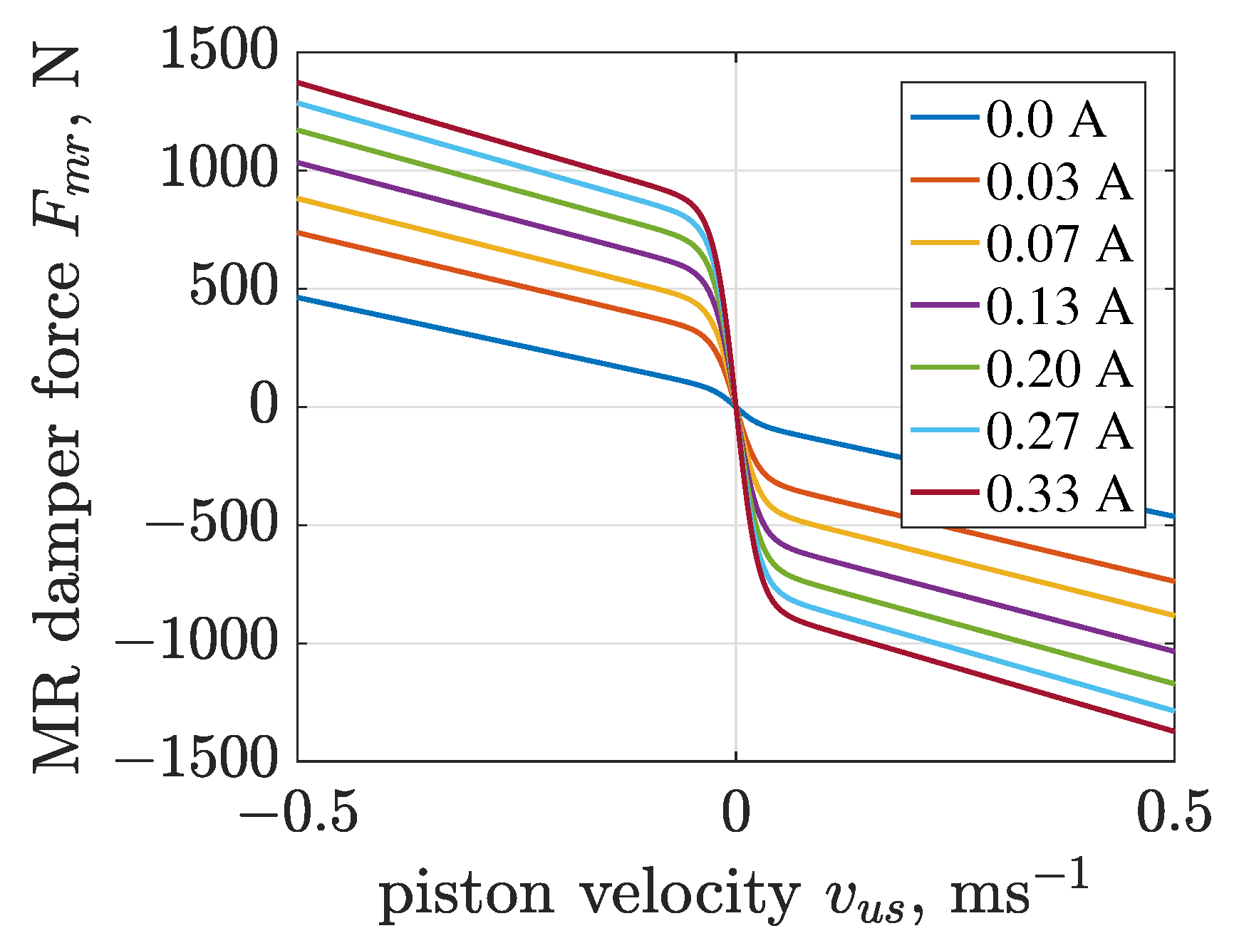
Figure 6.
Block diagram of the control algorithm, including inverse Tanh models.
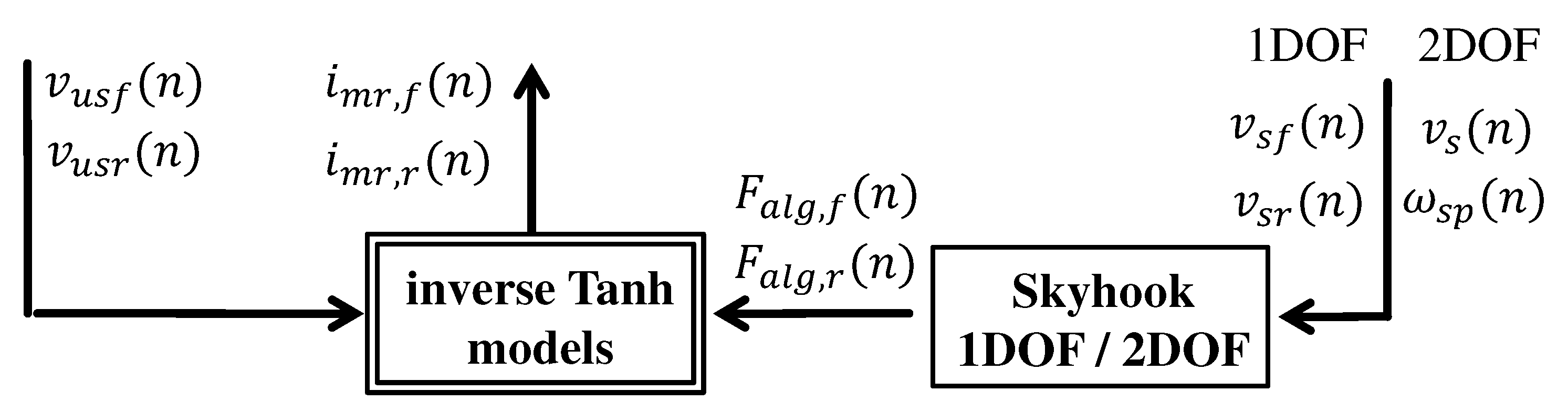
Figure 7.
Block diagram of the simulation environment, section references are given in parentheses. The controller part is presented in Figure 6.
Figure 7.
Block diagram of the simulation environment, section references are given in parentheses. The controller part is presented in Figure 6.
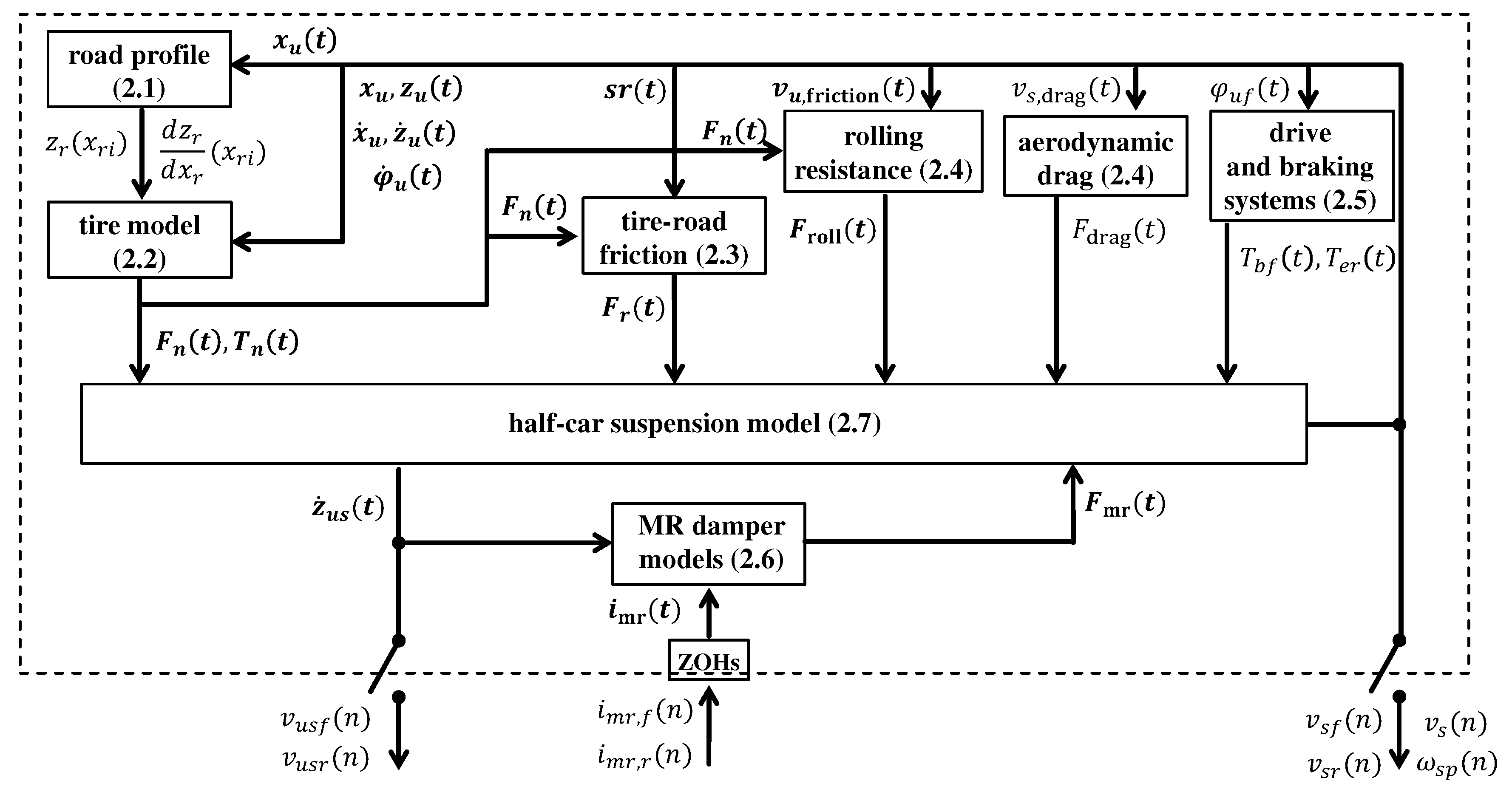
Figure 8.
Procedure of simulation tests of the vehicle model: (a) constant vehicle speed, transmissibilities T, power spectral densities S and values of vehicle handling index were evaluated for simulation data corresponding to the gray area, (b) multiple accelerating and braking phases, the values of road holding index were evaluated for simulation data marked by the following areas: green for accelerating and the rear wheel, red for braking and the front wheel.
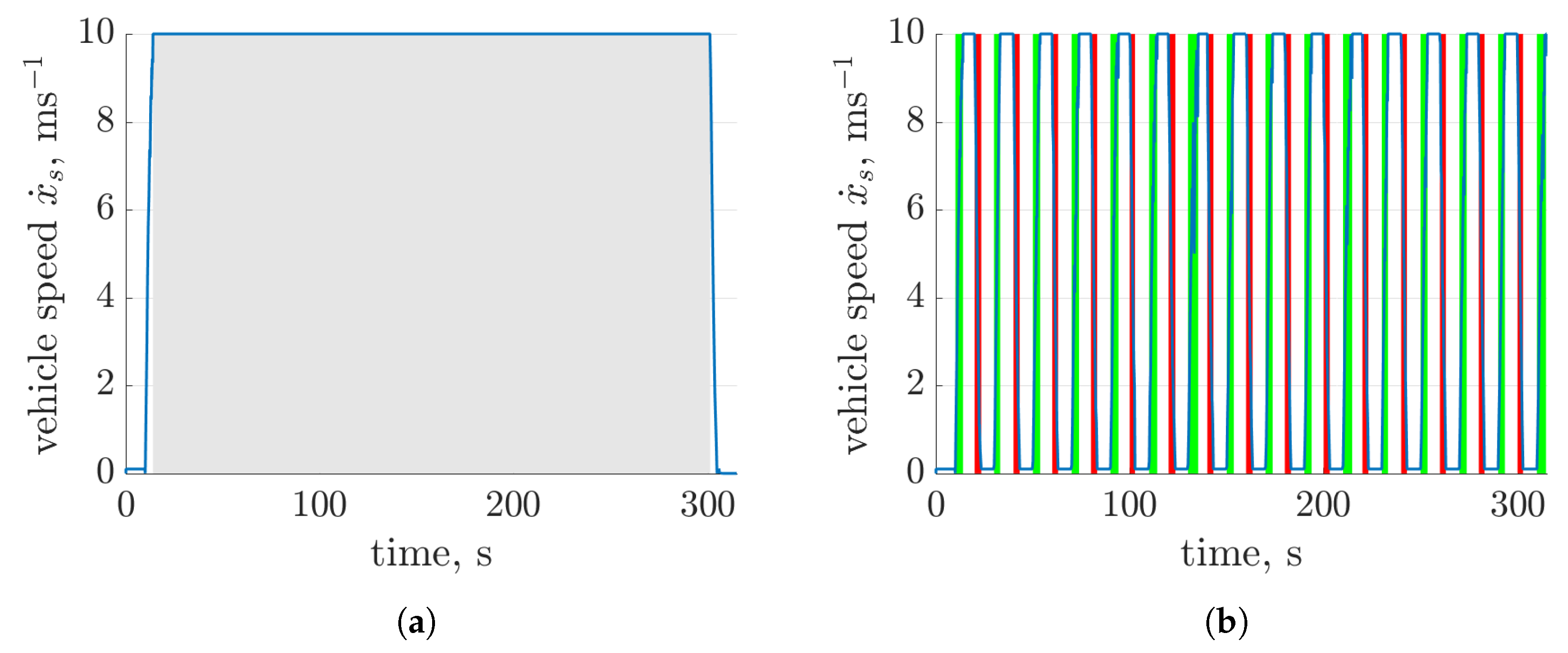
Figure 9.
Time diagrams of slip ratios: (a) front wheel during braking, (b) rear wheel during accelerating.
Figure 9.
Time diagrams of slip ratios: (a) front wheel during braking, (b) rear wheel during accelerating.

Figure 10.
Transmissibility characteristics of vehicle body dynamics for passive suspension and constant vehicle longitudinal velocity equal to 5 ms: (a) heave velocity, (b) pitch velocity.
Figure 10.
Transmissibility characteristics of vehicle body dynamics for passive suspension and constant vehicle longitudinal velocity equal to 5 ms: (a) heave velocity, (b) pitch velocity.
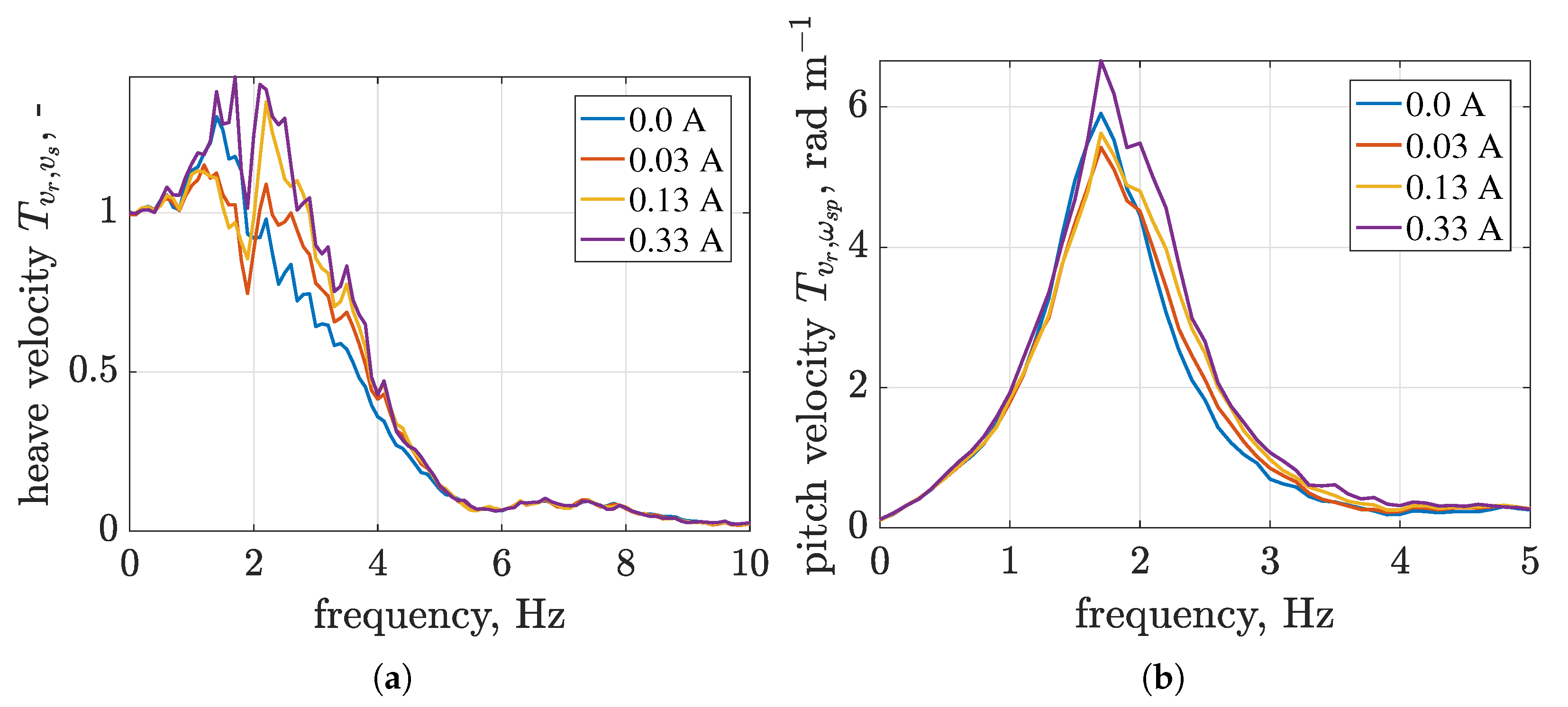
Figure 11.
Transmissibility characteristics of vertical wheel velocity for passive suspension and constant vehicle longitudinal velocity equal to 5 ms: (a) front wheel, (b) rear wheel.
Figure 11.
Transmissibility characteristics of vertical wheel velocity for passive suspension and constant vehicle longitudinal velocity equal to 5 ms: (a) front wheel, (b) rear wheel.
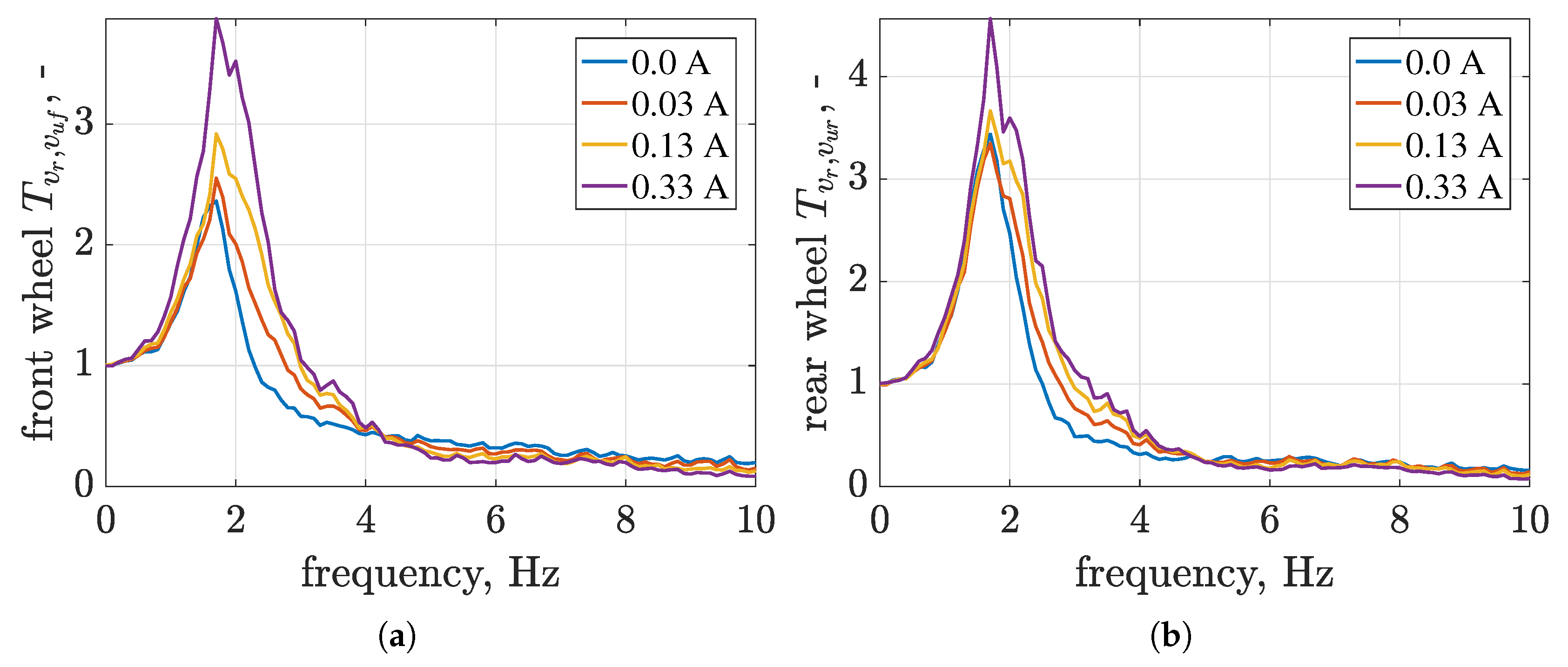
Figure 12.
Power spectral density characteristics of wheel normal forces for passive suspension and the vehicle constant longitudinal velocity 5 ms: (a) front wheel, (b) rear wheel.
Figure 12.
Power spectral density characteristics of wheel normal forces for passive suspension and the vehicle constant longitudinal velocity 5 ms: (a) front wheel, (b) rear wheel.
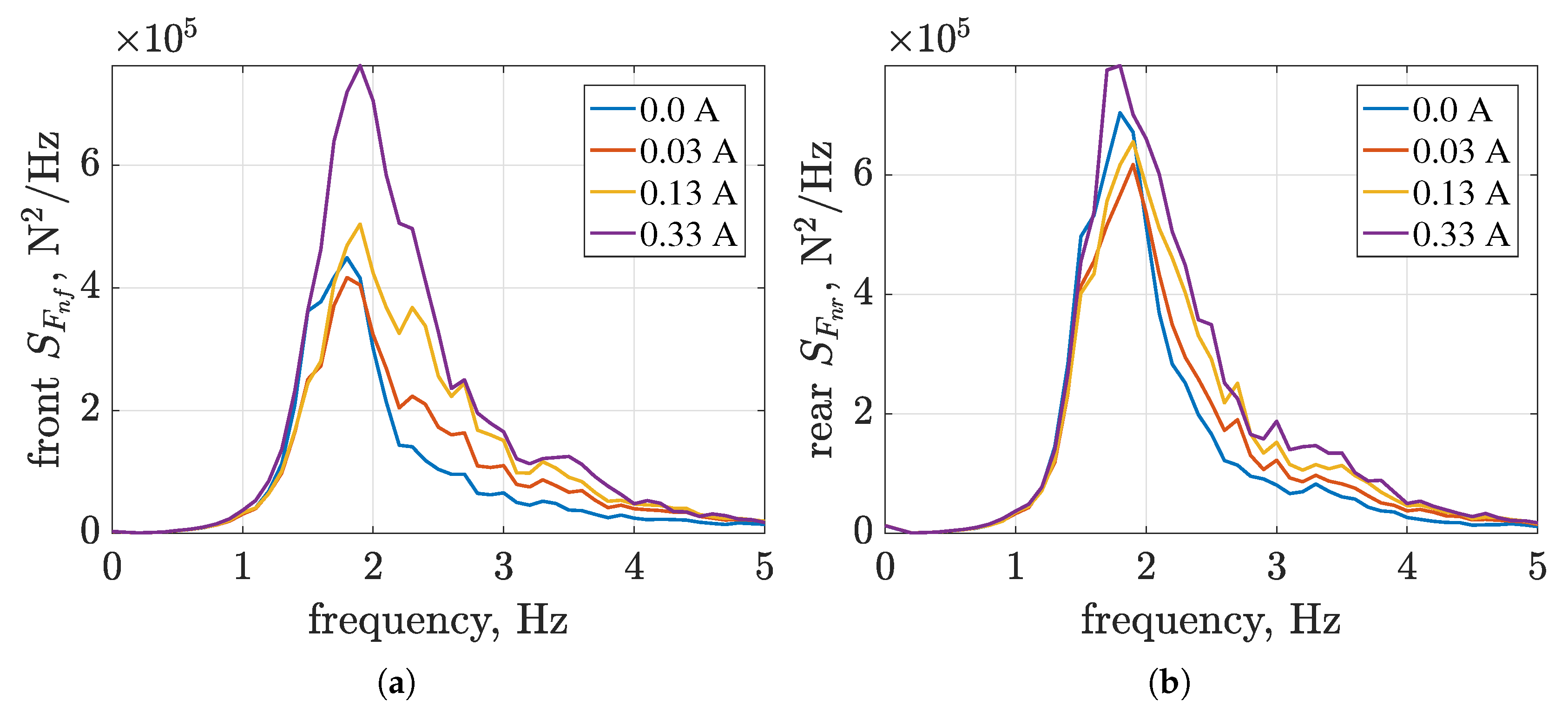
Figure 13.
Transmissibility characteristics of vehicle body dynamics for Skyhook control of suspension parts and vehicle longitudinal velocity equal to 5 ms: (a) front body velocity, (b) rear body velocity.
Figure 13.
Transmissibility characteristics of vehicle body dynamics for Skyhook control of suspension parts and vehicle longitudinal velocity equal to 5 ms: (a) front body velocity, (b) rear body velocity.
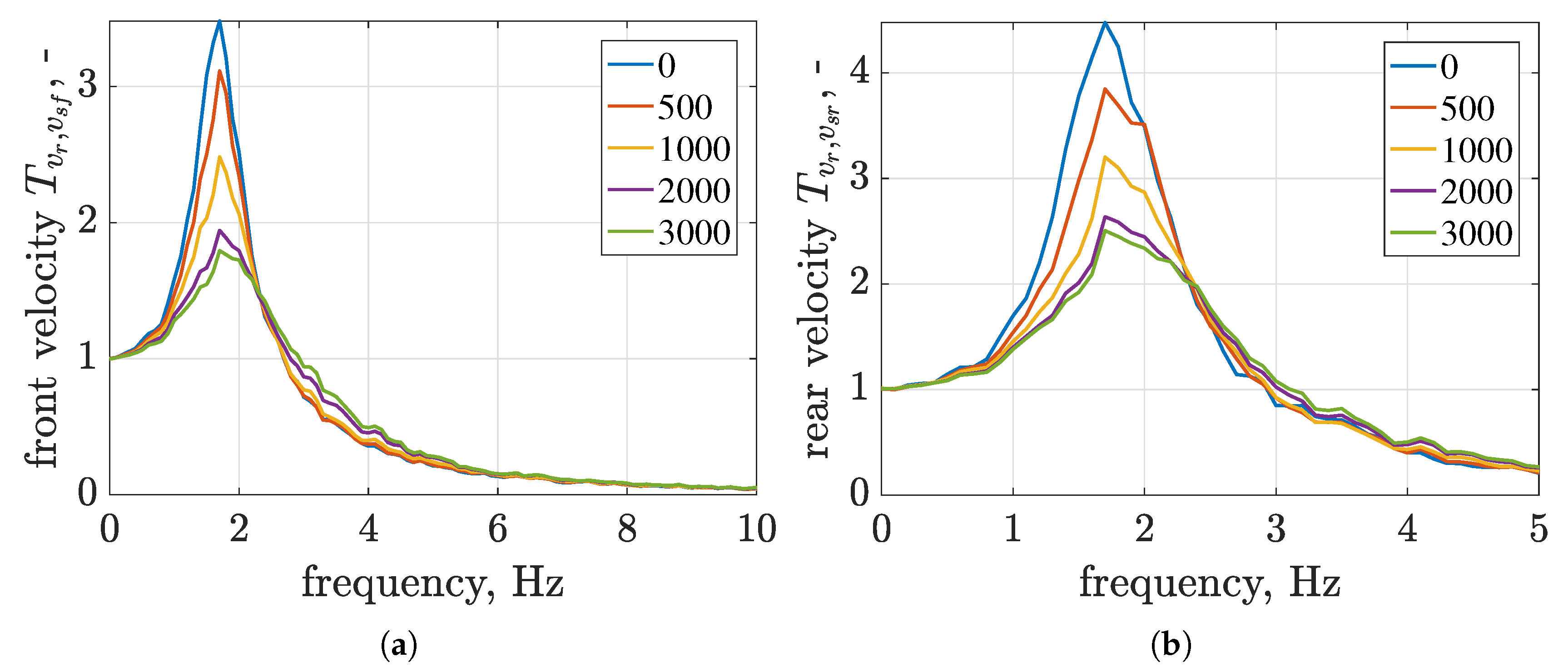
Figure 14.
Power spectral density characteristics of wheel normal forces for Skyhook control of suspension parts (Skyhook-1DOF) and vehicle longitudinal velocity equal to 5 ms: (a) front wheel, (b) rear wheel.
Figure 14.
Power spectral density characteristics of wheel normal forces for Skyhook control of suspension parts (Skyhook-1DOF) and vehicle longitudinal velocity equal to 5 ms: (a) front wheel, (b) rear wheel.
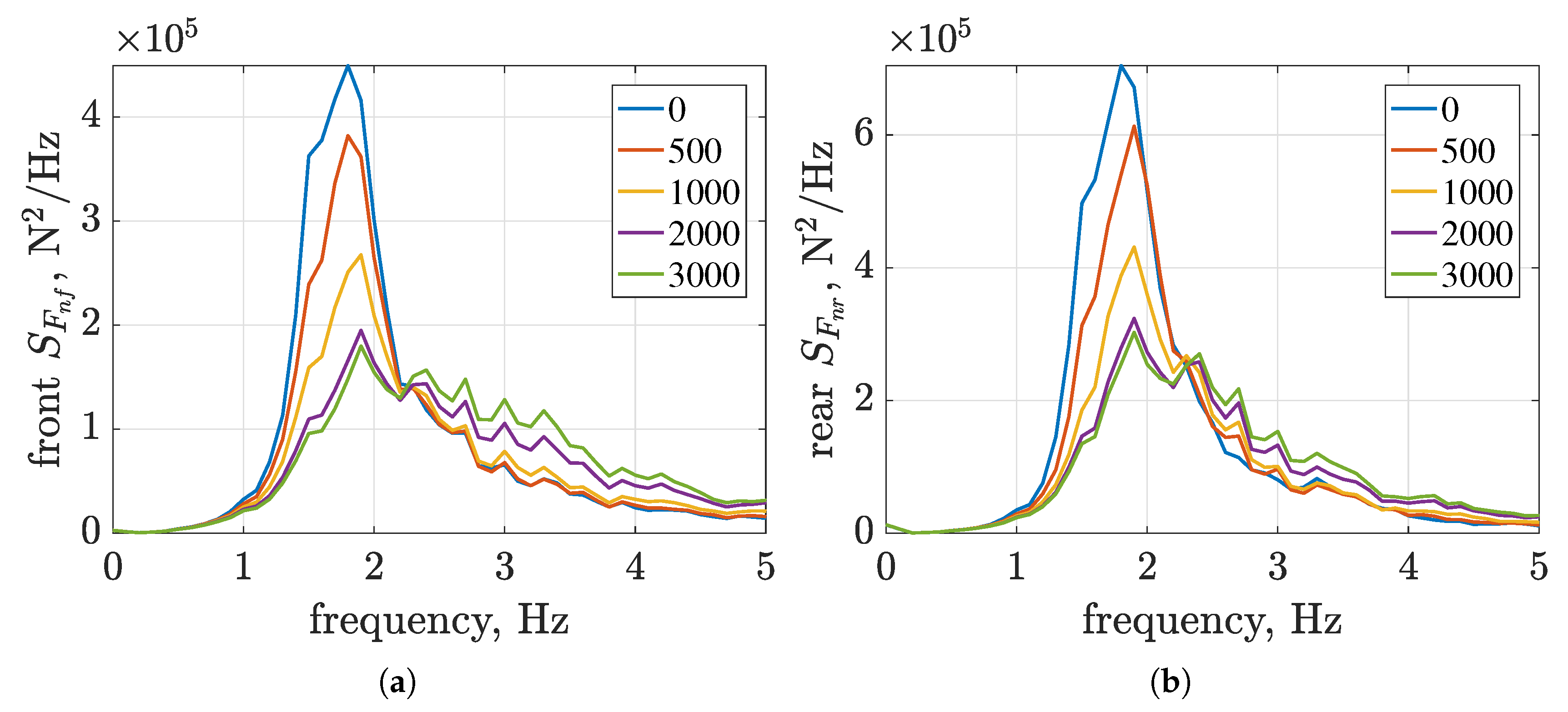
Figure 15.
The transmissibility characteristics of the body dynamics for Skyhook control of the vibration modes (Skyhook-2DOF) at vehicle longitudinal velocity equal to 5 ms: (a) heave velocity, (b) pitch velocity.
Figure 15.
The transmissibility characteristics of the body dynamics for Skyhook control of the vibration modes (Skyhook-2DOF) at vehicle longitudinal velocity equal to 5 ms: (a) heave velocity, (b) pitch velocity.

Figure 16.
Power spectral density characteristics of wheel normal forces for Skyhook control of the body vibration modes (Skyhook-2DOF) and vehicle longitudinal velocity equal to 5 ms: (a) front wheel, (b) rear wheel.
Figure 16.
Power spectral density characteristics of wheel normal forces for Skyhook control of the body vibration modes (Skyhook-2DOF) and vehicle longitudinal velocity equal to 5 ms: (a) front wheel, (b) rear wheel.

Figure 17.
Weighting function dedicated to assessment of tire from road separation for the front and rear wheel.
Figure 17.
Weighting function dedicated to assessment of tire from road separation for the front and rear wheel.
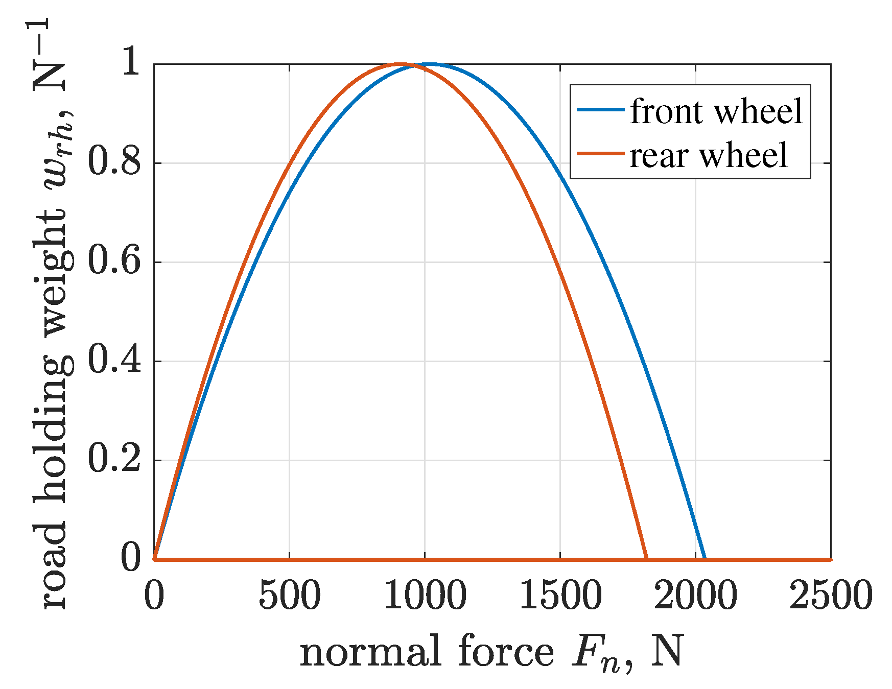
Figure 18.
Comparison of road holding for different suspension settings: passive, separate and coupled Skyhook control for vehicle longitudinal velocity of 5 ms: (a) front wheel during braking, (b) rear wheel during acceleration.
Figure 18.
Comparison of road holding for different suspension settings: passive, separate and coupled Skyhook control for vehicle longitudinal velocity of 5 ms: (a) front wheel during braking, (b) rear wheel during acceleration.
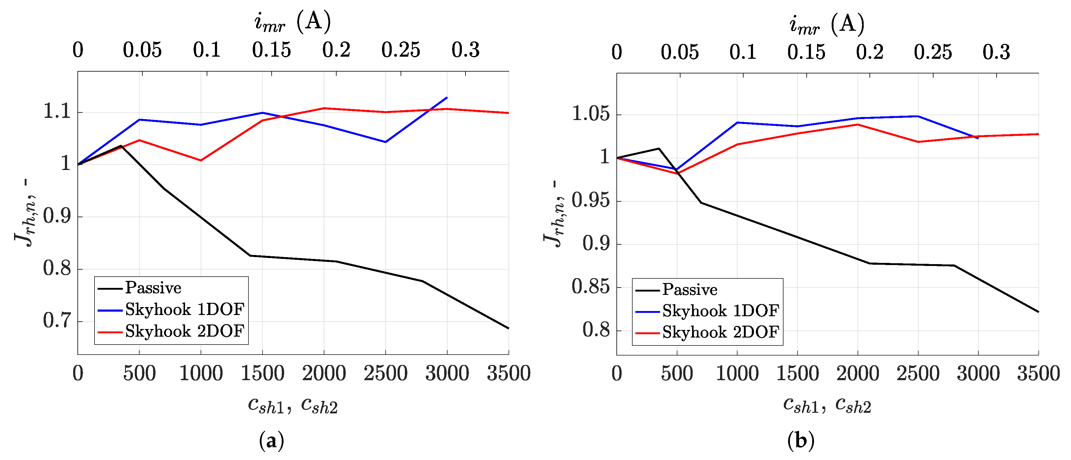
Figure 19.
Comparison of road holding for different suspension settings: passive, separate and coupled Skyhook control for vehicle longitudinal velocity of 10 ms: (a) front wheel during braking, (b) rear wheel during acceleration.
Figure 19.
Comparison of road holding for different suspension settings: passive, separate and coupled Skyhook control for vehicle longitudinal velocity of 10 ms: (a) front wheel during braking, (b) rear wheel during acceleration.
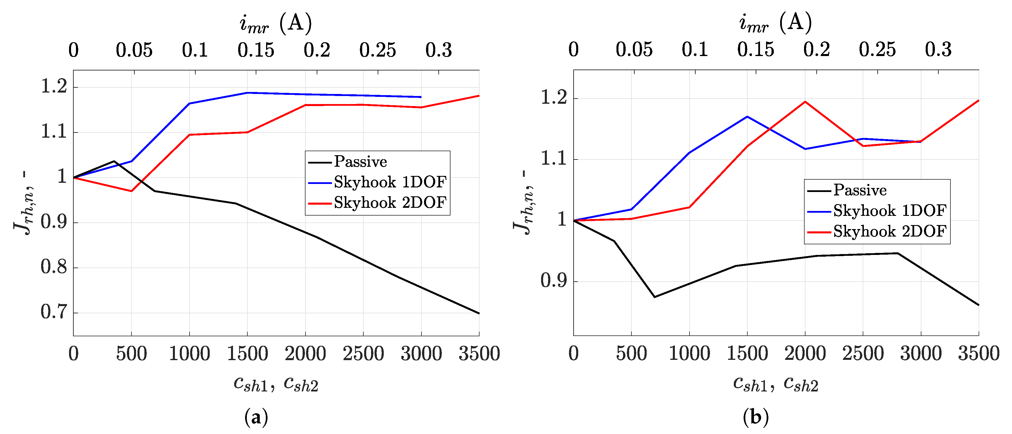
Figure 20.
Comparison of vehicle handling for different suspension settings: passive, separate and coupled Skyhook control: (a) vehicle longitudinal velocity of 5 ms, (b) vehicle longitudinal velocity of 10 ms.
Figure 20.
Comparison of vehicle handling for different suspension settings: passive, separate and coupled Skyhook control: (a) vehicle longitudinal velocity of 5 ms, (b) vehicle longitudinal velocity of 10 ms.


Table 1.
Parameters of the vehicle model and its submodels.
| Road profile and simulation parameters | |||||||||||
| = 1000 Hz | = 1000 points m | rc (road class) = F | = 6.6 m | ||||||||
| 4 DoFs half-car suspension model | |||||||||||
| = 171.5 kg | = 74.3 kgm | ||||||||||
| = 0.609 m | = 0.681 m | = 0.554 m | |||||||||
| = 22.208 kNm | = 34.857 kNm | = 300 Nsm | = 300 Nsm | ||||||||
| based model of the MR damper | |||||||||||
| (0.0; 1.33) A | = 62.42 N | = 1340 N | |||||||||
| = 39.96 sm | = 802.8 Nsm | = 488.5 Nsm | |||||||||
| Wheel and tire models | |||||||||||
| = 10 kg | = 15 kg | = 0.6 kgm | = 0.9 kgm | ||||||||
| = 0.317 m | = 0.317 m | = 0.244 m | = 0.244 m | ||||||||
| = 5234.1 Nm | = 5113.6 Nm | = 447.3 Nsm | = 560.4 Nsm | ||||||||
| Burckhardt model of tire to road friction for wet concrete surface | |||||||||||
| = 0.4004 | = 33.7080 | = 0.1204 | |||||||||
| Rolling resistance for concrete surface and aerodynamic drag | |||||||||||
| = 0.008 | |||||||||||
| = 1.223 kgm | = 0.72 | = 1.75 m | |||||||||
| Parameters of front braking and rear drive systems for half-car model | |||||||||||
| = 160 Nm | = 225 Nm | ||||||||||
Publisher’s Note: MDPI stays neutral with regard to jurisdictional claims in published maps and institutional affiliations. |
© 2020 by the authors. Licensee MDPI, Basel, Switzerland. This article is an open access article distributed under the terms and conditions of the Creative Commons Attribution (CC BY) license (http://creativecommons.org/licenses/by/4.0/).
Share and Cite
MDPI and ACS Style
Krauze, P.; Kasprzyk, J. Driving Safety Improved with Control of Magnetorheological Dampers in Vehicle Suspension. Appl. Sci. 2020, 10, 8892. https://doi.org/10.3390/app10248892
AMA Style
Krauze P, Kasprzyk J. Driving Safety Improved with Control of Magnetorheological Dampers in Vehicle Suspension. Applied Sciences. 2020; 10(24):8892. https://doi.org/10.3390/app10248892
Chicago/Turabian StyleKrauze, Piotr, and Jerzy Kasprzyk. 2020. "Driving Safety Improved with Control of Magnetorheological Dampers in Vehicle Suspension" Applied Sciences 10, no. 24: 8892. https://doi.org/10.3390/app10248892
Note that from the first issue of 2016, this journal uses article numbers instead of page numbers. See further details here.