Article

Solar Cell Cracks and Finger Failure Detection Using Statistical Parameters of Electroluminescence Images and Machine Learning

1
Department of Energy Technology, AAU, 9220 Aalborg, Denmark
2
School of Photovoltaic and Renewable Energy Engineering, UNSW, Kensington, NSW 2052, Australia
3
Department of Photonics Engineering, Technical University of Denmark, 4000 Roskilde, Denmark
4
PI Photovoltaik-Institut Berlin AG, Wrangelstr. 100, D-10997 Berlin, Germany
5
School of Electrical Engineering and Robotics, Queensland University of Technology, Brisbane, QLD 4000, Australia
*
Author to whom correspondence should be addressed.
Appl. Sci. 2020, 10(24), 8834; https://doi.org/10.3390/app10248834
Submission received: 27 October 2020 / Revised: 7 December 2020 / Accepted: 8 December 2020 / Published: 10 December 2020
(This article belongs to the Special Issue Fault Diagnosis and Control Design Applications of Energy Systems)

Abstract

:
A wide range of defects, failures, and degradation can develop at different stages in the lifetime of photovoltaic modules. To accurately assess their effect on the module performance, these failures need to be quantified. Electroluminescence (EL) imaging is a powerful diagnostic method, providing high spatial resolution images of solar cells and modules. EL images allow the identification and quantification of different types of failures, including those in high recombination regions, as well as series resistance-related problems. In this study, almost 46,000 EL cell images are extracted from photovoltaic modules with different defects. We present a method that extracts statistical parameters from the histogram of these images and utilizes them as a feature descriptor. Machine learning algorithms are then trained using this descriptor to classify the detected defects into three categories: (i) cracks (Mode B and C), (ii) micro-cracks (Mode A) and finger failures, and (iii) no failures. By comparing the developed methods with the commonly used one, this study demonstrates that the pre-processing of images into a feature vector of statistical parameters provides a higher classification accuracy than would be obtained by raw images alone. The proposed method can autonomously detect cracks and finger failures, enabling outdoor EL inspection using a drone-mounted system for quick assessments of photovoltaic fields.

1. Introduction

With the significant increase in the necessity of photovoltaic (PV) energy generation to curb climate change, the installation of large PV plants has grown significantly in the last decade [1]. As it is desirable to operate these plants at their maximum capacity, monitoring the performance of the installed PV modules is critical [2].
Cracks in solar cells have received significant attention in the last years [3]. Cracks are often classified into three modes: micro-cracks (Mode A) and cracks (Mode B and C) [4]. Generally, a micro-crack Mode A does not have a significant impact on the output power. The loss due to the impacted cell area is relatively low, as long as the different regions are electrically connected [4]. However, cracks (Mode B and C) do affect the power output of the PV module. Cells with Mode B cracks exhibit an increase in resistance and lower voltage in the cracked regions [5], while cells with Mode C form a wholly isolated and electrically disconnected cell area. In some cases, cracks (Mode B and C) lead to reverse biasing of the solar cell [6]. In others, 16–25% of the cell area can be separated by cracks parallel to the busbars [7]. The cracks can form due to mechanical stress during transportation or manufacturing installation and maintenance of the modules [7]. A brief classification of the different crack modes is provided in Reference [8].
Another common extrinsic fault type is finger interruptions, usually induced during cell metallization and module interconnection. Finger breaks often result in increased series resistance and, consequently, decreased output power [9,10].
Electroluminescence (EL) imaging has become an indispensable tool for distinguishing various types of failures and different degradation mechanisms with high resolution [11]. EL imaging is based on biasing the modules and measuring the emitted emission, which correlates with the radiative recombination of carriers within the device [12]. As the local luminescence intensity is related to the carrier concentration, faulty and disconnected regions appear darker, depending on the severity of the fault. EL imaging has been used to detect a wide range of defects, such as micro-cracks and cracks, finger interruptions, ribbon damage, and many more [3]. EL imaging can also quantify power losses and the percentage of disconnected regions due to the gap between cell parts and cracks by modifying the bias current [6,13]. Analyzing EL images is typically time-consuming [14] and requires expert knowledge regarding the different defects. It is, therefore, expensive to perform on a large scale [15]. One possible path to improve the analysis is using machine learning (ML) to detect different defects more accurately. A recent advancement has meant outdoor PL images could be obtained by switching the operating module condition through modulating the shading on three cells connected to three different bypass diodes using a high-power light-emitting diode (LED) array. PL has an additional benefit over EL, as it is a contactless technique, and therefore does not require a qualified electrician to change any wiring of the inspected PV system [16].
ML uses predictive or descriptive algorithms to optimize a performance model using a given dataset [17]. The models are built based on the available data to make predictions without being explicitly programmed to perform the task [18]. This study investigates the use of machine learning (ML) to classify the defects mentioned above.
Recently, different ML algorithms have been used to classify various degradation types in EL images. Fada et al. used a supervised ML algorithm to classify a database of 14,200 images into three labels: good, busbar corrosion, and cracked [15]. They used three ML algorithms [support vector machine (SVM), random forest (RF), and multilayer perceptron-artificial neural network (MLP-ANN)] and compared their performance. The cracked cells’ classification accuracy was relatively low, especially compared to the good and corroded groups, possibly due to the unbalanced dataset (as most cells did not have any fault). Karimi et al., who manually categorized the database into four labels: good, cracked, cell edge darkening, and heavily busbar corroded, later extended their study in Reference [19]. They used an unsupervised clustering technique to correlate intrinsic patterns in the images with the supervised labels. The method is based on binary classification (‘degraded’ and ‘non-degraded’ cells), achieving a mean accuracy of 98.9% and 98.2% for SVM and convolutional neural network (CNN) ML algorithms. Additionally, several automated fault detection methods have been proposed [20,21,22]. Sun et al., achieved an overall prediction accuracy of 98.4% using 2000 training steps (25 epochs) [20], while Tseng et al., employed a binary clustering of features to detect only finger interruptions. However, it seems challenging to detect defects with more elaborate structures due to shape assumptions [21]. SVM and RF classifiers were evaluated in Reference [22] using two cell region extraction algorithms. The study focused on the cracked and faulty region’s geometry to distinguish it from a healthy area. Another approach that integrates mini-batch k-means with state-of-the-art clustering CNN has been proposed [23]. The method uses a feature drift compensation to reduce errors caused by a feature mismatch. The technique demonstrates a high accuracy and can efficiently compute millions of images, outperforming existing state-of-art clustering methods [14]. A different approach that uses an independent component analysis (ICA) has been demonstrated to achieve a 93.4% accuracy with a relatively small training dataset of only 300 solar cell images [24]. However, material defects such as finger interruptions are treated equally to cell cracks. Moreover, an algorithm using anisotropic diffusion filtering to locate micro-cracks in polycrystalline solar cells is described in Reference [25]. The method precisely detected the micro-cracks with an accuracy and sensitivity of 88% and 97%, respectively.
Recently, deep learning-based approaches have been suggested for classification [26,27,28,29,30]. A pre-trained visual geometry group (Vgg)-16 CNN network architecture combined with an SVM decision layer was used to classify different faults, achieving 90.2% accuracy [26]. The work was later extended in Reference [27] by developing an enhanced CNN model proposing an algorithmic solution, which extensively evaluated the model performance using different inputs (dataset sizes, learned features, conventional solution, and more). The study demonstrated efficient defect detection of faults, achieving a mean accuracy of 97.9%. A transfer learning-based solution was proposed by Ding et al. [28], which can identify visible defects in large-scale PV plants and distributed rooftop systems. The study uses an enhanced CNN-based model for classification, reaching a 98.9% mean accuracy. A visual defect detection method based on multi-spectral deep CNN has also been proposed [29], achieving an overall defect-recognition accuracy of 94.3%. The effectiveness of a data augmented method, auxiliary classifier-progressive growing generative adversarial networks, was evaluated using three selected CNN models [30]. It has been shown to improve the classification accuracy maximum by 14% in the material defect category compared to a more traditional data augmentation approach.
In this study, we use extracted statistical parameters from the image histogram as a feature descriptor. The vector is then fed into different ML classifiers to distinguish between various defects. We demonstrate that processing the images into a feature vector of statistical parameters has a significant advantage over the standard methods that use many features.

2. Methodology

In this study, 753 EL images of multi-crystalline silicon (mc-Si) aluminum and back surface (Al-BSF) modules are used (~46,000 cell images). The modules are from different PV arrays installed in various locations across the United Kingdom (Oxford-shire, Norfolk, Hampshire, and Somerset).
The EL images were acquired using a modified complementary metal-oxide-semiconductor (CMOS) camera (Nikon D750) that was modified by replacing the embedded infrared filter with a daylight filter (850–1700 nm). The images were acquired outdoors one hour before sunset, at approximately 17:00 (during August–September 2016), with a tripod holding the camera perpendicular to the module at a distance of 2–3 m. The exposure time ranged between 5 and 10 s, while the bias current was fixed at 5A.
Two experts in EL-based PV diagnostics then classified the cell images into three classes: (i) cracks (Mode B and C), (ii) finger failures and micro-cracks (Mode A), and (iii) no failures. Examples of the three different classes are presented in Figure 1. Finger failures and micro-cracks (Mode A), cracks (Mode B and C) are combined since the failures look similar in terms of structure, length, and intensity. More importantly, they have a similar effect on the module’s output power. Cells that contain more than one type of fault are labeled according to the more severe defect (i) > (ii) > (iii). The following image processing and machine learning part will be discussed in the section below.

2.1. Image Processing

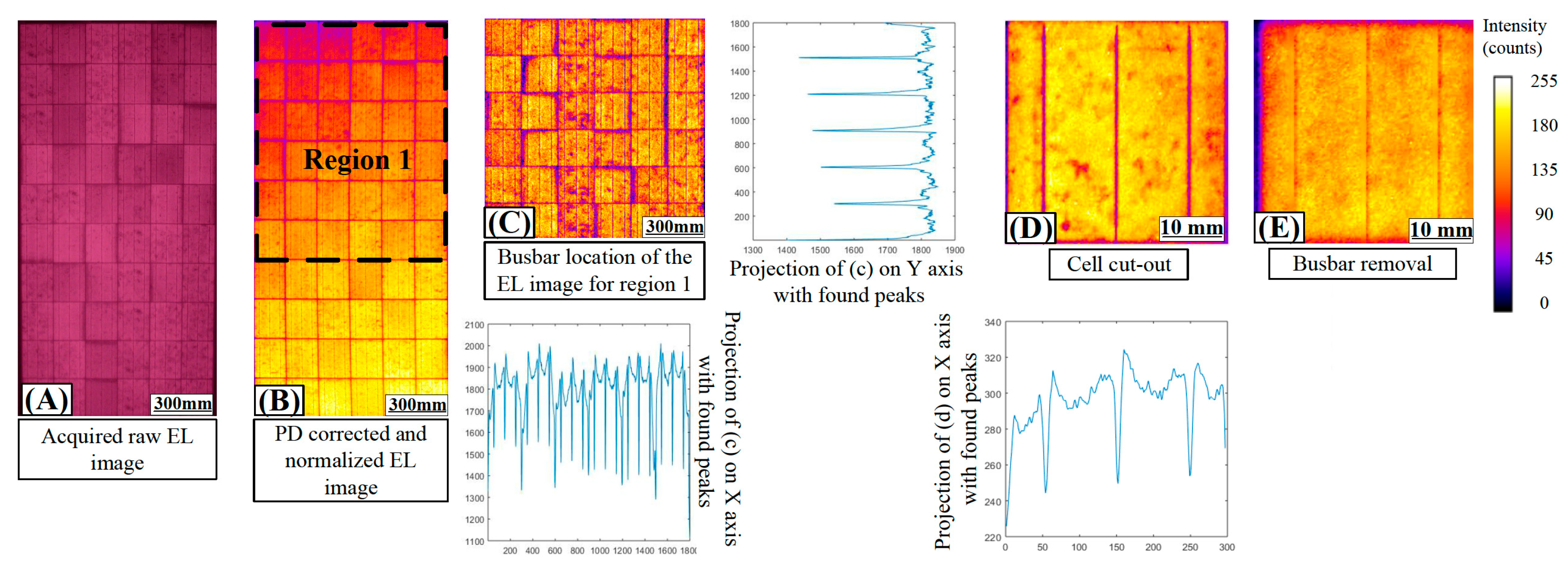
Before being used as an input for ML, the images need to be processed to correct several effects. The correction processes are summarized in Figure 2 and discussed below.
Firstly, despite the effort to keep the camera in the same position compared to the module, variations always occur, especially when considering the measurement conditions (outdoor, evening, possible wind). Furthermore, as the images are taken at an angle, they are distorted. Hence, the first step is to correct the images for the perspective distortion [31,32,33] using a code developed in Matlab [34]. The active module area is aligned, and the perspective is fixed following the procedure of Reference [35], as shown in Figure 2B. The cell images are then resized from 300 × 300 to 100 × 100 pixels to reduce computation time. They are then normalized using min-max scaling features to standardize the dataset for systematic analysis. Blurred images are identified using blur detection based on the modified Laplacian matrix technique described in Reference [36].
An appropriate threshold value (0.80) is chosen, and EL images below this threshold are defined as ‘blurred’ and discarded. The module images are then segmented into cells [37]. The module and cell edges are computed by rotating the processed image at different angles and summing the pixel values along the x and y axes to locate the horizontal and vertical lines, as shown in Figure 2C. If distortion is identified, the images are perspective-corrected, using homography transformation [31,32]. Note that this is a second distortion correction for the case where the correction on the module level is not sufficient. Busbars are then removed from the cell images by first locating them (similar method to identifying the edges) and then adjusting pixel values to the neighboring pixels’ mean, as shown in Figure 2E.

2.2. Machine Learning Classifiers

Three supervised ML algorithms (SVM, RF, and k-NN) are trained and compared using the feature vectors (see below) and target labels [38,39]. The code was written using Python with its additional packages of NumPy, Pandas, sklearn, SciPy, and matplotlib [40,41]. The code can be shared on GitHub upon request. However, the authors would not be able to share the PI-Berlin dataset as it is not public.
Support Vector Machine: SVM’s core idea is finding a decision boundary (hyper-plane) that helps separate space vector/dataset into classes. The decision boundary is searched through the maximum margin classifier, which is decided by the support vectors. SVM generates an optimal hyperplane in an iterative manner, which is used to minimize errors. The distance between the nearest points is known as the margin. The hyper-plane is selected based on the maximum possible margin between support vectors [17,42]. A radial basis function (RBF) is used as a kernel function in this study, and other hyper-parameters like (penalty parameter ‘C’, gamma) are found by implementing a grid search to find the optimal value [43].
Random Forest: RF is an ensemble of ML techniques that builds multiple decision tree classifiers on random sub-samples of the training dataset. Each decision tree predicts the response by following the tree’s decisions from the root to the leaf. The output of each decision tree is then averaged to determine the prediction [44]. RF’s main advantage is leveraging the power of a large number of randomly selected trees to represent the solution. Thus, instead of using one decision tree, RF uses all the decision trees to determine the classification; this procedure reduces errors and uncertainties [42]. In this study, the number of trees selected was 5 and 10. The minimum number of samples that are required to split an internal node is set to 25. The maximum depth of the tree is kept at five [45].
k-Nearest Neighbors: k-NN categorizes objects based on their nearest neighbors’ classes in the dataset, assuming the neighbor objects are similar. This non-parametric method does not make any assumptions regarding the underlying data distribution. Instead, it chooses to memorize the training instances used in the supervised training. This method’s main limitation is its intensive time and memory requirements [17,39]. In this study, parameters are selected by implementing a grid search regarding neighbors [46].

3. Implemented Feature Vectors and Data Labelling

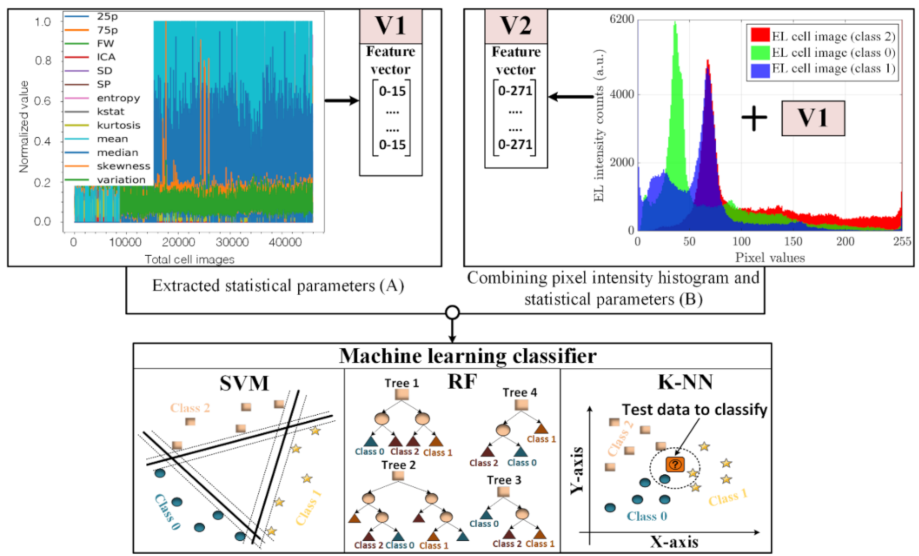
Figure 3 presents the procedure used in this study. This study’s focus is on the selection of the feature vector (gray box in the diagram). The EL intensity of each of the pixels is used to determine the intensity distribution across the image. Different derived statistical parameters are then calculated based on the 1D pixel intensity histogram of high-resolution images (see Table A1). The proposed feature vector V1 contains 16 statistical parameters reducing the feature vector’s dimension by encoding the information into a smaller latent space to remove the redundant information from the data. This allows an efficient and fast process compared to the traditional methods, which use the 2D spatial information to identify the image’s defects. Finally, the developed feature vectors (V1 and V2) are used as an input for the three ML classifiers, as shown in Figure 4, for classifying the defects in the images.
As discussed, the defects are classified into three classes: (i) cracks (Mode B and C) (Class 0), (ii) finger failures and micro-cracks Mode A (Class 1), and (iii) no failures (Class 2). In total, 1385 defects have been identified (see Table 1).
Statistical output metrics [47] such as recall, precision, accuracy, and F1 score are defined and used to evaluate the algorithms [47] (see definitions in Table 2).
The recall metric measures the percentage of total relevant results correctly classified by the algorithm, while precision is the ratio between correctly labeled positive outcomes and the total predicted positive outcomes. Accuracy is defined as the strength of the correlation between the predicted and the actual labels [47]. It is given as the ratio between the number of correct predictions and the total number of predictions. Nevertheless, accuracy is not the best representation of performance on unbalanced datasets. Hence, the F1 score metric, defined as the harmonic mean of precision and recall, is also computed in this study. It has been shown that the F1 score is a better indicator when analyzing unbalanced datasets [47].
For the training stage, to prevent under-fitting or over-fitting, Class 2 (no failures) is downsampled to 2185 cell images with approximately 700 cell images of each class label (as shown in Table 1). The training is done on 75% of the dataset, while the remaining 25% is used to evaluate the algorithm on previously unseen data (validation dataset) [48].

4. Results and Performance Discussion

Performance Analysis

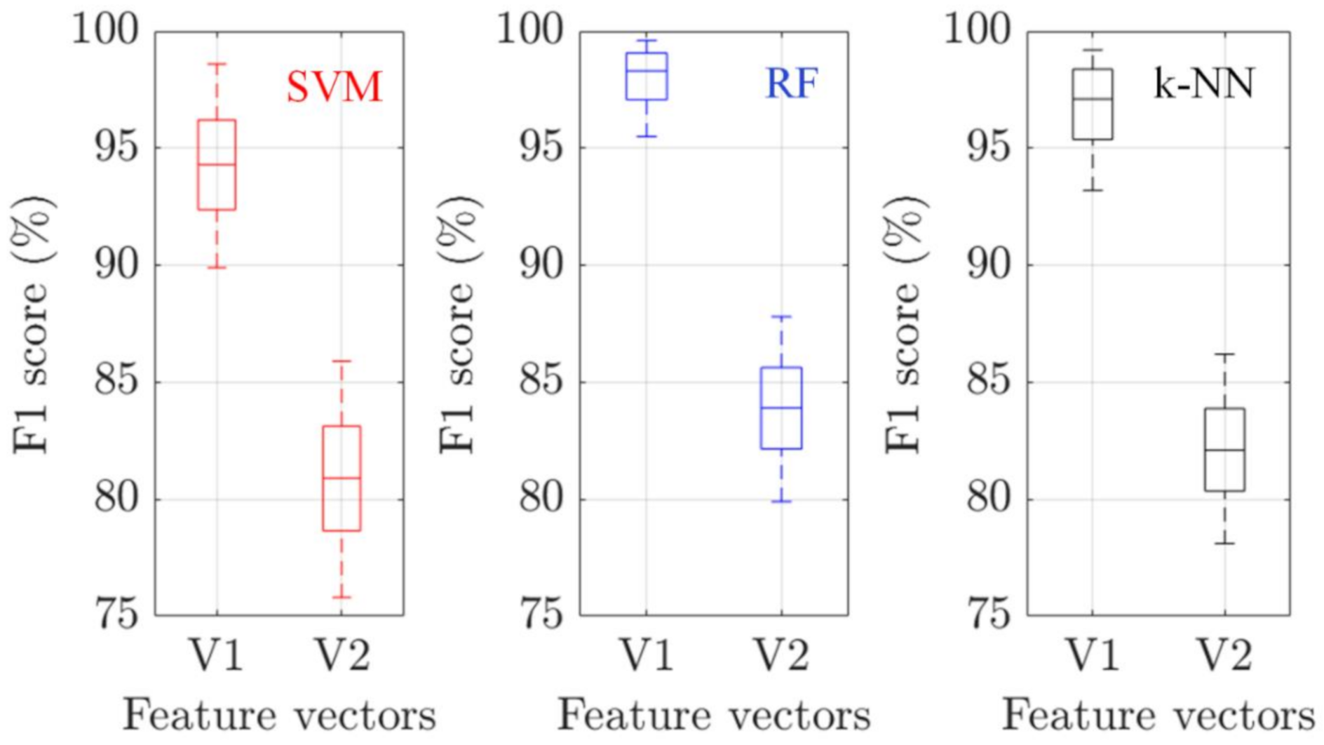
Figure 5 compares the F1 scores of the two feature vectors when they are used as inputs to the three ML classifiers (SVM, RF, and k-NN) of the validation set. The validation has been repeated five times to extract statistical parameters. In all cases, the proposed vector (V1) outperforms the combined approach (V2), achieving higher F1 scores with lower variance. Hence, it can be concluded that the larger number of pixel intensity features in the case of V2 (256) masks the unique features (16) that are used by V1, substantially reducing the performance of the ML classifiers. No significant difference can be observed between different ML algorithms. Note that a comparison between the training and validation sets indicates that the data has not been over-fitted.
Table 3 summarizes the two vectors’ performance using the other output metrics: accuracy, recall, and precision. As can be seen, V1 performs better across all categories. We note that V1 as a feature vector and RF as a classifier is the best combination for performance evaluation, achieving 99.6% accuracy.
Table 4 compares the F1 scores obtained in this study and scores reported in the literature for thorough analysis. The obtained F1 scores of V1 are higher than the scores reported for the isolated in-depth training and transfer learning approaches [8,14]. They are also higher than those obtained by the Kaze/VGG feature vector combined with an SVM classifier and spectral clustering algorithm [14,21]. It is noticeable that our scores are similar to the best-reported scores, despite the relatively small dataset (2185 images) and without data augmentation. Moreover, the proposed method requires less computational time in terms of feature extraction and training time because the feature vector’s size is curtailed to 16 from 256 (standard).
Table 4 also summarizes the reported accuracies. This study’s obtained accuracy is similar to the highest reported accuracy that uses a two-image region/area detection algorithm for classification [22]. Despite the high overall precision, the two-region algorithm for EL cell images achieved a low F1 score (5.1%) and recall (27.4%) values, probably due to an unbalanced dataset. The output metric results can be improved by calculating the geometric mean for unbalanced class sizes. Moreover, this study’s obtained accuracy is higher than recorded in Reference [15], which compares the supervised classifiers (SVM and RF) with CNN using the stochastic gradient descent method. They achieved the overall best accuracy, 98.77%, with the least computation time of (85.52 s) using the SVM classifier compared to 98.13% accuracy with (2250 s) of computation time using the CNN method. Moreover, Reference [19] recorded 98% accuracy computing Haralicks features as a feature vector for detecting different failures using an SVM classifier, as mentioned in Table 4.
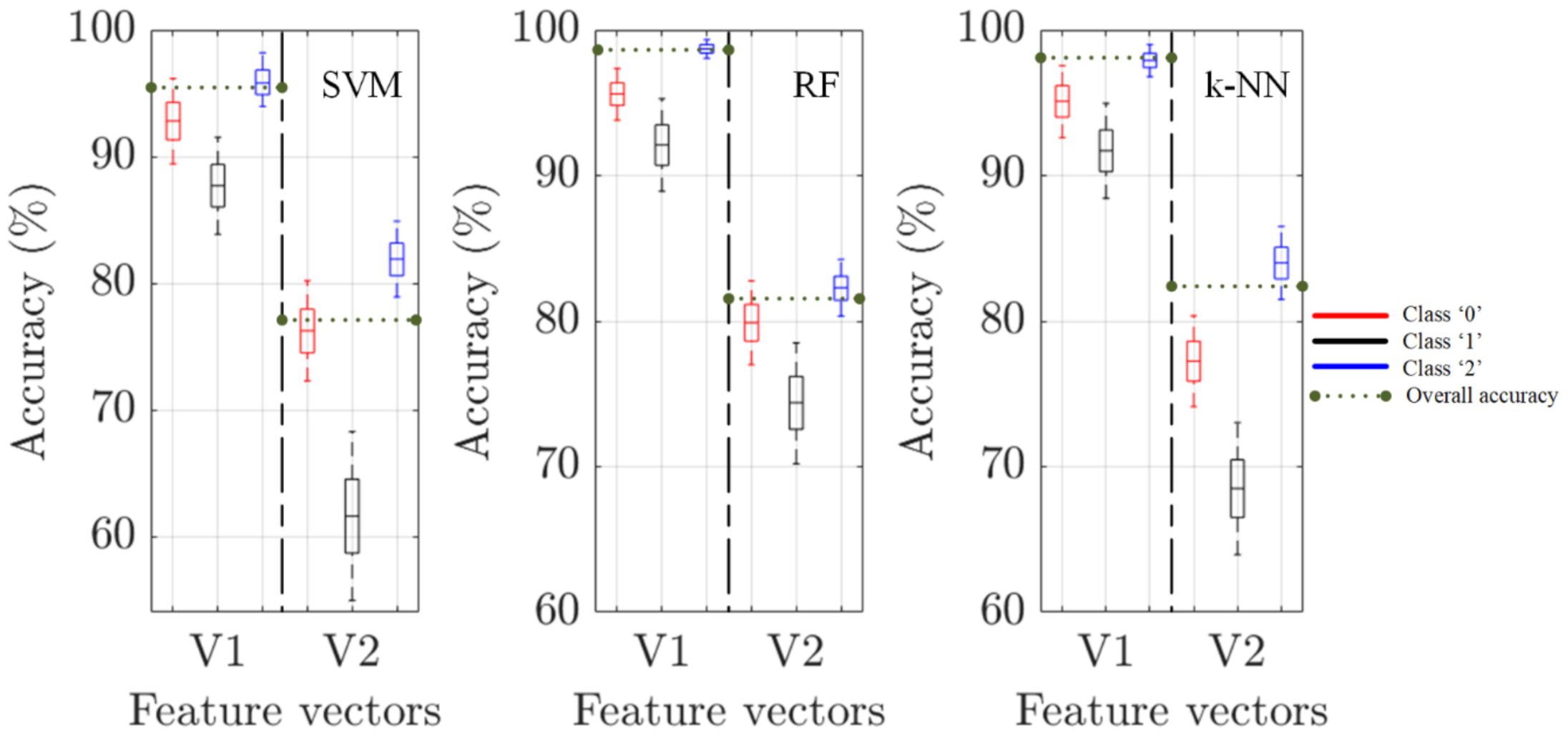
The weighted accuracy of detecting each fault class is presented in Figure 6, evaluating the performance for all the three individual classes independent of the number of observations considering a balanced dataset. Each class’s accuracy is calculated to ensure that each label is correctly predicted and that no specific class dominates the overall accuracy. V1 outperforms V2 in all cases, and the combination of V1 and RF seems to be the best across the entire validation set. It is noticeable that ‘Class 1’ detection accuracy is lower than in the other two classes. We assume that some micro-cracks and finger failures are falsely predicted as ‘No failures’. The reasons for this false prediction differ between the two vectors. As the intensity and contrast of Class 1 are similar to healthy cells, feature vector V1 is less sensitive to this fault. When V2 is used, it seems that as Class 1 failures affect only a relatively small percentage of the acquired image, they are sometimes classified as statistical noise.
Figure 6 also displays the computed accuracy for each of the computed ML classifiers. The overall accuracy values (see Table 3) give an unbiased estimate for correctly predicting the images’ actual class labels from the final tuned algorithm. It should be noted that the weighted average accuracy of all the classes (92.1% (SVM), 95.4% (RF), and 94.9% (k-NN)) is lower than the overall accuracy (96.7% (SVM), 99.2% (RF), 98.4% (k-NN)) for the V2 feature vector. It gives equal contributions to the three classes’ predictive performance, which are independent of their number of observations, unlike those used to compute the overall accuracy. The V1 feature vector’s overall accuracy indicates that the overall performance is high compared to that of the V2 feature vector, even though the classifiers underperform in the individual class 1 of all three classes. Furthermore, other output metric parameters (precision, recall, true positives, false positives and more) are calculated (see Figure A1) and the performance of the developed vectors are evaluated.
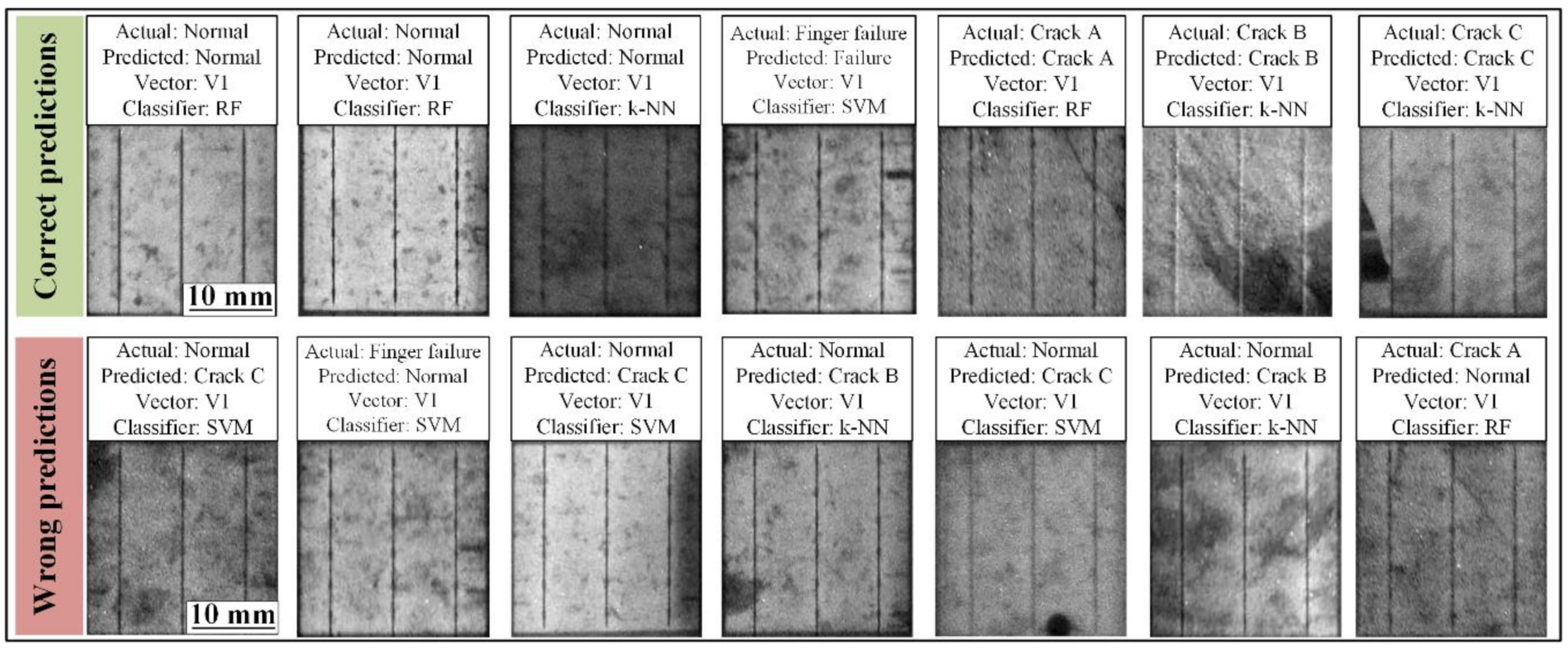
Figure 7 presents represented images with their actual and predicted labels. We analyze the falsely predicted images to evaluate the mislabels. Interestingly, many of the wrongly labeled cases are due to other failures (such as striation rings) that have not been classified in this study. The algorithms have classified these images as Class 0 or Class 1, although the actual classification (by the trainer) is Class 2 (no failure). This can be easily addressed by adding new classes. Other cases were misclassified due to a small difference between neighboring pixel values in the EL image identified as statistical noise. This can be improved using higher resolution images. It should be noted that standard deviation, inactive area, sensitivity peak, entropy, and kurtosis are the most sensitive parameters for Class 0 failure type. In contrast, skewness, standard deviation, and kstat parameters played a significant role in predicting Class 1 failures.

5. Conclusions

The early detection of defects as cracks, micro-cracks, and finger failures in solar cells is important for the production of PV modules. Analyzing EL images to locate and identify these failures is typically a time-consuming manual process and requires expert knowledge.
In this paper, a machine learning-based failure identification method was presented. The technique uses EL images to classify three classes of faults using a feature vector based on statistical parameters. The feature vector has a significant advantage over the standard feature vector that uses all the main output metrics. The developed feature vector achieves an accuracy and F1-score similar to state-of-the-art reported results despite a smaller dataset. As the proposed method requires less computation power and time, it will be valuable for outdoor EL inspection using intelligent unmanned aerial vehicles or drone-mounted systems.

Author Contributions

Conceptualization: H.R.P.; Investigation: H.R.P., Y.B., and Z.H.; Methodology: H.R.P. and F.V.; Project administration: D.S.; Resources: S.W.; Software: H.R.P., Y.B.; Supervision: Z.H., and S.S.; Validation: Z.H., Y.B.; Writing—original draft, H.R.P.; Writing—review & editing: Z.H., Y.B., S.S., F.V., G.A.D.R.B., P.B.P., T.K., and D.S. All authors have read and agreed to the published version of the manuscript.

Funding

This research was partially funded by Innovation Fund Denmark, grant number: ID 6154-00012B and Australian Renewable Energy Agency (ARENA), grant number: ID 2020/RND016.

Acknowledgments

The Innovation Fund Denmark partially supported this study within the research project DronEL-“Fast and accurate inspection of large PV plants using aerial drone imaging” (ID 6154-00012B). The Australian Renewable Energy Agency (ARENA) funded a part of the project (Grant ID 2020/RND016). The authors also would like to express their gratitude to the PI Berlin Group for providing the EL images.

Conflicts of Interest

The authors declare no conflict of interest. Moreover, the funders had no role in the study’s design; in the collection, analyses, or interpretation of data; in the writing of the manuscript, or in the decision to publish the results.

Appendix A

Table A1. Derived statistical parameters from the pixel intensity histogram of an EL cell image [49,50].
Statistical ParametersFormulae
Cell level EL pixels ρ E L c e l l k , i   = n i k n k , 0 i < L ,   1 k N c
Mean μ c e l l k   = 1 L · i = 0 L 1 ρ E L c e l l k , i
Standard deviation (SD) σ c e l l k   = 1 L · ( i = 0 L 1 ρ E L c e l l k , i μ c e l l k ) 2
Skewness γ c e l l k   = 1 L · i = 0 L 1 ( ρ E L c e l l k , i μ c e l l k σ c e l l k ) 3
Kurtosis κ c e l l k   = 1 L · i = 0 L 1 ( ρ E L c e l l k , i μ c e l l k σ c e l l k ) 4
Inactive area I E L c e l l k %   = 100 · i = 0 T H ρ E L c e l l k , i
Sensitivity peak P e a k k   = max ρ E L c e l l k , i
Full-width F W k   = x 100 · max ρ E L c e l l k , i x 100 · min ρ E L c e l l k , i
Entropy ϵ c e l l k   = i = 0 L 1 ρ E L c e l l k , i · log 10 ρ E L c e l l k , i
Angular second moment A S M c e l l k   = i = 0 L 1 ρ E L c e l l k , i
Kstat k n   i s   t h e   u n i q u e   s y m m e t r i c   u n b i a s e d   e s t i m a t o r   o f   t h e   n t h   k s t a t i s t i c
Variation c o m p u t e s   t h e   c o e f f i c i e n t   o f   v a r i a t i o n ,   t h e   r a t i o   o f   b i a s e d   S D   t o   m e a n
Median c o m p u t e s   t h e   50 %   p e r c e n t i l e   f r o m   t h e   h i s t o g r a m   o f   t h e   c e l l
Percentiles c o m p u t e s   t h e   10 %   a n d   90 %   p e r c e n t i l e   f r o m   t h e   h i s t o g r a m   o f   t h e   c e l l
Zscore c o m p u t e s   t h e   z s c o r e   o f   e a c h   s a m p l e   v a l u e ,   r e l a t i v e   t o   t h e   m e a n   a n d   S D
Error of measurement e v a l u a t e s   t h e   s t a n d a r d   e r r o r   o f   t h e   c o m p u t e d   m e a n
The solar cells in the test modules used in this study were analyzed individually by automatically extracting the cell-level EL images. From each solar cell image, the cell-level EL intensity distribution, p E L C e l l (k, i), is calculated [49], where k is the solar cell number, and i is the intensity level (gray level occurrences) at a particular pixel position in a solar cell image. L is the maximum intensity level (256), while Nc is the number of solar cells in a module. nik is the number of occurrences of gray level i in the cell k, while nk is the total number of pixels in the image of the cell k.
From the cell-level image, distribution parameters are calculated for each solar cell, such as STD, mean, median, skewness, kurtosis, as defined in Table A1.

Appendix B

Figure A1 provides an overall performance evaluation of V1 and V2 and highlights the correlation between the actual and predicted labels. The percentage of solar cells predicted incorrectly in the different class categories is significantly lower for V1. The recall value calculated by the algorithm is highlighted in gold and represents the row (Total Col). Even though V2 measures an 81.9% recall value, using V1 with the most dominant parameters improves the performance to a overall recall value of 97.9% for the RF classifier (see Table 3). A similar evaluation is inferred by correctly classifying the actual positive outcome, which correlates with the predicted positive outcome calculated from Figure A1 and reports as precision value highlighted in lavender and representing the column (Total line). As expected, the V1 feature vector achieved a precision value of 99.2% (RF classifier), outperforming the combined approach (V2) with 86.2%.
Figure A1. Confusion matrices of the implemented feature vectors (V1,V2) fed as an input to the RF ML classifier.
Applsci 10 08834 g0a1

References

  1. Haegel, N.M.; Atwater, H.; Barnes, T.; Breyer, C.; Burrell, A.; Chiang, Y.-M.; De Wolf, S.; Dimmler, B.; Feldman, D.; Glunz, S.; et al. Terawatt-scale photovoltaics: Transform global energy. Science 2019, 364, 836–838. [Google Scholar] [CrossRef] [PubMed] [Green Version]
  2. Green, M. Photovoltaic technology and visions for the future. Prog. Energy 2019, 1, 013001. [Google Scholar] [CrossRef]
  3. Köntges, M.; Kurtz, S.; Packard, C.; Jahn, U.; Berger, K.; Kato, K.; Kazuhilo, F.; Thomas, F.; Liu, H.; van Iseghem, M. IEA-PVPS Task 13: Review of Failures of Photovoltaic Modules; SUPSI: Manno, Switzerland, 2014. [Google Scholar]
  4. Spataru, S.; Hacke, P.; Sera, D. Automatic detection and evaluation of solar cell micro-cracks in electroluminescence images using matched filters. In Proceedings of the 2016 IEEE 43rd Photovoltaic Specialists Conference (PVSC); Institute of Electrical and Electronics Engineers (IEEE), Portland, OR, USA, 5–10 June 2016; pp. 1602–1607. [Google Scholar]
  5. Spataru, S.; Hacke, P.; Sera, D.; Glick, S.; Kerekes, T.; Teodorescu, R. Quantifying solar cell cracks in photovoltaic modules by electroluminescence imaging. In Proceedings of the 2015 IEEE 42nd Photovoltaic Specialist Conference (PVSC), Institute of Electrical and Electronics Engineers (IEEE), New Orleans, LA, USA, 14–19 June 2015; pp. 1–6. [Google Scholar]
  6. Dhimish, M.; Holmes, V.; Mehrdadi, B.; Dales, M. The impact of cracks on photovoltaic power performance. J. Sci. Adv. Mater. Devices 2017, 2, 199–209. [Google Scholar] [CrossRef]
  7. Kajari-Schršder, S.; Kunze, I.; Kšntges, M. Criticality of Cracks in PV Modules. Energy Procedia 2012, 27, 658–663. [Google Scholar] [CrossRef] [Green Version]
  8. Akram, M.W.; Li, G.; Jin, Y.; Chen, X.; Zhu, C.; Zhao, X.; Khaliq, A.; Faheem, M.; Ahmad, A. CNN based automatic detection of photovoltaic cell defects in electroluminescence images. Energy 2019, 189, 116319. [Google Scholar] [CrossRef]
  9. De Rose, R.; Malomo, A.; Magnone, P.; Crupi, F.; Cellere, G.; Martire, M.; Tonini, D.; Sangiorgi, E. A methodology to account for the finger interruptions in solar cell performance. Microelectron. Reliab. 2012, 52, 2500–2503. [Google Scholar] [CrossRef]
  10. Zafirovska, I.; Juhl, M.K.; Weber, J.W.; Wong, J.; Trupke, T. Detection of Finger Interruptions in Silicon Solar Cells Using Line Scan Photoluminescence Imaging. IEEE J. Photovolt. 2017, 7, 1496–1502. [Google Scholar] [CrossRef]
  11. Breitenstein, O.; Bauer, J.S.; Bothe, K.; Hinken, D.; Muller, J.; Kwapil, W.; Schubert, M.C.; Warta, W. Can luminescence imaging replace lock-in thermography on solar cells and wafers? IEEE J. Photovolt. 2011, 1, 159–167. [Google Scholar] [CrossRef]
  12. Fuyuki, T.; Kondo, H.; Yamazaki, T.; Takahashi, Y.; Uraoka, Y. Photographic surveying of minority carrier diffusion length in polycrystalline silicon solar cells by electroluminescence. Appl. Phys. Lett. 2005, 86, 262108. [Google Scholar] [CrossRef]
  13. Köntges, M.; Kunze, I.; Kajari-Schröder, S.; Breitenmoser, X.; Bjørneklett, B. The risk of power loss in crystalline silicon based photovoltaic modules due to micro-cracks. Sol. Energy Mater. Sol. Cells 2011, 95, 1131–1137. [Google Scholar] [CrossRef]
  14. Deitsch, S.; Christlein, V.; Berger, S.; Buerhop-Lutz, C.; Maier, A.; Gallwitz, F.; Riess, C. Automatic classification of defective photovoltaic module cells in electroluminescence images. Sol. Energy 2019, 185, 455–468. [Google Scholar] [CrossRef] [Green Version]
  15. Fada, J.S.; Hossain, M.A.; Braid, J.L.; Yang, S.; Peshek, T.J.; French, R.H. Electroluminescent Image Processing and Cell Degradation Type Classification via Computer Vision and Statistical Learning Methodologies. In Proceedings of the 2017 IEEE 44th Photovoltaic Specialist Conference (PVSC), Institute of Electrical and Electronics Engineers (IEEE), Washington, DC, USA, 25–30 June 2017; pp. 3456–3461. [Google Scholar]
  16. Bhoopathy, R.; Kunz, O.; Juhl, M.K.; Trupke, T.; Hameiri, Z. Outdoor photoluminescence imaging of photovoltaic modules with sunlight excitation. Prog. Photovolt. Res. Appl. 2018, 26, 69–73. [Google Scholar] [CrossRef]
  17. Alpaydin, E. Introduction to Machine Learning; The MIT Press: Cambridge, MA, USA, 2010. [Google Scholar]
  18. Bishop, C.M. Pattern Recognition and Machine Learning (Information Science and Statistics); Springer: London, UK, 2006. [Google Scholar]
  19. Karimi, A.M.; Fada, J.S.; Liu, J.; Braid, J.L.; Koyuturk, M.; French, R.H. Feature Extraction, Supervised and Unsupervised Machine Learning Classification of PV Cell Electroluminescence Images. In Proceedings of the 2018 IEEE 7th World Conference on Photovoltaic Energy Conversion (WCPEC) (A Joint Conference of 45th IEEE PVSC, 28th PVSEC & 34th EU PVSEC), Institute of Electrical and Electronics Engineers (IEEE), Waikoloa Village, HI, USA, 10–15 June 2018; pp. 0418–0424. [Google Scholar]
  20. Sun, M.-J.; Lv, S.; Zhao, X.; Li, R.; Zhang, W.; Zhang, X. Defect Detection of Photovoltaic Modules Based on Convolutional Neural Network. In Proceedings of the Lecture Notes of the Institute for Computer Sciences, Social Informatics and Telecommunications Engineering; Springer Science and Business Media LLC: Cham, Switzerland, 2018; pp. 122–132. [Google Scholar]
  21. Tseng, D.-C.; Iu, Y.-S.; Chou, C.-M. Automatic Finger Interruption Detection in Electroluminescence Images of Multicrystalline Solar Cells. Math. Probl. Eng. 2015, 2015, 1–12. [Google Scholar] [CrossRef]
  22. Mantel, C.; Villebro, F.; Benatto, G.A.D.R.; Parikh, H.R.; Wendlandt, S.; Hossain, K.; Poulsen, P.B.; Spataru, S.; Sera, D.; Forchhammer, S. Machine learning prediction of defect types for electroluminescence images of photovoltaic panels. In Applications of Machine Learning; International Society for Optics and Photonics: Bellingham, WA, USA, 2019; pp. 1–9. [Google Scholar]
  23. Hsu, C.-C.; Lin, C.-W. CNN-Based Joint Clustering and Representation Learning with Feature Drift Compensation for Large-Scale Image Data. IEEE Trans. Multimed. 2017, 20, 421–429. [Google Scholar] [CrossRef] [Green Version]
  24. Tsai, D.-M.; Wu, S.-C.; Chiu, W.-Y. Defect Detection in Solar Modules Using ICA Basis Images. IEEE Trans. Ind. Inform. 2013, 9, 122–131. [Google Scholar] [CrossRef]
  25. Anwar, S.A.; Abdullah, M.Z. Micro-crack detection of multi-crystalline solar cells featuring an improved anisotropic diffusion filter and image segmentation technique. EURASIP J. Image Video Process. 2014, 2014, 15. [Google Scholar] [CrossRef] [Green Version]
  26. Li, X.; Wang, J.; Chen, Z. Intelligent fault pattern recognition of aerial photovoltaic module images based on deep learning technique. J. Syst. Cybern. Inf. 2018, 16, 67–71. [Google Scholar]
  27. Li, X.; Yang, Q.; Lou, Z.; Yan, W. Deep Learning Based Module Defect Analysis for Large-Scale Photovoltaic Farms. IEEE Trans. Energy Convers. 2019, 34, 520–529. [Google Scholar] [CrossRef]
  28. Ding, S.; Yang, Q.; Li, X.; Yan, W.; Ruan, W. Transfer learning based PV module defect diagnosis using aerial images. In Proceedings of the 2018 International Conference on Power System Technology (POWERCON), Guangzhou, China, 6–8 November 2018; pp. 4245–4250. [Google Scholar]
  29. Chen, H.; Pang, Y.; Hu, Q.; Liu, K. Solar cell surface defect inspection based on multi-spectral convolutional neural network. J. Intell. Manuf. 2020, 31, 453–468. [Google Scholar] [CrossRef] [Green Version]
  30. Luo, Z.; Cheng, S.Y.; Zheng, Q. GAN-Based Augmentation for Improving CNN Performance of Classification of Defective Photovoltaic Module Cells in Electroluminescence Images. IOP Conf. Ser. Earth Environ. Sci. 2019, 354, 012106. [Google Scholar] [CrossRef] [Green Version]
  31. Rousseeuw, P. Least median of squares regression. J. Am. Stat. Assoc. 1984, 79, 871–880. [Google Scholar] [CrossRef]
  32. Malis, E.; Vargas, M. Deeper Understanding of the Homography Decomposition for Vision-Based Control; INRIA: Paris, France, 2007. [Google Scholar]
  33. Szeliski, R. Computer Vision: Algorithms and Applications; Springer-Verlag: London, UK, 2010. [Google Scholar]
  34. Perspective Control Correction with Mathworks. Available online: https://se.mathworks.com/matlabcentral/fileexchange/35531-perspective-control-correction/ (accessed on 5 April 2020).
  35. Mantel, C.; Villebro, F.; Parikh, H.; Spataru, S.; Benatto, G.A.D.R.; Sera, D.; Poulsen, P.B.; Forchhammer, S. Method for Estimation and Correction of Perspective Distortion of Electroluminescence Images of Photovoltaic Panels. IEEE J. Photovolt. 2020, 10, 1797–1802. [Google Scholar] [CrossRef]
  36. Ali, U.; Mahmood, M.T. Analysis of Blur Measure Operators for Single Image Blur Segmentation. Appl. Sci. 2018, 8, 807. [Google Scholar] [CrossRef] [Green Version]
  37. Deitsch, S.; Buerhop-Lutz, C.; Maier, A.; Gallwitz, F.; Riess, C. Segmentation of photovoltaic module cells in electroluminescence images. Clin. Orthop. Relat. Res. 2018, 1806, 455–468. [Google Scholar]
  38. Hearst, M.A.; Dumais, S.T.; Osuna, E.; Platt, J.; Scholkopf, B. Support vector machines. IEEE Intell. Syst. Their Appl. 2019, 13, 18–28. [Google Scholar] [CrossRef] [Green Version]
  39. Applying Supervised Learning with Mathworks. Available online: https://se.mathworks.com/campaigns/offers/machine-learning-with-matlab.html (accessed on 21 August 2020).
  40. Linge, S.; Langtangen, H.P. Programming for Computations—Python: A Gentle Introduction to Numerical Simulations with Python; Springer: London, UK, 2016. [Google Scholar]
  41. Mckinney, W. Pandas: A foundational python library for data analysis and statistics. Python High Perform. Sci. Comput. 2011, 4, 1–9. [Google Scholar]
  42. Ziegler, A.; James, R.G.; Witten, D.; Hastie, T.; Tibshirani, R. An introduction to statistical learning with applications. Biometr. J. 2016, 58, 440. [Google Scholar]
  43. Kotsiantis, S. Supervised machine learning: A review of classification techniques. Informatica 2007, 31, 249–268. [Google Scholar]
  44. Breiman, L. Random forests. Mach. Learn. 2001, 45, 5–32. [Google Scholar] [CrossRef] [Green Version]
  45. Breiman, L.; Freidman, J.; Stone, C.J.; Olshen, R.A. Classification and Regression Trees; CRC Press: Boca Raton, FL, USA, 1984. [Google Scholar]
  46. VanderPlas, J. Python Data Science Handbook; O’Reilly Media Inc.: Sebastopol, CA, USA, 2016. [Google Scholar]
  47. Powers, D. Evaluation: From precision, recall and f-factor to ROC, informedness, markedness, and correlation. Mach. Learn. Technol. 2008, 2, 37–63. [Google Scholar]
  48. Buratti, Y.; Dick, J.; Le Gia, Q.; Hameiri, Z. A Machine Learning Approach to Defect Parameters Extraction: Using Random Forests to Inverse the Shockley-Read-Hall Equation. In Proceedings of the 2019 IEEE 46th Photovoltaic Specialists Conference (PVSC), Institute of Electrical and Electronics Engineers (IEEE), Chicago, IL, USA, 16–21 June 2019; pp. 3070–3073. [Google Scholar]
  49. Spataru, S.; Parikh, H.; Hacke, P.; Benatto, G.A.d.R.; Sera, D. Quantification of solar cell failure signatures based on statistical analysis of electroluminescence images. In Proceedings of the 33rd European Photovoltaic Solar Energy Conference and Exhibition: EU PVSEC, Amsterdam, The Netherlands, 25–29 September 2017; pp. 1466–1472. [Google Scholar]
  50. Statistical Functions Using Scipy.Stats. Available online: https://docs.scipy.org/doc/scipy/reference/stats.html (accessed on 9 September 2020).
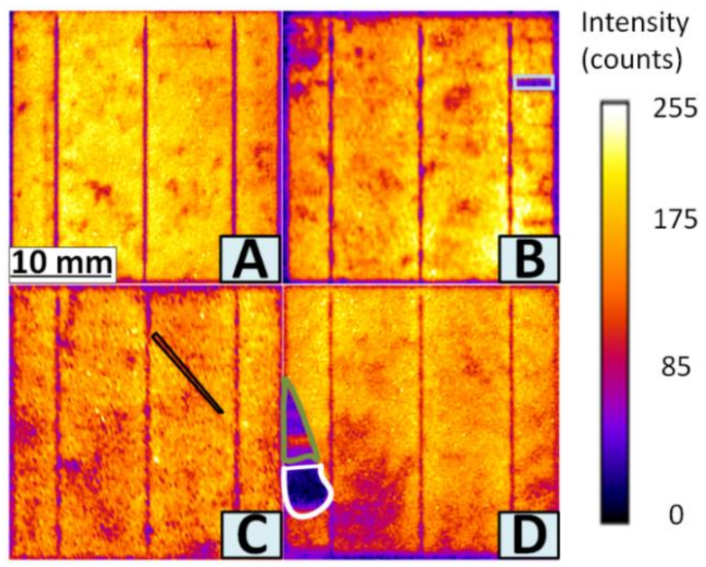
Figure 1. EL cell images inflicted with different faults: (A) no failures; (B) finger failures (region marked with light blue); (C) micro-crack Mode A (black); (D) cracks Mode B (olive green) and Mode C (white).
Applsci 10 08834 g001
Figure 2. The image processing procedure used in this study: (A) acquired raw EL measurements; (B) the prospectively corrected normalized image; (C) busbar identification; (D) solar cell extraction; and (E) busbar removal.
Applsci 10 08834 g002
Figure 3. The training procedure used in this study.
Applsci 10 08834 g003
Figure 4. (A) Extracted statistical parameters (V1; 16 features); (B) combined pixel intensity histogram and statistical parameters (V2; 271 features) used as inputs for three ML classifiers.
Applsci 10 08834 g004
Figure 5. Statistical boxplot of the F1 score for the three ML classifiers.
Applsci 10 08834 g005
Figure 6. The accuracy scores of the developed feature vectors for the three ML classifiers.
Applsci 10 08834 g006
Figure 7. Qualitative evaluation of the correct and wrong predictions based on the proposed algorithms actual and predicted class labels.
Applsci 10 08834 g007
Table 1. Defect classification.
Module ImagesCell Images‘Class 0’‘Class 1’‘Class 2’
75345,90675662944,521
Balanced data-set2185756629800
Table 2. Extracted output metrics and their definition.
ParameterAccuracy (%) Recall   ( r ) (%) Precision   ( p ) (%)F1 Score (%)
Formulae t p   +   t n t p   +   f p   +   f n   +   t n t p t p   +   f n t p t p   +   f p ( 2 · p · r p   +   r )
t p : T r u e   p o s i t i v e , f p : F a l s e   p o s i t i v e , f n : F a l s e   n e g a t i v e , t n : T r u e   n e g a t i v e .
Table 3. Overall results of implemented feature vectors and the different ML classifiers.
Feature VectorsStatistical Parameters (V1)Pixel Intensity Histogram + Statistical Parameters (V2)
ML ClassifiersSVMRFk-NNSVMRFk-NN
F1 score (%)94.398.397.180.983.982.1
Accuracy (%)96.799.298.476.683.183.9
Recall (%)93.897.996.379.981.980.6
Precision (%)92.899.297.982.986.285.5
Table 4. Summary of the performance of various automated fault classification for EL images.
Research ArticleMethod (Vector)ClassifierF1score (%)Accuracy (%)Detected DefectsEL Cell Images (Dataset)
This studyStatistical parameters (V1)RF98.399.6Cracks B and C
k-NN97.198.5micro-crack A2185
SVM94.396.7finger failures
Cracked, busbar
[19]Haralicks featuresSVM9898.9corroded, edge and busbar darkened,6264
CNN9798.2
Spectral clustering
[21]ROI locationk-mean method92.199.1Interrupted finger defects ----
Stochastic gradient descentSVM---98.7
[15]MLP-ANN---98.1Cracked, corroded14,200
RF---96.9
NAG based learning Cracks (normal, linear, cross, flaky, broken)
[20]CNN---98.46120
Isolated deep learning
[8]CNN91.993Different defects>7872
Transfer learning via t-SNE Material defects, grid fingers, deep and microcracks, cell degradation
[14]CNN88.488.42624
Material defects, grid fingers, deep and microcracks, cell degradation
[14]Kaze/VGGSVM82.582.42624
Hough region detection Cracks B and C
[22]SVM5.199.7micro-crack A47,244
RF4.496.7finger failures
Percentile region detection Cracks B and C
[22]RF6.696.5micro-crack A47,244
SVM4.199.7finger failures
Publisher’s Note: MDPI stays neutral with regard to jurisdictional claims in published maps and institutional affiliations.