A Mathematical Model for the Scheduling of Virtual Microgrids Topology into an Active Distribution Network


1
IREC Catalonia Institute for Energy Research, C. Jardins de les Dones de Negre, 1, Pl. 2a, 08930 Sant Adrià del Besòs, Spain
2
Convertidors Estàtics i Accionaments (CITCEA-UPC), Department of Electrical Engineering, Universitat Politècnica de Catalunya ETS d′Enginyeria Industrial de Barcelona, C. Avinguda Diagonal, 647, Pl. 2, 08028 Barcelona, Spain
3
Industrial Engineering Department, University of Santiago de Chile, Avenida Ecuador 3769, Santiago 9170124, Chile
4
Department of Statistics and Operations Research, Universitat Politècnica de Catalunya (UPC), Carrer Jordi Girona 1, 08034 Barcelona, Spain
*
Authors to whom correspondence should be addressed.
Appl. Sci. 2020, 10(20), 7199; https://doi.org/10.3390/app10207199
Submission received: 22 September 2020
/
Revised: 5 October 2020
/
Accepted: 9 October 2020
/
Published: 15 October 2020
(This article belongs to the Special Issue Resilient and Sustainable Distributed Energy Systems)
Abstract
:This article presents a method based on a mathematical optimization model for the scheduling operation of a distribution network (DN). The contribution of the proposed method is that it permits the configuration and operation of a DN as a set of virtual microgrids with a high penetration level of distributed generation (DG) and battery energy storage systems (BESS). The topology of such virtual microgrids are modulated in time in response to grid failures, thus minimizing load curtailment, and maximizing local renewable resource and storage utilization as well. The formulation provides the load reduced by bus to balance the system at every hour and the global probability to present energy not supplied (ENS). Furthermore, for every bus, a flexibility load response range is considered to avoid its total load curtailment for small load reductions. The model has been constructed considering a linear version of the AC optimal power flow (OPF) constraints extended for multiple periods, and it has been tested in a modified version of the IEEE 33-bus radial distribution system considering four different scenarios of 72 h, where the global energy curtailment has been 27.9% without demand-side response (DSR) and 10.4% considering a 30% of flexibility load response. Every scenario execution takes less than a minute, making it appropriate for distribution system operational planning.
1. Introduction
The concept of resilience has been increasingly used in the literature related to distribution networks (DN) with high penetration levels of distributed energy resources (DER), with an interest in providing greater autonomy and flexibility in the face of unexpected power generation situations [1]. In this context, microgrids (MG) play a relevant role in the transition process to smart grids because they offer an electrical structure that allows for improving the monitoring and management control of the renewable resources on a small scale [2,3]. However, following the definition of MGs given by the U.S. Department of Energy [4], a fixed electrical boundary may not be exploiting all the flexibility that an MG provides.
The concept of virtual microgrids (VM) with dynamic boundaries has begun to emerge as an alternative for increasing the resilience of conventional DNs [5,6] based on the IEEE Standard 1547.4 [7], which establishes that the reliability and operation of DNs can be improved by dividing the DN into multiple “isolated systems”. Discussions regarding a common definition of VMs with dynamic limits continue. However, there are some characteristics in common in the work that has been done; the work by [8] proposes that a VM is developed from a centralized DN, and possesses the same features of an MG but with a flexible structure based on virtual boundaries. The work done by [9] considers a dynamic MG as one with flexible boundaries that expand or shrink to maintain the balance between power generation and power consumption. The work in [10] considers the paradigm of a dynamic MG as a mechanism to continuously partition a DN based on the balance between electricity generation and demand.
The key factor in the definitions above is the capability of the DN to find the best partition such that it minimizes the load curtailment, and balances the power system under failure or unbalanced scenarios produced by the stochastic behavior of the DG. Likewise, this responsiveness is based on the autonomy level of the active distribution network (ADN), i.e., the installed capacity of DG and batteries. Thus, the higher the installed capacity is, the higher the autonomy would be. However, to meet 100% of the electricity load with only DERs requires a high investment, which could make the implementation of these technologies in a DN unprofitable [11] and/or bring voltage and frequency issues [12]. Therefore, in most cases, a trade-off occurs between the energy provided by DERs and the utility grid, where the grid helps the DERs fill the energy gap in the critical hours and decreases the installed capacity needed of the renewable resources [13]. Thus, the necessity of partitioning the ADN into VMs under failures of the utility grid increases because, under failure scenarios, the gap cover by the grid, when the DERs do not meet the load, will produce an unbalanced system. That is, unless the ADN faces this issue by dividing itself into virtual “island systems”.
Some clustering techniques [14,15] and methodologies have been applied to find an optimal partition that allows the network to adopt this dynamic structure. A Genetic Algorithm has been used in [16] to partition a DN to minimize the energy exchange between MGs. The work done by [8] proposes a hierarchical bottom-to-top algorithm based on community detection [17] using an Electrical Coupling Strength as modularity index, which is defined as a composite weighted factor for the analysis of the electrical connection, to size the partition quality. In [18], a Greedy and Particle Swarm Optimization (PSO) algorithm based on community detection is used to find sub-communities through an index based on the voltage sensitivity matrix and the active/reactive power. The Greedy algorithm is used to find the best partition and the PSO to manage the voltage control for each MG. The electrical distance is used in [19,20] to partition a DN into sub-systems. A control system based on Kruskal’s algorithm from graph theory is presented in [21] to synchronize and separate DN into multiple island systems to keep the system balanced. In [22], a bi-level optimization problem is presented to transform an active DN in multiple MGs using spectral graph theory to define the maximum numbers of sub-networks through a mixed-integer nonlinear problem (MINLP), and a second lower-level problem is presented to measure the reliability of the MGs formed by the upper-level. An optimal scheduling model is presented in [23] to address dynamic MG reconfiguration, where a linear version of the AC-OPF is proposed and uses the bender decomposition method to decompose and coordinate the grid-connected system and isolated operation through a master problem and sub-problem, respectively.
The existing literature sets out that the techniques used until now for partition and dynamic MG reconfiguration are based on mostly spectral graph theory and hierarchical and community detection algorithms. Nevertheless, to the best of our knowledge, there is not a single mathematical optimization model which provides the DN dynamic reconfiguration scheduling, based on demand side response (DSR) and load curtailment, such that it prevents widespread blackouts as a result of low power generation or network failures, for DN with high penetration of DG and BESS.
In order to extend the literature, the proposed model addresses this issue and provides additional information for the distribution system operations (DSO). The main contributions of this article are summarized as follows:
- A new mathematical optimization model is presented which provides the virtual microgrid topology scheduling of an ADN considering the load curtailment and its flexibility response as the main criteria to partition an unbalanced system into several VMs balanced, with a computational time short enough to ease its adoption by DSO in their usual operational procedures.
- We have extended the literature related to the partitioning methods in order to obtain VMs with dynamic boundaries, leaving the algorithms based on hierarchical or graph theory, and providing an optimization linear model.
- A quantification of the weaker nodes in terms of the probability of the node to not meet the load under consecutive scenarios, and the size of the energy not supplied which is a useful value in flexibility markets.
The rest of the paper is organized as follows. Section 2 describes the problematic where the mathematical model is situated, and the methodology follows to validate the model under different scenarios. Section 3 presents the mathematical model with the nonlinear constraints already linearized. In Section 4, the model proposed is tested in a case of study and the results are mentioned and discussed. In addition, finally, the conclusions are presented in Section 5.
2. Preliminaries
This section explains the problem the mathematical model addresses, together with the methodology the authors follow to create a proper test context. Furthermore, a comparison with the current literature is presented.
2.1. Problem Definition
Currently, the distribution and transmission systems are supported by different control mechanisms to face the deviation between electricity production and the load [24,25]. This work, typically managed by the transmission system operator (TSO), keeps the energy balancing through three types of control reserves which differ by the temporal space in which they are applied. The question thus arises: why partition a DN to face unexpected events if there are control mechanisms to prevent these kinds of issues? The answer is that the aim of using the resilience concept associated with the DN with high penetration levels of DERs is to dispense with these control mechanisms and be able to achieve self-adaptation to a failure of high impact on the grid [26]. Therefore, the ADN must be able to measure the energy amount that cannot be met due to the absence of the utility grid and to identify the load points which could be applied to a load curtailment in order to minimize the energy losses.
The DSR concept is related to the amount of energy which the ADN could reduce to avoid an unbalanced system under the absence of the utility grid [27]. i.e., if the ADN possesses the flexibility to reduce a percentage of its energy load, the global curtailment will be lower than the case of an ADN where there is no chance to reduce the load more than to zero to avoid an unbalanced system. However, the flexibility degree of the DSR must be known in advance by the ADN such that the model can decide when and how much load to reduce.
2.2. Related Works
The literature related to the optimal partition of an ADN, introduced above, is grouped into algorithm or optimization models to explain the main differences between the current methodologies and the formulation proposed.
The work presented by [14] makes an overview of the clustering techniques available in the literature, together with a brief summary of its applicability. Some of these algorithms have been used to partition a DN into MGs or VMs, for which the most relevant are those who use community detection [8,17,18,19,20] based on a different index, such as: electrical distance [19,20], electrical coupling strength [17], or voltage sensitivity matrix [18] because they allow an identification, through an index, of the weakest point of a DN and the use of these weakest points as limit points between clusters. These methodologies are powerful tools when the partition required is for fixed boundaries and the technical network constraints are considered. However, the limitation appears when the topology is variable through time and some new elements, such as BESS and DSR, are introduced into the ADN since these flexibility elements possess a variable impact that must be considered in a time horizon where the next step depends on the behavior of the previous step.
The optimization models are an alternative of the algorithms because they permit finding an optimal value and include elements external to the DN, such as the BESS and DSR. Nevertheless, their main drawbacks lay in the nonlinearity and non-convexity of the AC-OPF formulation, which significantly increases their computation burden [28,29] and prevent their direct application for multi-period problems in an operational context. Specifically, the MINLP includes, in its AC version, the cosine and sine functions, which are the main problem because the current solvers available in the market possess high execution times. Under this context, some linearization methods are applied to reduce the complexity of the AC-OPF [30,31,32,33], of which some have been used in clustering optimization problems. However, there are few publications that use optimization models for the scheduling of VMs. The work in [23] uses a linearization and bender decomposition method to tackle the formation of dynamic MGs for an ADN with a high penetration of DERs. However, it does this without considering a flexible response of the loads. On the other hand, [22] uses spectral graph theory in a bi-level optimization problem to find MG reconfiguration into a DN with 123-buses, but the formulation does not include storage systems and DSR, and it is not applied in a multi-period context. Therefore, considering the sparse literature on the topic, one of the goals of the model proposed here is to extend the literature related to the optimization models applied in a clustering method to form VMs, considering DSR to increase the resilience of an ADN, and regardless of the current external mechanism.
2.3. Methodology
The methodology followed in this article consists of two stages: the first one assumes the capacity and location that should have the DG and BESS into the DN. The second stage addresses the capability of the DN to face unexpected failures through the self-partition into VMs, which is the main contribution of this article.
The placement and sizing have been addressed separately in [13], where a novel algorithm presented allows finding an optimal solution to the capacity and location for different types of DGs and BESSs, considering a time horizon longer than 24 h and basing the formulation on an AC-OPF to include the technical constraints of the network (this is represented in the upper level of Figure 1). The lower level of the figure corresponds to the optimal topology of the DN in case the power energy is insufficient to meet the electricity load. Therefore, following Figure 1, the optimal model for the VMs topology scheduling (VMTS) is executed for scenarios of 72 h, where every hour has two possible results regarding the system: the first one being, where the capacity installed, weather conditions, and the electricity load are balanced, meaning that the DN does not need to be partitioned into VMs. However, for the second result, if the electricity load is not satisfied by the power generation of the DGs, the model finds the amount of energy load that must be reduced at each bus to balance the system, where every load point possesses a range of load that can be reduced. If the load curtailment exceeds this range, the load in that point is reduced to zero and the bus is isolated, coming in a bound of VM. Thus, for each hour where these conditions appear, the model provides the scheduling of the topology that must follow the DN to continuously balance the system, sacrificing, of course, a load curtailment that is minimizing on the objective function but avoiding an outage.
In order to make sure that the topologies found by the mathematical model are feasible for the classic AC-OPF problem, the loads associated with the isolated nodes are replaced by zeros and the buses are modified with a reduced load within its range of flexibility. The DN with the new set of loads is executed in a multi-period AC-OPF. Thus, the feasible solutions of the VMTS model are also feasible for the classic AC-OPF problem.
3. Optimal Model for Scheduling Virtual Microgrids Topology
The formulation explained in this article is a modified version of the model presented in our previous work [13], which uses as the main structure an AC-OPF extended to a multi-period and a linearization done by [28]. However, unlike [13], which finds the optimal place and location of DERs into a DN, the model here is focused on finding the scheduling of a dynamic topology of an ADN to face lower generation scenarios or failure on the utility grid, through the minimization of the load curtailment in order to find the weakest nodes, and identify eventual flexibilities. The model is explained in two subsections; the first one corresponds to the base structure to find the proper topology of the ADN to face unbalance issues without taking into account a flexible demand response, and a second section, where the power consumption is not a parameter anymore but a variable, in order to include flexibility on demand.
3.1. Model without Demand Flexibility
The virtual microgrids topology scheduling (VMTS) model is described as follows:
The objective function in Equation (1) minimizes the active () and reactive () power not supplied, and the active () and reactive () power flow between the nodes. Thus, this structure allows us to:
- Promote the fulfillment of the electricity load since the positive variables and are penalized () when their values are greater than zero, if and only if, the power generation and the energy storage is not enough to meet the load.
- Prioritize the loads with or closer to a DG or BESS when it is not a chance to meet the power consumption through the minimization of the flow variables () and ().
In order to penalize the flow between nodes, the absolute value for the active and reactive power flow between nodes is considered, which can take negative and positive values depending on the flow direction, and because an absolute value requires a simple change of variable to become linear. On the other hand, the ENS penalization () is a parameter that is defined by the DSO regarding its power quality, i.e., if the ENS is more relevant than the energy losses through the lines, then is greater than the power flow through the lines. In the opposite case, must be equal to or lower than the power flow in lines.
The formulation constraints are as follows: Equations (2) and (3) correspond to active and reactive nodal power flow equations; therefore,
Both equations, and the remaining constraints, have already been linearized using the methodology presented in [28], holding the left side of these equations as the classic AC-OPF. However, on the right side, we consider the active power injected by the distributed resource (); a virtual active power (), which represents the power remaining to meet the load in case of low generation; the active power demanded by the node (), wherein this formulation is a parameter; and the power absorbed () or injected () from the battery to the grid. The same structure follows Equation (3).
The set of constraints from (4) to (7) correspond to the linear version of the active and reactive power flow equation which have been widely explained in previous AC-OPF formulations [13]; therefore, ,
Equation (8) represents the total power load which depends on the power supplied () and not supplied () in every node i, thus, the total load is composed by these two types of variable, where the power not supplied is penalized in the objective function, to ensure that is as small as possible. Equation (9), the power not-delivered (), bound the virtual power which represents the remaining power that it is needed to meet the total power load (see Equation (2)). Therefore, if the power generation is insufficient to provide the power required, the virtual power () variable fulfills this gap, being penalized in the objective function, if and only if this gap is equal to or lower than the power not supplied () in the node i. Constraints (10) and (11) describe the same logic except for the reactive power load.
Active and reactive power limits together with the voltage security constraints are considered in Equations (12)–(14); therefore, ,
Equation (12) makes sure that the voltage in each node and at every period is within the limits allowed. The parameters are squared due to the change of variable needed to linearize the original power flow equation. Constraints (13) establish the limits for the power injected by the DG in the node through two different parameters; corresponds to the total power capacity installed and is the power generated by the DG in a certain period, which is a normalized power generation curve. Therefore, Equation (13) establishes the maximum power that can be injected in Equation (2) at every hour, where follows the power generation behavior of a photovoltaic panel (PV)/wind turbine (WT), and it allows for including the stochastic behavior of the DG into the OPF constraints.
The sets of constraints (15)–(18) represent a linear version of the apparent power limit; therefore, ,
where:
Equations (15) and (16) emerge as a set of constraints which represent a polygon formed by lines that define a feasible region approximation of the original apparent power limit, which is a circle. Thus, the bigger the set , the closer the polygon will be to the circle.
To model the behavior of the batteries, the following constraints are added. Therefore, ,
The state of charge (SOC) for battery type l is defined in Equation (19) and is composed of the SOC of the previous period plus the energy injected and absorbed from the system with their respective efficiency factors. In order to maintain the structure of the formulation of our previous work [13], the SOC is in MWh and not in percentage, as usual; thus, the SOC represented in Equation (19) is bounded by / which are in % and are multiplied by the total capacity installed. In this way, the belongs only to the capacity range operation of the battery. Therefore, for a capacity of 10 MWh and a 90%/10% as operational limits, the will not be less than 1 MWh or greater than 9 MWh. On the other hand, the maximum power injected or taken from the DN for a certain period is explained in constraints (21) and (22) through which is multiplied by a binary variable representing when the battery is charging or discharging. In the case that the battery is discharging, i.e., , the maximum energy discharged must be equal to or lower than because the parameter is one when there is a battery in the node. Otherwise, if (a binary parameter) is zero, the constraints (23) are zero and all the Equations (19)–(22).
3.2. Model with Demand Flexibility
In this section, Equations (1), (2), (8) are rewritten in order to include the DSR into the model explained previously, and a new constraint is added to bound the flexibility degree of the energy demand:
Equation (24) is the new objective function for which, unlike (1), the amount of power consumption reduced () is minimized together with the energy flow and the active/reactive power not supplied, in order to balance the system. However, this new variable must be lower than or equal to the demand response of every load. Therefore,
where in Equation (25) represents the percentage of demand response of every load at every time, i.e., this vector parameter represents the flexibility of every load to reduce its demand. On this way, different flexibilities can be considered. For example, means that the bus 1 at 5th hour cannot reduce its demand. On the other hand, means that bus 2 at the 5th hour can reduce its demand by 15%. In addition, must be integrated into Equations (2) and (8) to keep the balance in the power flow equations, where the parameter passes to be an initial power consumption where the flexibility response is subtracted. Thus,
4. Results and Discussion
In this section, the two versions of the mathematical model are applied under four different scenarios of 72 h. Moreover, the impact of the DSR on the VMs formed by the model proposed is presented and discussed.
4.1. Case Study
A multi-period version of the PG&E 33-bus radial distribution network [34] has been used to test the model proposed. The sizing and location of the DERs have been separately obtained using the algorithm presented in our previous work [13], considering a connected-grid system because an autonomous network, i.e., the energy, is provided 100% by DERs; it is not a proper case of study to observe the capability of the ADN to form sub-systems when the grid fails. Therefore, using [13], the location and sizing have been set as shown in Figure 2.
In order to test the mathematical optimization model, four different 72-hour scenarios corresponding to each season of the year are taken into account to study the different topologies formed by the ADN when the system is disconnected from the utility grid and the weather conditions are not capable of supplying 100% of the power consumption. The weather resources are taken from historical data (a year and a time-step of 1[h]) of the Lugo, Galicia region in the north of Spain 2018; Ref. [35] for the wind speed, and [36] for the temperature and irradiance. The power generation data have been obtained using the modeling presented in [37] for the wind turbines, and the formulation used in [38] for PV panels. Thus, the energy demand and the power generation for the periods of study are presented in Figure 3. Every scenario of 72 hours has been chosen from the 8760 h available in the data set, with the aim to represent periods of 72 h with a high difference between both the power consumption and generation. Moreover, every curve has been normalized to respect the order of magnitude and comment on the power capability available. For example, the fourth period/scenario possesses a high-level wind resource, which means that the wind turbine will be able to produce energy at its maximum capacity. On the other hand, there are many consecutive hours that show a very low power capability for PV panels and wind turbines, which will force load curtailment and the partitioning of the ADN into sub-systems. The DSR parameter is set at 30% for every load at every time, i.e., every bus at every hour has the chance to reduce its load by 30%.
The mathematical model has been programmed in Python using Cplex as the main solver, and it has been run on an Intel Core i7-10510U CPU @ 1.80GHz 2.30 GHz with 16 GB memory and operative system Windows, 64 bit.
It should be noted that the goal of the case study is; (1) to size the DSR effect on the DN topology scheduling, and (2) to show the type of data provided by the model and how this information can be useful in terms of operational planning for DSO. It is important to mention this factor because the results depend exclusively on the DERs capacity, electricity demand, season, geographic location, weather conditions, and the DSR considered.
4.2. Model Performance
The mathematical formulation, explained in Section 3, has been compared with its MINLP version to observe the huge time differences between nonlinear and linear versions. Thus, Table 1 shows the times of execution for both models and their respective objective functions (OF). When the model is not multi-period, both formulations reach the same OF. However, when the model is extended to multi-periods, the computation burden for the MINLP increases faster than the MILP to the point that at hour 12 the time for the MINLP is around 5.5 h, which is much longer than the alternative version that takes only 3.79 s, keeping an error close to the 7%. Due to the exponential time execution increase for the MINLP version, Table 1 has been completed until hour 12 and not beyond. Nevertheless, the MILP running time for 72 h is close to a minute that puts it within the operational range of DSO.
4.3. Results
In order to improve the understanding of the data obtained from the model, the results are grouped as follows:
- Model operation explains how the model meets the energy load through the available resources and shows the role of the storage devices.
- The weakest points identify the nodes with a high probability of ENS. This probability considers any percentage of non-compliance from the total load for a certain bus at every hour.
- Flexibility Market presents the amount of ENS for every node at every hour and compares the total ENS when DSR is considered and when it is not.
- Dynamic topologies show the topology scheduling that must follow the ADN to pass from an unbalanced system to a balanced system, with lower load compliance than the original.
4.3.1. Mathematical Model Operation
Figure 4 and Figure 5 are presented to show how the model proposed to operate to meet the energy demand with the available resources (Figure 4) and observe the impact of the storage devices (Figure 5) for a certain scenario without considering DSR. Thus, the fourth period has been considered where, in the first hours, it is possible to meet the energy load with the DERs, due to existing high wind resources and irradiance. Furthermore, the SOC of the batteries increases during the first half of the scenario, achieving its maximum, to face the second half where the weather conditions are not the best. From the 40th hour on, the batteries are discharged (see Figure 5) and the first nodes with low energy not supplied by the system start to appear because the discharge rate of the battery does not allow for fulfilling the gap between load and generation. Finally, at the end of the period, there is not enough energy stored in the batteries to meet the energy demand. To improve the visualization of Figure 4, the energy provided by the DERs has been overlapped to observe the share of the energy demand that is satisfied by each resource, and, for Figure 5, the curves have been normalized, taking as reference the maximum value of each curve.
In global terms, for the 288 h considered, composed of four scenarios of 72 h, the total energy demanded by the system is 434.17 MWh/pr, of which 56.3% is provided by WT, 8.2% by PV panels, 13.4% the storage systems, and 4.6% of energy losses. The ENS when the DSR is not taken into account is 27.9%; however, when 30% of DSR is considered, i.e., every load point can reduce its energy load at a maximum of 30%; otherwise, the load is reduced to zero, the ENS drop-down 62.7%, from 27.9% to 10.4%. Therefore, for the installed capacity and for the considered scenarios, the system could provide 73.3% of the energy as maximum, and the remaining energy load would be reduced or traded through an eventual energy flexibility market.
4.3.2. The Weakest Nodes
The weak nodes of the ADN have been represented in Table 2 through the probability of every bus not meeting the total electricity load in a period of 72 h. i.e., for a scenario of 72 h, if, in every hour of this scenario, a certain bus does not supply the entire energy demand, and its probability of default is 100%. The first column indicates the buses, where bus 1 has not been considered because it does not have a load at any time. The following four columns indicate the different scenarios of 72 h considered, and the column Total shows the probability of every bus for ENS considering a 288 h period, i.e., assuming the four scenarios as a set of consecutive hours. The remaining columns possess the same meaning, but considering the DSR version model, and the last column DERs installed indicates whether the bus possesses or is next to a DER.
Therefore, following the results presented in the total columns, the buses with a DG or BESS installed have a lower probability of default when the weather conditions are not proper to generate enough power to meet demand with the capacity installed, and the support of the utility grid is not guaranteed. Specifically, the buses with WT installed are the ones that have the lowest probability of default followed by the nodes with PV panels and the nodes with a storage system. Moreover, as the objective function (1) and (24) minimize the energy flow through the lines when there is non-compliance, the nodes which are furthermost of the buses with a DER system, are the points with the highest probability to present load curtailment, as is the case of the upper section of the DN test system {23, 24, 25} and the lower section {19, 20, 21, 22}.
The first two scenarios present the highest probability of ENS with or without DSR. The results are expected because they are the scenarios with more consecutive hours with low power generation (see Figure 3), in contrast with scenarios 3 and 4 which have a better power generation available. However, even though the ENS trend is the same, the probability decreases significantly in some buses when the DSR is included in the model. The clearest example is the case of scenario 4, where the ENS probability is zero for every bus when the DSR is considered.
4.3.3. Energy for Flexibility Market
Unlike Table 2, which shows the probability of default, Table 3 presents the amount of energy that it is not possible to fully supply to the system, for every bus, and for every scenario. For example, in the fourth scenario, for the second bus in Table 3, it would be required to generate an extra 0.11 MWh to meet the electricity load on the weather conditions considered, and not produce a load curtailment for the second bus, in order to avoid an unbalanced system. Therefore, this extra energy for each node and for every hour could be used by the DSO to be traded in an eventual energy flexibility market. On the other hand, for the same previous example, when the DSR is considered into the formulation, the extra 0.11 MWh can be reduced (because it is within the flexibility range response) and therefore a total load shaved is not needed. In addition, the right part of Table 3 shows a clear decrement of ENS due to the DSR effect, which is visualized easily in the fourth scenario, which does not present load reduced. The proportion of ENS for every node follows the same pattern of Table 2 because, for the nodes with power generation or storage devices, the amount of extra energy needed to fulfill the electricity load is lower than the buses without DERs.
4.3.4. Dynamic Topology
The dynamic topology offered by the model is through the variable associated with the ENS (), which takes values greater than zero when the DERs cannot provide sufficient energy to meet the demand. These values are recorded for every period at each bus. Table 4 shows simplified results of these values, where the values greater than the maximum DSR flexibility have been replaced by one, and when these values are within the range allowed by the DSR or the load is satisfied, the values are zero for the sake of clarity. Specifically, Table 4 represents the results for the time comprised between period 40 h to 48 h corresponding to the second scenario. This scenario has been selected because it presents many buses with load curtailment, which is the case at hour 46. Taking as a reference the results in Table 4, hour 46 has been depicted in Figure 6 to observe how the VMs, represented by binary numbers in the previous table, take form in the ADN. The red points indicate the nodes where the load has been decreased to zero, and the dashed red lines to visualize the isolated system which is bounded by the red points. For those nodes where the load has been suppressed but there is power generation, the energy injected in these red points is used to meet the demand in the closest points of the ADN for which the load is not zero. On the other hand, when the DSR is included in the formulation, the load curtailment is reduced, as shown on the right side of Table 4, leaving only buses 21 and 22 without energy supplied and formed the VM represented in Figure 7.
4.4. Discussion
The application of the results presented above focuses mainly on the operation planning of a DN. The mathematical model provides the following five key points to face unexpected failures in the utility grid:
- Simulate a failure scenario of 72 h.
- Low computational burden due to the linearity of the formulation.
- Obtain the virtual microgrids topology scheduling that should follow the DN to keep the system balanced at all times, considering a DSR factor.
- Quantify the amount of energy that must be reduced or traded an eventual energy flexibility market, at every bus, and at every hour.
- Identify the probability of every bus to present a load curtailment, which sizes the service level under the failure scenario.
Nevertheless, there are some limitations that could emerge if the model is run for scenarios greater than 168 h or if the model is applied for DN with a high density of buses because the time response of the model could exceed the time response of the DSO for the operation planning. Therefore, future research could focus on testing the computational burden of the model for different test distribution systems greater than 33-buses.
5. Conclusions
This paper has presented an optimization model to find the topology that must be followed for an ADN to self-balance under unexpected grid failures, identifying the load reduction required to balance the system again, and isolate the loads, with a curtailment greater than its capacity response, which become the limits of the VMs formed. Every new topology has been validated using the classic AC-OPF model, in order to make sure that the feasible solution of the model proposed is also a feasible solution for the model used by the DSO.
The model has been tested under four scenarios of 72 h to consider the seasonality of renewable resources, and the location and sizing of the DERs have been taken into account as parameters known. Therefore, the nodes which have presented a high probability of ENS and a high load curtailment have been further away from the DG and BESS. This result is explained because the objective function minimizes the flow between the nodes so that the model prioritizes the loads closer to a DG or BESS. In addition, when DSR is included in the load parameters, the global load curtailment is reduced by 62.7%, i.e., from 27.9% when the DSR is not included in the mathematical model, to a 10.4% when the loads are capable of self-modified in order to avoid an unbalanced system.
New research related to this field can take place, introducing the constraints presented in this article within the location and sizing problems for DG and BEES into DN, to make sure that the placement obtained by the model takes into account the load curtailment in the case of grid failures.
Author Contributions
F.G.-M.; Writing—original draft, Methodology, and Formal analysis, F.D.-G.; Writing—review and editing and Supervision, C.C.; Writing—review and editing and Supervision. All authors have read and agreed to the published version of the manuscript.
Funding
Research by Fernando García-Muñoz was funded by the CONICYT PFCHA/DOCTORADO BECA CHILE /2018–72190443.
Conflicts of Interest
The authors declare no conflict of interest.
Nomenclature
| Aconyms | |
| DN | Distribution Network |
| DG | Distributed Generation |
| BESS | Battery Energy Storage System |
| ENS | Energy Not Supplied |
| OPF | Optimal Power Flow |
| DSR | Demand Side Response |
| DER | Distributed Energy Resource |
| MG | Microgrid |
| VM | Virtual Microgrid |
| AND | Active Distribution Network |
| PSO | Particle Swarm Optimization |
| MINLP | Mixed-integer Nonlinear Problem |
| MILP | Mixed-integer Linear Problem |
| DSO | Distribution System Operator |
| TSO | Transmission System Operator |
| VMTS | Virtual Microgrid Topology Scheduling |
| PV | Photovoltaic panels |
| WT | Wind Turbine |
| SOC | State of Charge |
| OF | Objective Function |
| Symbols | |
| Set of buses | |
| Set of time periods | |
| Set of lines, such that | |
| Set of type of generation source | |
| Set of type of batteries | |
| Minimum active power output of bus i at period t in [%] | |
| Maximum active power output of bus i at period t in [%] | |
| Minimum reactive power output of bus i at period t in [%] | |
| Maximum reactive power output of bus i at period t in [%] | |
| Minimum voltage allowed for bus i [p.u.] | |
| Maximum voltage allowed for bus i [p.u.] | |
| Non-zero upper diagonal bus admittance matrix elements [p.u.] | |
| Allowed maximum power of the line between buses i and j [MVA] | |
| Conductance of the line between buses i and j such that | |
| Susceptance of the line between buses i and j such that | |
| Conductance of the line between buses i and j such that | |
| Susceptance of the line between buses i and j such that | |
| Base power [MVAr] | |
| Line resistance between buses i and j [p.u.] | |
| Minimum SOC of battery type l [%] | |
| Maximum SOC of battery type l [%] | |
| Active power capacity installed of generator type k [MW] | |
| Reactive power capacity installed of generator type k [MW] | |
| Active power capacity installed of battery type l [MWh] | |
| Efficiency of battery type l [%] | |
| Maximum charge/discharge for battery type l in a period [MWh] | |
| Binary parameter representing if a battery type l is installed in node i | |
| Active load of bus i at period t [MW] | |
| Reactive load of bus i at period t [MVAr] | |
| Active power of generator type k of bus i at period t [MW] | |
| Reactive power of generator type k of bus i at period t [MVAr] | |
| Voltage of bus i at period t [p.u] | |
| Angle of bus i at period t [p.u] | |
| Active power in line between buses i and j at period t [MW] | |
| Reactive power in line between buses i and j at period t [MVAr] | |
| Power absorbed for the storage type l of bus i at period t [MW] | |
| Power injected for the storage type l of bus i at period t [MW] | |
| SOC of battery type l of bus i at period t [MWh] | |
| Binary variable: 1 if the battery type l is charging in bus i at period t, 0 otherwise | |
| Virtual active and reactive power of bus i at period t [MW] | |
| Active and reactive power supplied on bus i at period t [MW] | |
| Active and reactive power not supplied on bus i at period t [MW] |
References
- Das, L.; Munikoti, S.; Natarajan, B.; Srinivasan, B. Measuring smart grid resilience: Methods, challenges and opportunities. Renew. Sustain. Energy Rev. 2020, 130, 109918. [Google Scholar] [CrossRef]
- Cortes, C.A.; Contreras, S.F.; Shahidehpour, M. Microgrid topology planning for enhancing the reliability of active distribution networks. IEEE Trans. Smart Grid 2018, 9, 6369–6377. [Google Scholar] [CrossRef]
- Barani, M.; Aghaei, J.; Akbari, M.A.; Niknam, T.; Farahmand, H.; Korpas, M. Optimal partitioning of smart distribution systems into supply-sufficient microgrids. IEEE Trans. Smart Grid 2019, 10, 2523–2533. [Google Scholar] [CrossRef]
- Ton, D.T.; Smith, M.A. The U.S. Department of Energy’s Microgrid Initiative. Electr. J. 2012, 25, 84–94. [Google Scholar] [CrossRef]
- Du, Y.; Lu, X.; Wang, J.; Lukic, S. Distributed Secondary Control Strategy for Microgrid Operation with Dynamic Boundaries. IEEE Trans. Smart Grid 2018, 10, 5269–5282. [Google Scholar] [CrossRef]
- Haddadian, H.; Noroozian, R. Multi-microgrids approach for design and operation of future distribution networks based on novel technical indices. Appl. Energy 2017, 185, 650–663. [Google Scholar] [CrossRef]
- IEEE Guide for Design, Operation, and Integration of Distributed Resource Island Systems with Electric Power Systems; IEEE Std 1547.4-2011; IEEE: Piscataway, NJ, USA, 2011; pp. 1–54. Available online: https://ieeexplore.ieee.org/document/5960751 (accessed on 14 October 2020).
- Xu, X.; Xue, F.; Lu, S.; Zhu, H.; Jiang, L.; Han, B. Structural and Hierarchical Partitioning of Virtual Microgrids in Power Distribution Network. IEEE Syst. J. 2019, 13, 823–832. [Google Scholar] [CrossRef]
- Nassar, M.E.; Salama, M.M. Adaptive self-adequate microgrids using dynamic boundaries. IEEE Trans. Smart Grid 2016, 7, 105–113. [Google Scholar] [CrossRef]
- Jose, J.; Kowli, A.; Bhalekar, V.; Prasad, K.V.; Rajagopal, N. Dynamic microgrid-based operations: A new operational paradigm for distribution networks. In Proceedings of the IEEE PES Innovative Smart Grid Technologies Conference Europe, Melbourne, Australia, 28 November–1 December 2016; pp. 564–569. [Google Scholar] [CrossRef]
- Meyer, B.; Fiedeldey, M.; Mueller, H.; Hoffman, C.; Koeberle, R.; Bamberger, J. Impact of large share of renewable generation on investment costs at the example of AÜW distribution network. In Proceedings of the 22nd International Conference and Exhibition on Electricity Distribution (CIRED 2013), Stockholm, Sweden, 10–13 June 2013; pp. 1–4. [Google Scholar]
- Eltawil, M.A.; Zhao, Z. Grid-connected photovoltaic power systems: Technical and potential problems-A review. Renew. Sustain. Energy Rev. 2010, 14, 112–129. [Google Scholar] [CrossRef]
- García-Muñoz, F.; Díaz-Gonzalez, F.; Corchero, C.; Nuñez-De-Toro, C. Optimal Sizing and Location of Distributed Generation and Battery Energy Storage System. In Proceedings of the 2019 IEEE PES Innovative Smart Grid Technologies Europe, ISGT-Europe 2019, Bucharest, Romania, 29 September–2 October 2019. [Google Scholar] [CrossRef]
- Xu, D.; Tian, Y. A Comprehensive Survey of Clustering Algorithms. Ann. Data Sci. 2015, 2, 165–193. [Google Scholar] [CrossRef] [Green Version]
- Brandes, U.; Delling, D.; Gaertler, M.; Görke, R.; Hoefer, M.; Nikoloski, Z.; Wagner, D. On modularity clustering. IEEE Trans. Knowl. Data Eng. 2008, 20, 172–188. [Google Scholar] [CrossRef] [Green Version]
- Korjani, S.; Facchini, A.; Mureddu, M.; Damiano, A. A Genetic Algorithm Approach for the Identification of Microgrids Partitioning into Distribution Networks. In Proceedings of the IECON 2017—43rd Annual Conference of the IEEE Industrial Electronics Society, Beijing, China, 29 October–1 November 2017. [Google Scholar]
- Chan, E.Y.; Yeung, D.Y. A convex formulation of modularity maximization for community detection. In Proceedings of the IJCAI International Joint Conference on Artificial Intelligence, Catalonia, Spain, 16–22 July 2011; pp. 2218–2225. [Google Scholar] [CrossRef]
- Zhao, B.; Xu, Z.; Xu, C.; Wang, C.; Lin, F. Network Partition-Based Zonal Voltage Control for Distribution Networks with Distributed PV Systems. IEEE Trans. Smart Grid 2018, 9, 4087–4098. [Google Scholar] [CrossRef]
- Fang, G.J.; Bao, H. A Calculation Method of Electric Distance and Subarea Division Application Based on Transmission Impedance. IOP Conf. Ser. Earth Environ. Sci. 2017, 104, 012006. [Google Scholar] [CrossRef] [Green Version]
- Cotilla-Sanchez, E.; Hines, P.D.; Barrows, C.; Blumsack, S.; Patel, M. Multi-attribute partitioning of power networks based on electrical distance. IEEE Trans. Power Syst. 2013, 28, 4979–4987. [Google Scholar] [CrossRef]
- Zhen, S.; Ma, Y.; Wang, F.; Tolbert, L.M. Operation of a flexible dynamic boundary microgrid with multiple islands. In Proceedings of the Conference Proceedings—IEEE Applied Power Electronics Conference and Exposition—APEC, Anaheim, CA, USA, 17–21 March 2019; pp. 548–554. [Google Scholar] [CrossRef]
- Manshadi, S.D.; Khodayar, M.E. Expansion of Autonomous Microgrids in Active Distribution Networks. IEEE Trans. Smart Grid 2018, 9, 1878–1888. [Google Scholar] [CrossRef]
- Kavousi-Fard, A.; Zare, A.; Khodaei, A. Effective dynamic scheduling of reconfigurable microgrids. IEEE Trans. Power Syst. 2018, 33, 5519–5530. [Google Scholar] [CrossRef]
- Gomez-Exposito, A.; Conejo, A.J.; Cañizares, C. Electric Energy Systems: Analysis and Operation; CRC Press: Boca Raton, FL, USA, 2018. [Google Scholar]
- Resch, M. Impact of operation strategies of large scale battery systems on distribution grid planning in Germany. Renew. Sustain. Energy Rev. 2017, 74, 1042–1063. [Google Scholar] [CrossRef] [Green Version]
- Hosseini, S.; Barker, K.; Ramirez-Marquez, J.E. A review of definitions and measures of system resilience. Reliab. Eng. Syst. Saf. 2016, 145, 47–61. [Google Scholar] [CrossRef]
- Yang, X.; Zhang, Y.; He, H.; Ren, S.; Weng, G. Real-Time Demand Side Management for a Microgrid Considering Uncertainties. IEEE Trans. Smart Grid 2019, 10, 3401–3414. [Google Scholar] [CrossRef]
- Yang, Z.; Zhong, H.; Bose, A.; Zheng, T.; Xia, Q.; Kang, C. A Linearized OPF Model with Reactive Power and Voltage Magnitude: A Pathway to Improve the MW-Only DC OPF. IEEE Trans. Power Syst. 2018, 33, 1734–1745. [Google Scholar] [CrossRef]
- Yang, Z.; Zhong, H.; Xia, Q.; Bose, A.; Kang, C. Optimal power flow based on successive linear approximation of power flow equations. IET Gener. Transm. Distrib. 2016, 10, 3654–3662. [Google Scholar] [CrossRef]
- Marley, J.F.; Molzahn, D.K.; Hiskens, I.A. Solving Multiperiod OPF Problems Using an AC-QP Algorithm Initialized with an SOCP Relaxation. IEEE Trans. Power Syst. 2017, 32, 3538–3548. [Google Scholar] [CrossRef]
- Coffrin, C.; Hijazi, H.L.; Van Hentenryck, P. The QC Relaxation: Theoretical and Computational Results on Optimal Power Flow. IEEE Trans. Power Syst. 2016, 31, 3008–3018. [Google Scholar] [CrossRef]
- Momoh, J.A.; El-Hawary, M.E.; Adapa, R. A review of selected optimal power flow literature to 1993 part i: Nonlinear and quadratic Programming Approaches. IEEE Trans. Power Syst. 1999, 14, 96–103. [Google Scholar] [CrossRef]
- Monoh, J.A.; Ei-Hawary, M.E.; Adapa, R. A review of selected optimal power flow literature to 1993 part ii: Newton, linear programming and Interior Point Methods. IEEE Trans. Power Syst. 1999, 14, 105–111. [Google Scholar] [CrossRef]
- Wazir, A.; Arbab, N. Analysis and Optimization of IEEE 33 Bus Radial Distributed System Using Optimization Algorithm. Available online: https://www.semanticscholar.org/paper/Analysis-and-Optimization-of-IEEE-33-Bus-Radial-Wazir-Arbab/dcf92a2d6e5d96678031f313b8a78b6d8e4fdd3e (accessed on 10 August 2020).
- Sotavento Experimental Wind Farm. 2018. Available online: http://www.sotaventogalicia.com/es/datos-tiempo-real/historicos (accessed on 31 January 2019).
- NREL—National Renewable Energy Laboratory. 2018. Available online: https://pvwatts.nrel.gov/pvwatts.php (accessed on 15 September 2020).
- Muyeen, S.M.; Tamura, J.; Murata, T. Wind Turbine Modeling. In Stability Augmentation of a Grid-Connected Wind Farm; Springer Science & Business Media: Berlin, Germany, 2008; pp. 23–65. [Google Scholar]
- Hung, D.Q.; Member, S.; Mithulananthan, N.; Member, S. Determining PV Penetration for Distribution Determining PV Penetration for Distribution Systems With Time-Varying Load Models. IEEE Trans. Power Syst. 2016, 29, 3048–3057. [Google Scholar] [CrossRef]
Figure 1.
Methodology structure for self-adaptive distribution networks.
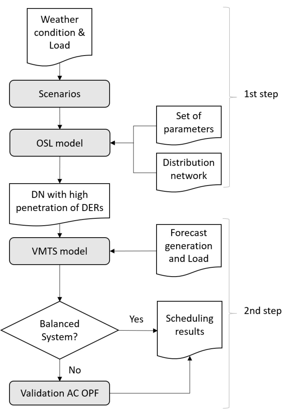
Figure 2.
Capacity and location of DERs in the PG&E 33-bus radial distribution network.
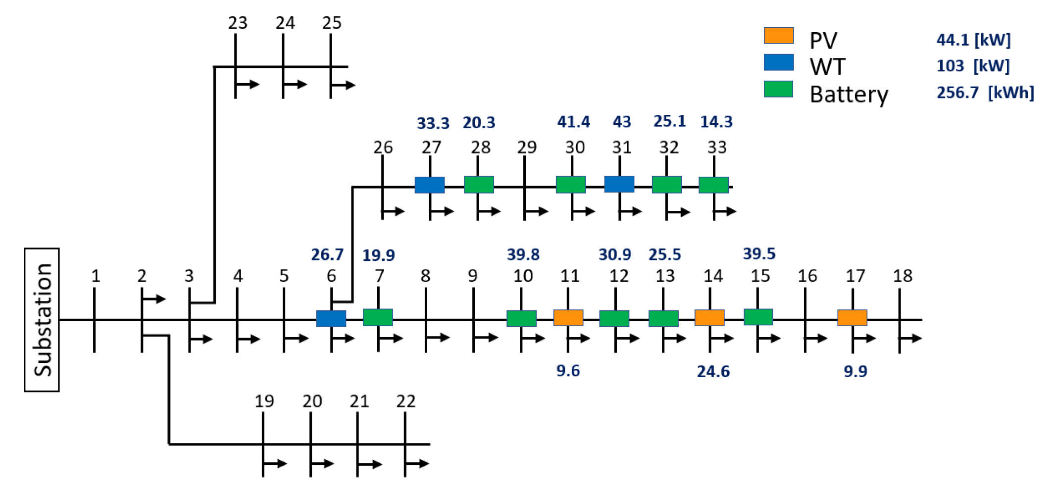
Figure 3.
The four consecutive scenarios of 72 h. The vertical axis is the percentage of the total capacity that can be used by the WT/PV or the percentage of the energy demand for every hour.
Figure 3.
The four consecutive scenarios of 72 h. The vertical axis is the percentage of the total capacity that can be used by the WT/PV or the percentage of the energy demand for every hour.

Figure 4.
Scenario 4: electricity demand fulfillment behavior.
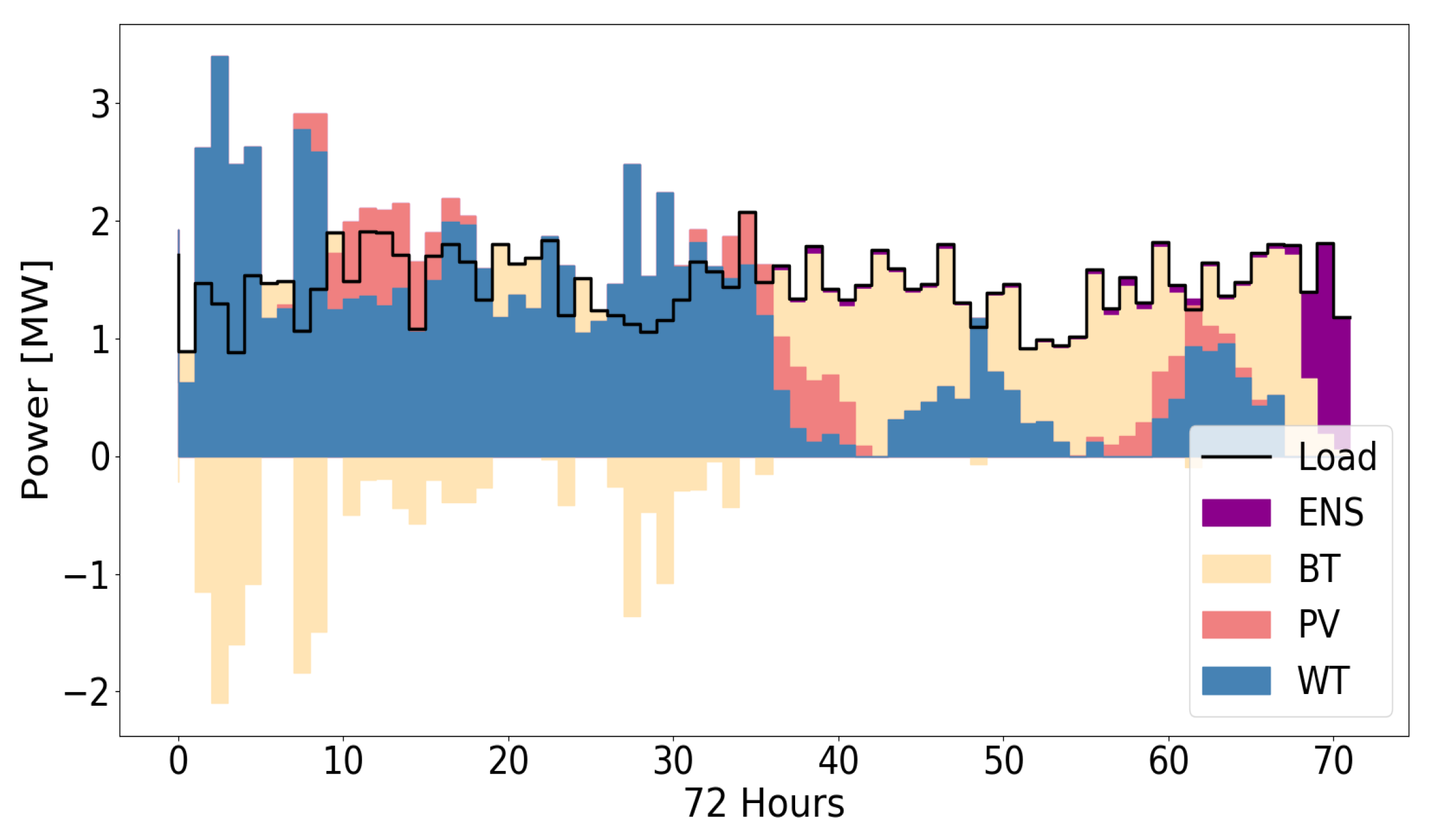
Figure 5.
Scenario 4: SOC of batteries vs. load, and wind/irradiance resources available.
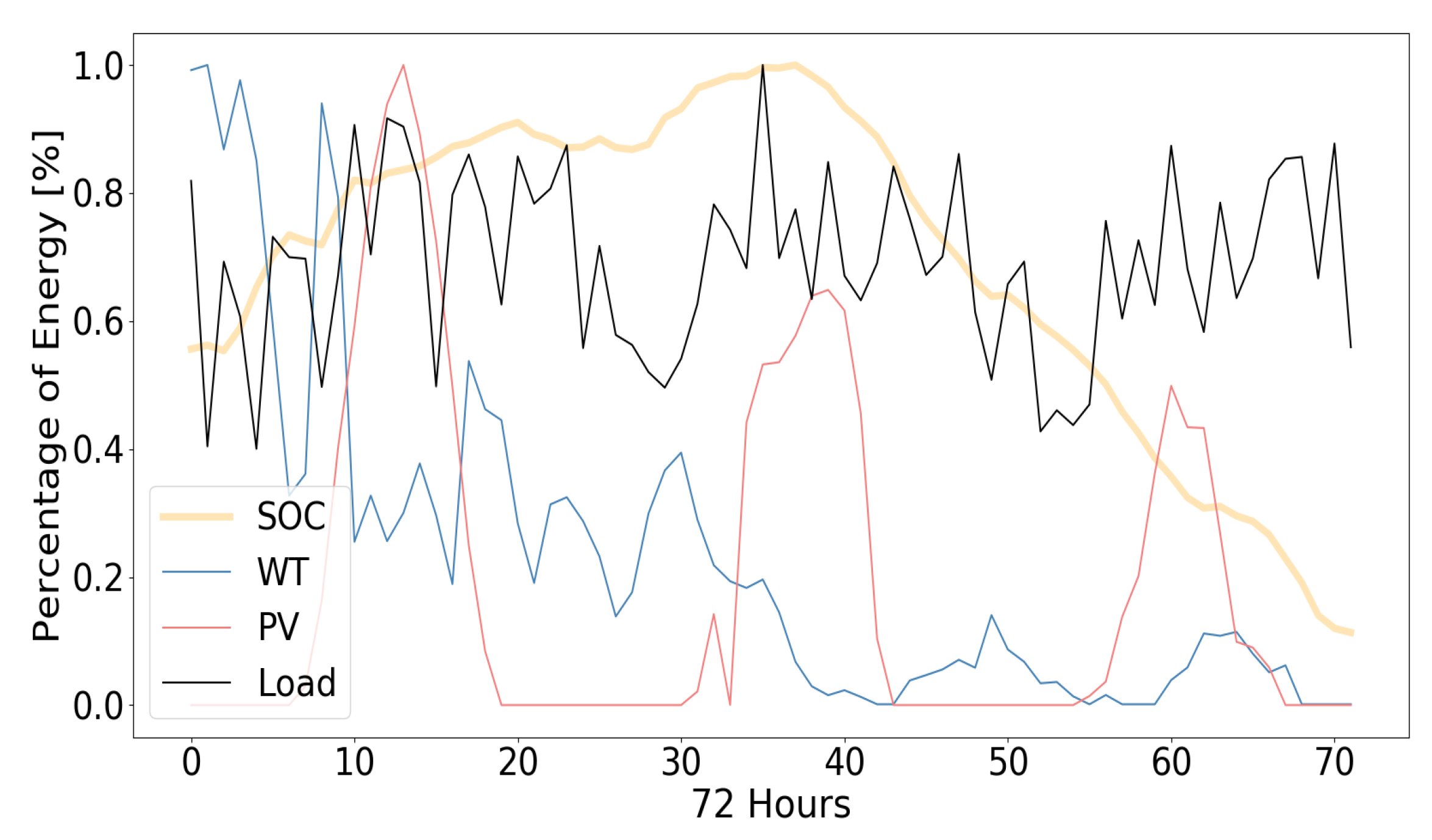
Figure 6.
PG&E 33-bus radial DN partitioning for the second scenario at 46 h. Red balls indicate the loads reduced to zero, without considering DSR in the model.
Figure 6.
PG&E 33-bus radial DN partitioning for the second scenario at 46 h. Red balls indicate the loads reduced to zero, without considering DSR in the model.
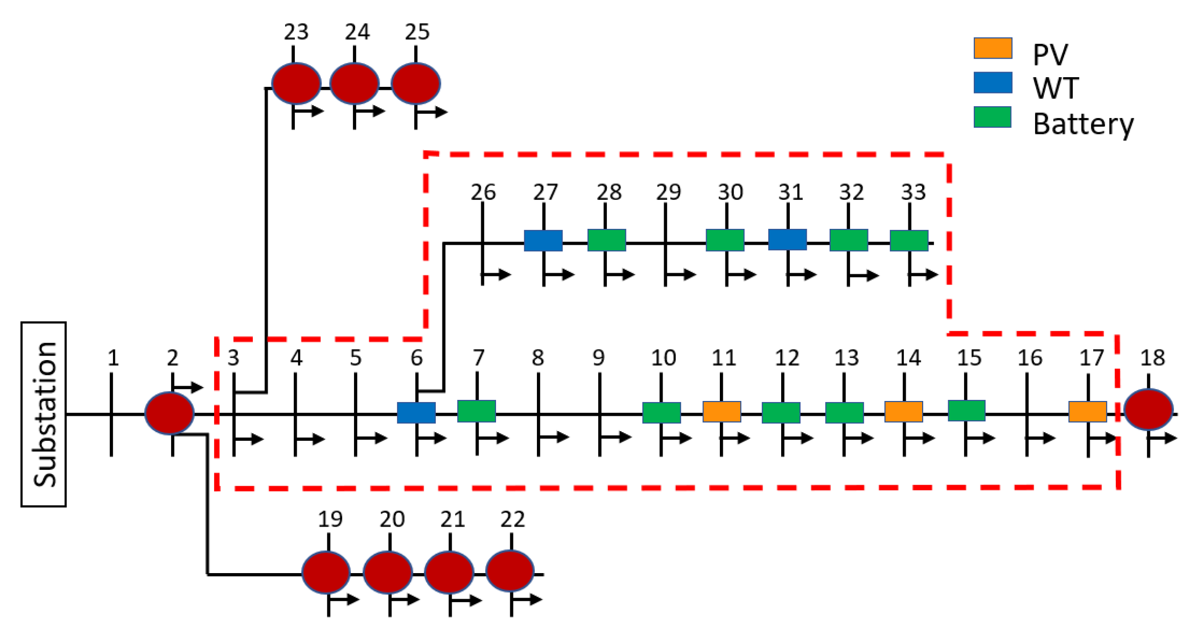
Figure 7.
PG&E 33-bus radial DN partitioning for the second scenario at 46 h, considering DSR in the model.
Figure 7.
PG&E 33-bus radial DN partitioning for the second scenario at 46 h, considering DSR in the model.


Table 1.
Performance of the MINLP and MILP.
| 1 h | 6 h | 12 h | 24 h | 72 h | |
|---|---|---|---|---|---|
| MINLP [s] | 1.79 | 25.86 | 20,038.7 | – | – |
| OF [kWh/pr.] | 0.1 | 0.65 | 1.32 | – | – |
| Status | ok | ok | ok | – | – |
| MILP [s] | 0.15 | 0.26 | 0.892 | 4.12 | 58.38 |
| OF [kWh/pr.] | 0.1 | 0.69 | 1.41 | 3.79 | 534,496.43 |
| Status | ok | ok | ok | ok | ok |
| OF error | 0% | 6.2% | 6.8% | – | – |
Table 2.
Probability that a bus has energy not supplied.
| Without DSR | With DSR | DERs Installed | |||||||||
|---|---|---|---|---|---|---|---|---|---|---|---|
| Bus | Sc 1 | Sc 2 | Sc 3 | Sc 4 | Total | Sc 1 | Sc 2 | Sc 3 | Sc 4 | Total | |
| 1 | 0.0% | 0.0% | 0.0% | 0.0% | 0.0% | 0.0% | 0.0% | 0.0% | 0.0% | 0.0% | No |
| 2 | 65.3% | 52.8% | 37.5% | 4.2% | 39.9% | 11.1% | 5.6% | 1.4% | 0.0% | 4.5% | No |
| 3 | 65.3% | 6.9% | 5.6% | 4.2% | 20.5% | 11.1% | 5.6% | 1.4% | 0.0% | 4.5% | No |
| 4 | 45.8% | 5.6% | 2.8% | 4.2% | 14.6% | 9.7% | 5.6% | 1.4% | 0.0% | 4.2% | No |
| 5 | 25.0% | 4.2% | 0.0% | 4.2% | 8.3% | 5.6% | 4.2% | 1.4% | 0.0% | 2.8% | Next, to WT |
| 6 | 8.3% | 2.8% | 0.0% | 4.2% | 3.8% | 0.0% | 2.8% | 0.0% | 0.0% | 0.7% | WT |
| 7 | 8.3% | 5.6% | 1.4% | 4.2% | 4.9% | 9.7% | 5.6% | 1.4% | 0.0% | 4.2% | BESS |
| 8 | 65.3% | 6.9% | 2.8% | 4.2% | 19.8% | 11.1% | 5.6% | 0.0% | 0.0% | 4.2% | Next, to BESS |
| 9 | 48.6% | 6.9% | 1.4% | 2.8% | 14.9% | 11.1% | 5.6% | 0.0% | 0.0% | 4.2% | Next, to BESS |
| 10 | 11.1% | 6.9% | 1.4% | 2.8% | 5.6% | 11.1% | 4.2% | 0.0% | 0.0% | 3.8% | BESS |
| 11 | 20.8% | 11.1% | 2.8% | 2.8% | 9.4% | 8.3% | 5.6% | 0.0% | 0.0% | 3.5% | PV |
| 12 | 12.5% | 13.9% | 5.6% | 2.8% | 8.7% | 12.5% | 5.6% | 0.0% | 0.0% | 4.5% | BESS |
| 13 | 13.9% | 13.9% | 2.8% | 2.8% | 8.3% | 12.5% | 2.8% | 0.0% | 0.0% | 3.8% | BESS |
| 14 | 43.1% | 9.7% | 5.6% | 2.8% | 15.3% | 9.7% | 2.8% | 2.8% | 0.0% | 3.8% | PV |
| 15 | 15.3% | 13.9% | 5.6% | 1.4% | 9.0% | 13.9% | 5.6% | 2.8% | 0.0% | 5.6% | BESS |
| 16 | 48.6% | 13.9% | 6.9% | 2.8% | 18.1% | 13.9% | 9.7% | 2.8% | 0.0% | 6.6% | Next, to PV |
| 17 | 70.8% | 13.9% | 5.6% | 2.8% | 23.3% | 12.5% | 5.6% | 2.8% | 0.0% | 5.2% | PV |
| 18 | 70.8% | 30.6% | 9.7% | 2.8% | 28.5% | 61.1% | 11.1% | 2.8% | 0.0% | 18.8% | Next, to PV |
| 19 | 66.7% | 66.7% | 50.0% | 4.2% | 46.9% | 51.4% | 5.6% | 1.4% | 0.0% | 14.6% | No |
| 20 | 68.1% | 90.3% | 72.2% | 4.2% | 58.7% | 63.9% | 6.9% | 1.4% | 0.0% | 18.1% | No |
| 21 | 69.4% | 100.0% | 79.2% | 15.3% | 66.0% | 65.3% | 54.2% | 2.8% | 0.0% | 30.6% | No |
| 22 | 69.4% | 100.0% | 79.2% | 47.2% | 74.0% | 65.3% | 62.5% | 2.8% | 0.0% | 32.6% | No |
| 23 | 65.3% | 58.3% | 43.1% | 4.2% | 42.7% | 26.4% | 5.6% | 1.4% | 0.0% | 8.3% | No |
| 24 | 68.1% | 76.4% | 59.7% | 4.2% | 52.1% | 58.3% | 6.9% | 1.4% | 0.0% | 16.7% | No |
| 25 | 68.1% | 100.0% | 79.2% | 4.2% | 62.8% | 65.3% | 6.9% | 2.8% | 0.0% | 18.8% | No |
| 26 | 4.2% | 2.8% | 0.0% | 4.2% | 2.8% | 0.0% | 1.4% | 0.0% | 0.0% | 0.3% | Next, to WT |
| 27 | 0.0% | 0.0% | 0.0% | 4.2% | 1.0% | 0.0% | 0.0% | 0.0% | 0.0% | 0.0% | WT |
| 28 | 5.6% | 4.2% | 0.0% | 2.8% | 3.1% | 4.2% | 2.8% | 1.4% | 0.0% | 2.1% | BESS |
| 29 | 6.9% | 4.2% | 0.0% | 2.8% | 3.5% | 8.3% | 4.2% | 1.4% | 0.0% | 3.5% | Next, to BESS |
| 30 | 5.6% | 4.2% | 0.0% | 2.8% | 3.1% | 6.9% | 2.8% | 0.0% | 0.0% | 2.4% | BESS |
| 31 | 0.0% | 1.4% | 0.0% | 2.8% | 1.0% | 0.0% | 0.0% | 0.0% | 0.0% | 0.0% | WT |
| 32 | 6.9% | 4.2% | 1.4% | 2.8% | 3.8% | 8.3% | 1.4% | 0.0% | 0.0% | 2.4% | BESS |
| 33 | 8.3% | 4.2% | 1.4% | 1.4% | 3.8% | 9.7% | 4.2% | 1.4% | 0.0% | 3.8% | BESS |
Table 3.
Energy not supplied and its percentage of non-compliance.
| Without DSR | With DSR | DERs Installed | |||||||||||||||
|---|---|---|---|---|---|---|---|---|---|---|---|---|---|---|---|---|---|
| ENS [MWh] | ENS % | ENS [MWh] | ENS % | ||||||||||||||
| Bus | Sc 1 | Sc 2 | Sc 3 | Sc 4 | Sc 1 | Sc 2 | Sc 3 | Sc 4 | Sc 1 | Sc 2 | Sc 3 | Sc 4 | Sc 1 | Sc 2 | Sc 3 | Sc 4 | |
| 1 | 0 | 0 | 0 | 0 | 0% | 0% | 0% | 0% | 0 | 0 | 0 | 0 | 0% | 0% | 0% | 0% | No |
| 2 | 2.3 | 1.4 | 1.1 | 0.1 | 66% | 54% | 36% | 4% | 0.3 | 0.1 | 0 | 0 | 8% | 4% | 1% | 0% | No |
| 3 | 2.1 | 0.2 | 0.1 | 0.1 | 66% | 8% | 5% | 4% | 0.3 | 0.1 | 0 | 0 | 8% | 4% | 1% | 0% | No |
| 4 | 1.8 | 0.2 | 0.1 | 0.1 | 43% | 6% | 3% | 4% | 0.3 | 0.1 | 0 | 0 | 7% | 4% | 1% | 0% | No |
| 5 | 0.3 | 0.1 | 0 | 0.1 | 16% | 4% | 0% | 4% | 0.1 | 0 | 0 | 0 | 3% | 2% | 1% | 0% | Next, to WT |
| 6 | 0.1 | 0 | 0 | 0.1 | 5% | 2% | 0% | 4% | 0 | 0 | 0 | 0 | 0% | 1% | 0% | 0% | WT |
| 7 | 0.5 | 0.2 | 0 | 0.2 | 8% | 5% | 0% | 4% | 0.3 | 0.2 | 0 | 0 | 5% | 3% | 0% | 0% | BESS |
| 8 | 4.6 | 0.3 | 0.1 | 0.2 | 66% | 6% | 2% | 3% | 0.6 | 0.2 | 0 | 0 | 8% | 4% | 0% | 0% | Next, to BESS |
| 9 | 1 | 0.1 | 0 | 0.1 | 49% | 8% | 2% | 3% | 0.2 | 0.1 | 0 | 0 | 8% | 4% | 0% | 0% | Next, to BESS |
| 10 | 0.2 | 0.1 | 0 | 0.1 | 10% | 8% | 2% | 3% | 0.2 | 0.1 | 0 | 0 | 7% | 3% | 0% | 0% | BESS |
| 11 | 0.3 | 0.1 | 0 | 0 | 17% | 9% | 2% | 3% | 0.1 | 0 | 0 | 0 | 6% | 2% | 0% | 0% | PV |
| 12 | 0.3 | 0.2 | 0.1 | 0.1 | 12% | 15% | 5% | 3% | 0.2 | 0.1 | 0 | 0 | 8% | 4% | 0% | 0% | BESS |
| 13 | 0.3 | 0.2 | 0 | 0.1 | 13% | 13% | 2% | 3% | 0.2 | 0 | 0 | 0 | 9% | 1% | 0% | 0% | BESS |
| 14 | 1.5 | 0.2 | 0.2 | 0 | 35% | 7% | 4% | 1% | 0.2 | 0 | 0 | 0 | 6% | 0% | 1% | 0% | PV |
| 15 | 0.3 | 0.2 | 0.1 | 0 | 14% | 14% | 5% | 1% | 0.2 | 0.1 | 0 | 0 | 8% | 4% | 1% | 0% | BESS |
| 16 | 1 | 0.2 | 0.1 | 0.1 | 46% | 15% | 6% | 3% | 0.2 | 0.1 | 0 | 0 | 10% | 7% | 2% | 0% | Next, to PV |
| 17 | 1.2 | 0.1 | 0.1 | 0.1 | 58% | 9% | 5% | 3% | 0.2 | 0.1 | 0 | 0 | 7% | 4% | 2% | 0% | PV |
| 18 | 2.2 | 0.7 | 0.2 | 0.1 | 71% | 29% | 8% | 3% | 1.4 | 0.2 | 0.1 | 0 | 43% | 8% | 2% | 0% | Next, to PV |
| 19 | 2.1 | 1.5 | 1.2 | 0.1 | 67% | 67% | 46% | 4% | 1.2 | 0.1 | 0 | 0 | 38% | 4% | 1% | 0% | No |
| 20 | 2.2 | 2.1 | 1.9 | 0.1 | 68% | 92% | 69% | 4% | 1.4 | 0.1 | 0 | 0 | 45% | 5% | 1% | 0% | No |
| 21 | 2.2 | 2.3 | 2.1 | 0.4 | 69% | 100% | 77% | 15% | 1.5 | 0.9 | 0.1 | 0 | 46% | 38% | 2% | 0% | No |
| 22 | 2.2 | 2.3 | 2.1 | 1.1 | 69% | 100% | 77% | 47% | 1.5 | 1 | 0.1 | 0 | 46% | 45% | 2% | 0% | No |
| 23 | 2.1 | 1.3 | 1.1 | 0.1 | 66% | 59% | 40% | 4% | 0.5 | 0.1 | 0 | 0 | 17% | 4% | 1% | 0% | No |
| 24 | 9.9 | 7.9 | 6.6 | 0.5 | 67% | 75% | 53% | 4% | 6.1 | 0.5 | 0.1 | 0 | 42% | 5% | 1% | 0% | No |
| 25 | 10 | 10.5 | 9.4 | 0.5 | 68% | 99% | 75% | 4% | 6.7 | 0.6 | 0.2 | 0 | 46% | 5% | 2% | 0% | No |
| 26 | 0 | 0 | 0 | 0.1 | 1% | 2% | 0% | 4% | 0 | 0 | 0 | 0 | 0% | 1% | 0% | 0% | Next, to WT |
| 27 | 0 | 0 | 0 | 0.1 | 0% | 0% | 0% | 4% | 0 | 0 | 0 | 0 | 0% | 0% | 0% | 0% | WT |
| 28 | 0.1 | 0.1 | 0 | 0.1 | 4% | 3% | 0% | 3% | 0 | 0 | 0 | 0 | 2% | 2% | 1% | 0% | BESS |
| 29 | 0.3 | 0.1 | 0 | 0.1 | 7% | 4% | 0% | 3% | 0.2 | 0.1 | 0 | 0 | 4% | 3% | 1% | 0% | Next, to BESS |
| 30 | 0.4 | 0.1 | 0 | 0.2 | 5% | 3% | 0% | 3% | 0.3 | 0 | 0 | 0 | 4% | 1% | 0% | 0% | BESS |
| 31 | 0 | 0 | 0 | 0.1 | 0% | 0% | 0% | 3% | 0 | 0 | 0 | 0 | 0% | 0% | 0% | 0% | WT |
| 32 | 0.4 | 0.1 | 0 | 0.1 | 5% | 2% | 0% | 2% | 0.2 | 0.1 | 0 | 0 | 2% | 1% | 0% | 0% | BESS |
| 33 | 0.2 | 0.1 | 0 | 0 | 8% | 4% | 2% | 1% | 0.1 | 0.1 | 0 | 0 | 6% | 3% | 0% | 0% | BESS |
Table 4.
DN topology under the second scenario.
| Scenario 2 without DSR | Scenario 2 with DSR | |||||||||||||||||
|---|---|---|---|---|---|---|---|---|---|---|---|---|---|---|---|---|---|---|
| Bus | 40 | 41 | 42 | 43 | 44 | 45 | 46 | 47 | 48 | 40 | 41 | 42 | 43 | 44 | 45 | 46 | 47 | 48 |
| 1 | 0 | 0 | 0 | 0 | 0 | 0 | 0 | 0 | 0 | 0 | 0 | 0 | 0 | 0 | 0 | 0 | 0 | 0 |
| 2 | 0 | 0 | 0 | 0 | 1 | 1 | 1 | 1 | 1 | 0 | 0 | 0 | 0 | 0 | 0 | 0 | 0 | 0 |
| 3 | 0 | 0 | 0 | 0 | 0 | 0 | 0 | 0 | 0 | 0 | 0 | 0 | 0 | 0 | 0 | 0 | 0 | 0 |
| 4 | 0 | 0 | 0 | 0 | 0 | 0 | 0 | 0 | 0 | 0 | 0 | 0 | 0 | 0 | 0 | 0 | 0 | 0 |
| 5 | 0 | 0 | 0 | 0 | 0 | 0 | 0 | 0 | 0 | 0 | 0 | 0 | 0 | 0 | 0 | 0 | 0 | 0 |
| 6 | 0 | 0 | 0 | 0 | 0 | 0 | 0 | 0 | 0 | 0 | 0 | 0 | 0 | 0 | 0 | 0 | 0 | 0 |
| 7 | 0 | 0 | 0 | 0 | 0 | 0 | 0 | 0 | 0 | 0 | 0 | 0 | 0 | 0 | 0 | 0 | 0 | 0 |
| 8 | 0 | 0 | 0 | 0 | 0 | 0 | 0 | 0 | 0 | 0 | 0 | 0 | 0 | 0 | 0 | 0 | 0 | 0 |
| 9 | 0 | 0 | 0 | 0 | 0 | 0 | 0 | 0 | 0 | 0 | 0 | 0 | 0 | 0 | 0 | 0 | 0 | 0 |
| 10 | 0 | 0 | 0 | 0 | 0 | 0 | 0 | 0 | 0 | 0 | 0 | 0 | 0 | 0 | 0 | 0 | 0 | 0 |
| 11 | 0 | 0 | 0 | 0 | 0 | 0 | 0 | 0 | 0 | 0 | 0 | 0 | 0 | 0 | 0 | 0 | 0 | 0 |
| 12 | 0 | 0 | 0 | 0 | 0 | 0 | 0 | 0 | 0 | 0 | 0 | 0 | 0 | 0 | 0 | 0 | 0 | 0 |
| 13 | 0 | 0 | 0 | 0 | 0 | 0 | 0 | 0 | 0 | 0 | 0 | 0 | 0 | 0 | 0 | 0 | 0 | 0 |
| 14 | 0 | 0 | 0 | 0 | 0 | 0 | 0 | 0 | 0 | 0 | 0 | 0 | 0 | 0 | 0 | 0 | 0 | 0 |
| 15 | 0 | 0 | 0 | 0 | 0 | 0 | 0 | 0 | 0 | 0 | 0 | 0 | 0 | 0 | 0 | 0 | 0 | 0 |
| 16 | 0 | 0 | 0 | 0 | 0 | 0 | 0 | 0 | 0 | 0 | 0 | 0 | 0 | 0 | 0 | 0 | 0 | 0 |
| 17 | 0 | 0 | 0 | 0 | 0 | 0 | 0 | 0 | 0 | 0 | 0 | 0 | 0 | 0 | 0 | 0 | 0 | 0 |
| 18 | 0 | 0 | 1 | 0 | 0 | 0 | 1 | 0 | 0 | 0 | 0 | 0 | 0 | 0 | 0 | 0 | 0 | 0 |
| 19 | 0 | 0 | 0 | 0 | 1 | 1 | 1 | 1 | 1 | 0 | 0 | 0 | 0 | 0 | 0 | 0 | 0 | 0 |
| 20 | 1 | 1 | 1 | 1 | 1 | 1 | 1 | 1 | 1 | 0 | 0 | 0 | 0 | 0 | 0 | 0 | 0 | 0 |
| 21 | 1 | 1 | 1 | 1 | 1 | 1 | 1 | 1 | 1 | 0 | 0 | 0 | 0 | 1 | 1 | 1 | 1 | 1 |
| 22 | 1 | 1 | 1 | 1 | 1 | 1 | 1 | 1 | 1 | 0 | 0 | 0 | 0 | 1 | 1 | 1 | 1 | 1 |
| 23 | 0 | 0 | 0 | 0 | 1 | 1 | 1 | 1 | 1 | 0 | 0 | 0 | 0 | 0 | 0 | 0 | 0 | 0 |
| 24 | 1 | 0 | 1 | 1 | 1 | 1 | 1 | 1 | 1 | 0 | 0 | 0 | 0 | 0 | 0 | 0 | 0 | 0 |
| 25 | 1 | 1 | 1 | 1 | 1 | 1 | 1 | 1 | 1 | 0 | 0 | 0 | 0 | 0 | 0 | 0 | 0 | 0 |
| 26 | 0 | 0 | 0 | 0 | 0 | 0 | 0 | 0 | 0 | 0 | 0 | 0 | 0 | 0 | 0 | 0 | 0 | 0 |
| 27 | 0 | 0 | 0 | 0 | 0 | 0 | 0 | 0 | 0 | 0 | 0 | 0 | 0 | 0 | 0 | 0 | 0 | 0 |
| 28 | 0 | 0 | 0 | 0 | 0 | 0 | 0 | 0 | 0 | 0 | 0 | 0 | 0 | 0 | 0 | 0 | 0 | 0 |
| 29 | 0 | 0 | 0 | 0 | 0 | 0 | 0 | 0 | 0 | 0 | 0 | 0 | 0 | 0 | 0 | 0 | 0 | 0 |
| 30 | 0 | 0 | 0 | 0 | 0 | 0 | 0 | 0 | 0 | 0 | 0 | 0 | 0 | 0 | 0 | 0 | 0 | 0 |
| 31 | 0 | 0 | 0 | 0 | 0 | 0 | 0 | 0 | 0 | 0 | 0 | 0 | 0 | 0 | 0 | 0 | 0 | 0 |
| 32 | 0 | 0 | 0 | 0 | 0 | 0 | 0 | 0 | 0 | 0 | 0 | 0 | 0 | 0 | 0 | 0 | 0 | 0 |
| 33 | 0 | 0 | 0 | 0 | 0 | 0 | 0 | 0 | 0 | 0 | 0 | 0 | 0 | 0 | 0 | 0 | 0 | 0 |
Publisher’s Note: MDPI stays neutral with regard to jurisdictional claims in published maps and institutional affiliations. |
© 2020 by the authors. Licensee MDPI, Basel, Switzerland. This article is an open access article distributed under the terms and conditions of the Creative Commons Attribution (CC BY) license (http://creativecommons.org/licenses/by/4.0/).
Share and Cite
MDPI and ACS Style
García-Muñoz, F.; Díaz-González, F.; Corchero, C. A Mathematical Model for the Scheduling of Virtual Microgrids Topology into an Active Distribution Network. Appl. Sci. 2020, 10, 7199. https://doi.org/10.3390/app10207199
AMA Style
García-Muñoz F, Díaz-González F, Corchero C. A Mathematical Model for the Scheduling of Virtual Microgrids Topology into an Active Distribution Network. Applied Sciences. 2020; 10(20):7199. https://doi.org/10.3390/app10207199
Chicago/Turabian StyleGarcía-Muñoz, Fernando, Francisco Díaz-González, and Cristina Corchero. 2020. "A Mathematical Model for the Scheduling of Virtual Microgrids Topology into an Active Distribution Network" Applied Sciences 10, no. 20: 7199. https://doi.org/10.3390/app10207199
Note that from the first issue of 2016, this journal uses article numbers instead of page numbers. See further details here.