Correction of Young’s Modulus Calculation in the Flexural Mode of Resonant Column Test

Abstract

The resonant column test includes torsional and flexural modes that can be used to obtain reduction curves for the shear modulus and Young’s modulus of the soil, respectively. When the resonant column test is performed under flexural mode, Young’s modulus is calculated mainly using the measured resonant frequency following the formula proposed by Cascante et al. However, this formula does not consider the rotational inertia effect of the electromagnetic drive disk of the resonant column apparatus and thus may inaccurately calculate Young’s modulus. In this study, the formula was modified by considering the rotational inertia effect of the electromagnetic drive disk, and its accuracy was verified by using three aluminum calibration rods with different diameters as a dummy specimen for the resonant tests in flexural and torsional modes.

1. Introduction

Soil dynamic properties (including shear modulus G and Young’s modulus E) and damping ratio are indispensable parameters in the dynamic analysis of ground responses or foundation structures subjected to earthquake motions. In situ tests, such as the spectral analysis of surface waves, down-hole method, or cross-hole method, are typically used to measure the shear and compression wave velocities of the soil layer, which are then converted to the dynamic properties of soil (e.g., G and E) under small strain. However, the dynamic characteristics of soil under different strains (i.e., shear modulus reduction curve and damping curve) are primarily measured by laboratory tests, such as dynamic triaxial, cyclic simple shear, resonant column, shaking table, and centrifuge modeling.

The resonant column test, including torsional and flexural modes (Figure 1), is commonly used to measure the resonant frequencies of specimens to obtain soil dynamic properties. High-frequency torsional or flexural vibrations are applied to the specimen by electromagnetic drive discs (EDDs), and the torsional/flexural resonant frequencies are detected at the corresponding strain. On the basis of the measured resonant frequency, the G or E of the soil is determined using the calculation formula. In general, torsional mode is commonly used because G and its reduction curve are indispensable properties in the site response analysis for propagating horizontal ground motions [1,2]. With the demand for the assessment of vertical ground movement under earthquake, E or constrained modulus and its reduction curve have become increasingly important [3,4,5].

The formulas proposed by Cascante et al. [6] and documented in ASTM D4015 [7] can be used to calculate the G and E of the soil with torsional and flexural resonant frequencies, respectively. The torsional inertia of the EDD is considered in the calculation formula for torsional vibration mode to ensure the accurate evaluation of G. Later studies further examined the counter electromotive effect [8,9] and equipment effects [10,11] on the measurement of stiffness and damping in soils. However, these studies focused on the effect in torsional vibration mode and the improvements to the calibration in flexural vibration mode are limited. The calculation formula of flexural vibration in [6] only considers the mass inertia of the EDD but does not include the rotational inertia, thus possibly leading to inaccurate assessment for E. Therefore, this study considers the rotational inertia effect of the EDD and corrects the formula of Cascante et al. [6] for the E calculation. The accuracy of the modified formula is verified through the testing of an aluminum calibration rod with known E, G, and Poisson’s ratio (ν).

2. Analysis Method of Flexural Test

2.1. Calibration of Flexural Test

E was theoretically calculated from the flexural test following the formula by Cascante et al. [6]. During the flexural vibration, the effect of the inertia of driving systems on the resonant frequency cannot be directly assessed because of the complex EDD structure of the resonant column apparatus (Figure 2). Prior to using the calculation formula, the inertia effect of the EDD must first be calibrated to accurately compute for the E of the specimen.

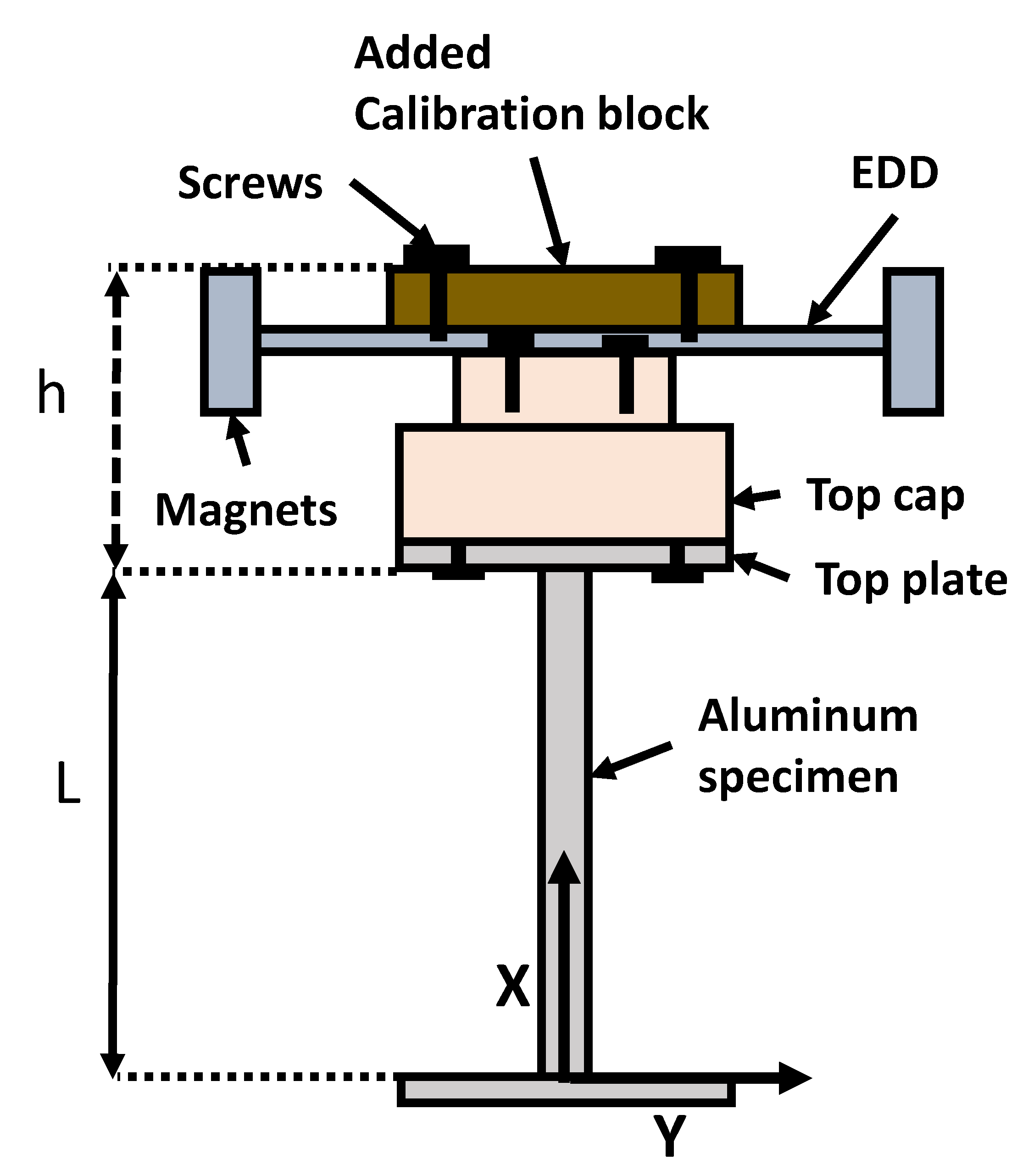
The configuration of the calibration test is shown in Figure 3. An aluminum calibration rod (a dummy specimen) is locked on the base and EDD through the top cap. Calibration for the EDD and calculation of E are conducted as follows:

• The flexural resonant frequency f1 is measured for the condition with an aluminum calibration rod through the flexural resonant test.
• A calibration block with known mass is added to the EDD, and the flexural resonant frequency f2 is measured after the plate is added.
• The inertial effect of the EDD is assessed using f1 and f2.
• The E of the calibration rod is calculated according to f1 while accounting for the inertial effect of the EDD in Step 3.

Figure 3 shows that the rotational inertia of the EDD during the flexural vibration has greater influence on the flexural vibration frequency because its radius is larger than that of other accessories. This condition must be considered in amending the calculation formula.

2.2. Inertial Effect and Calibration of Electromagnetic Drive Disk

Cascante et al. [6] used the Rayleigh method to analyze the resonant frequency in the flexural mode. The deformation of the calibration rod can be regarded as a cantilever beam in the flexural resonant test. The EDD centroid is achieved when the maximum strain energy is equal to the kinetic energy.

As shown in Figure 3, the calibration rod is divided into three parts for the analysis: The bottom plate (regarded as the fixed end at the bottom), the middle section with length L, and the top plate. The horizontal deformation (y) of the rod at different elevations (x) is assumed to be a third-order polynomial:

$$\mathrm{y}\left(\mathrm{x}\right)=a_0+a_{1}x+a_2{x}^2+a_3{x}^3$$

(1)

Given that the bottom of the rod (x = 0) is fixed on the base, its displacement $\mathrm{y}\left(0\right)=0$ and slope ${\mathrm{y}}^{\prime }\left(0\right)=0$, and coefficients $a_0 \mathrm{and} a_1$ are zero. In addition, the top of the rod (x = L) is a free end, and its bending moment is $\mathrm{EI}{y}^{″}\left(L\right)=0$. Hence, Equation (1) can be rewritten as:

$$\mathrm{y}\left(\mathrm{x}\right)=\mathsf{\alpha }{x}^2\left[3L-x\right] for x<L$$

(2)

where $\mathsf{\alpha }=\left(a_2/3L\right)$. Equation (2) is the deformation equation applied to the middle section of the rod (excluding top plate and bottom plate of the calibration rod). The top plate, EDD, and calibration block can be regarded as the rigid body added to the top of the rod. Hence, their displacement can be expressed in terms of the displacement $\mathrm{y}\left(L\right)$ and slope ${\mathrm{y}}^{\prime }\left(L\right)$ of the top of the rod:

$$\mathrm{y}\left(\mathrm{x}\right)=\mathsf{\alpha }{L}^2\left[2L+3\left(x-L\right)\right] for x>L$$

(3)

The maximum displacement of the rod occurs at the resonant frequency, and the maximum strain energy of the rod is calculated as

$$J_U=\frac{1}{2}E{I}_b{{\displaystyle \int }}_0^L{y}^{″}{\left(x\right)}^{2}dx=6E{I}_b{\alpha }^2{L}^3$$

(4)

where $I_b$ is the moment of inertia of the rod. The rod vibrating back and forth at a fixed frequency (e.g., resonant frequency) can be regarded as a simple harmonic motion with the angular frequency ${\omega }_f$. As a result, maximum kinetic energy $J_{T1}$ can be calculated as

$$J_{T1}=\frac{1}{2}{{\omega }_f}^{2}A{{\displaystyle \int }}_0^{6}y{\left(x\right)}^{2}dx=\frac{33}{70}{{\omega }_f}^2{\alpha }^2{L}^6{m}_T$$

(5)

where A is the cross-sectional area of the rod and $m_T$ is the mass of the rod. The kinetic energy of the rigid body with mass ($m$) above the top of the rod is calculated according to the distance of its centroid from the top of rod h:

$$J_{T2}=\frac{1}{2}m{\left[\alpha L^2\left(2L+3h\right)\right]}^2·{{\omega }_f}^2=\mathrm{m}{\alpha }^2{L}^6\left[2+6\frac{h}{L}+\frac{9}{2}{\left(\frac{h}{L}\right)}^2\right]·{{\omega }_f}^2$$

(6)

The resonant frequency of the system from the flexural resonant test can be obtained when the kinetic energy of the system ($J_{T1}+J_{T2})$ is equal to the strain energy of the rod ($J_U)$ according to the conservation of energy:

$${\omega }_f=\frac{3E{I}_b}{\left\{\frac{33}{140}{m}_T+m\left[1+3\frac{h}{L}+\frac{9}{4}{\left(\frac{h}{L}\right)}^2\right]\right\}·L^3}$$

(7)

In Equation (7), the effect of the kinetic energy of the rigid bodies above the top of the rod on the measured frequency can be expressed as the product of their mass and the height of the centroid. Hence, this formula can be rewritten as:

$${\omega }_f=\frac{3E{I}_b}{\left[\frac{33}{140}{m}_T+{{\displaystyle \sum }}_{i=0}^N{m}_i·h\left(h{0}_i,h{1}_i\right)\right]·L^3}$$

(8)

where $m_i$ is the mass of the individual rigid body above the top of the rod; and $h{0}_i$ and $h{1}_i$ are the heights from the bottom and top of the individual rigid body to the top of the rod, respectively. If the centroid is $\left(h{0}_i+h{1}_i\right)/2$, then the function of centroid $h\left(h{0}_i,h{1}_i\right)$ in respect to the top of the rod in Equation (7) is rewritten as:

$$h\left(h{0}_i,h{1}_i\right)=1+\frac{3\left(h{0}_i+h{1}_i\right)}{2L}+\frac{9}{16}·\left(\frac{{h{0}_i}^2+2h{0}_{i}h{1}_i+{h{1}_i}^2}{L^2}\right)$$

(9)

The coefficient of the last term of Equation (9) ($9/16$) differs from that of the formula derived by Cascante et al. [6] ($3/4$) and is therefore used to compare and analyze the results. Except for the EDD, the rest of the components (i.e., the top plate, top cap, and calibration block) have fixed cross-sections, and their centroids can be calculated directly. However, the centroid of the EDD with an irregular cross-section must be obtained using Equation (8) through to the inverse calculation of the flexural resonant frequency as described in Section 2.1. and Section 2.3. After the position of the centroid of the EDD is determined, the E of the rod or specimen can be calculated based on the measured resonant frequency (Equation (8)).

2.3. Correction for the Rotational Effect of EDD

The proposed formula for the flexural mode (Equation (8)) does not consider the influence of the rotational inertia of the EDD and the top cap on the resonant frequency. Owing to its considerable radius and mass, the rotational influence of the EDD must be considered to improve the accuracy of Young’s modulus estimation.

According to the displacement equation of the specimen (Equation (2)), the rotation angle at the top of the specimen ($∆\mathsf{\theta }$) is calculated as:

$$∆\mathsf{\theta }=3\mathsf{\alpha }{L}^2$$

(10)

The average angular velocity ($\overline{\omega }$) of the top cap and the EDD can be obtained using the rotation angle and the vibration frequency (f) of the specimen at resonance. The conversion between average angular velocity $\overline{\omega }$ and resonant frequency ${\omega }_f$ is shown in Equation (11):

$$\overline{\omega }=4∆\theta \times f=\frac{4∆\theta }{2\pi }\times {\omega }_f=\frac{6\alpha L^2}{\pi }\times {\omega }_f$$

(11)

When the specimen vibrates at the resonant frequency, rotational kinetic energy $J_{T3}$ of the top cap and the EDD can be computed as:

$$J_{T3}=\frac{1}{2}\times I_T\times {(\frac{6\alpha L^2}{\pi }\times {\omega }_f)}^2$$

(12)

where $I_T$ is the rotational inertia of the top plate, top cap, or EDD. According to the conservation of the energy state, the kinetic energy of the system $(J_{T1}+J_{T2}+J_{T3})$ is equal to the strain energy of the rod ($J_U)$. Therefore, Equation (8) is modified as:

$${{\omega }_f}^2=\frac{3E{I}_b}{\left\{\frac{33}{140}{m}_T+{{\displaystyle \sum }}_{i=0}^N{m}_i·h\left(h{0}_i,h{1}_i\right)+{{\displaystyle \sum }}_{i=0}^N{\left(\frac{3}{\pi L}\right)}^2{I}_{Ti}\right\}·L^3}$$

(13)

The mass of each component is substituted into Equation (13) to obtain:

$${{\omega }_1}^2=\frac{3E{I}_b}{\left\{\frac{33}{140}{m}_T+{\overline{m}}_a+{\overline{m}}_c+{\overline{m}}_d+{\overline{I}}_{T1}\right\}·L^3}$$

(14)

where ${\omega }_1$ is the flexural resonant frequency of the system with the calibration rod only; $m_T$ is the mass of the rod; ${\overline{m}}_a, {\overline{m}}_c, \mathrm{and} {\overline{m}}_d$ are the products of the mass and the centroid height of the top plate, top cap, and EDD, respectively; and ${\overline{I}}_{T1}$ is the sum of the product of the rotational inertia of the top plate, top cap, and EDD and its coefficient ${\left(\frac{3}{\pi L}\right)}^2$.

2.4. Corrected Calibration Formula of Flexural Test

Owing to the complex cross-section of the EDD, the product of its mass and the centroid of mass ${\overline{m}}_d$ and the sum of the moments of inertia ${\overline{I}}_{T1}$ cannot be directly obtained. A calibration block with a known mass added to the calibration rod is required to indirectly estimate ${\overline{m}}_d$ and ${\overline{I}}_{T1}$. After the flexural resonant frequency is measured under this condition (${\omega }_2$), substituting the mass property and resonant frequency into Equation (13) yields:

$${{\omega }_2}^2=\frac{3E{I}_b}{\left\{\frac{33}{140}{m}_T+{\overline{m}}_a+{\overline{m}}_c+{\overline{m}}_d+{\overline{m}}_{am}+{\overline{I}}_{T2}\right\}·L^3}=\frac{3E{I}_b}{\left\{\frac{33}{140}{m}_T+{\overline{m}}_a+{\overline{m}}_c+{\overline{m}}_d+{\overline{m}}_{am}+{\overline{I}}_{T1}+I_{am}\right\}·L^3}$$

(15)

where ${\overline{m}}_{am}$ is the product of the mass of the calibration block and its centroid height; ${\overline{I}}_{T2}$ is the total rotational inertia of the top plate, top cap, EDD, and calibration block; and $I_{am}$ is the rotational inertia of the calibration block. The calibration block is aligned with an angle of 45° in respect to the vibration direction to avoid the interruption with the wire and measuring instruments. Hence, the moment of inertia of the calibration block $I_{am}$ is calculated as follows:

$$I_{am}=\frac{I_y+I_z}{2}+\frac{I_y-I_z}{2}\cos 2\vartheta -I_{yz}\sin 2\vartheta$$

(16)

where $I_y$ and $I_z$ are the rotational inertia of the calibration block parallel and perpendicular to the vibration direction, respectively, and ϑ is the angle with respect to the vibration direction. The product of the mass of the EDD and its centroid and the summation of the moment of inertia (${\overline{I}}_{T1}$) can be obtained by combining Equations (14) and (15):

$${\overline{m}}_d+{\overline{I}}_{T1}=\frac{{{\omega }_2}^2\left({\overline{m}}_{am}+I_{am}\right)-\left({{\omega }_1}^2-{{\omega }_2}^2\right)\left(\frac{33}{140}{m}_T+{\overline{m}}_a+{\overline{m}}_c\right)}{{{\omega }_1}^2-{{\omega }_2}^2}={\overline{m}}_d+{\overline{I}}_d+{\overline{I}}_a+{\overline{I}}_c$$

(17)

where ${\overline{I}}_d$ is the product of the rotational inertia of EDD, and constants ${\left(\frac{3}{\pi L}\right)}^2$, and ${\overline{I}}_a$ and ${\overline{I}}_c$ are the products of the rotational inertia of the top plate and top cap and constant ${\left(\frac{3}{\pi L}\right)}^2$, respectively, which can be calculated according to Equation (18):

$$I=\frac{1}{4}m{r}^2$$

(18)

where r is the radius of the top plate/cap. The mass of the EDD can be measured, but the calculation for the centroid and moment of inertia is complicated. In addition, ${\overline{m}}_d$ and ${\overline{I}}_d$ are also functions of mass. Therefore, the centroid function and the rotational inertia function are integrated into an equal centroid for subsequent calculations as expressed in the following formula:

$${\overline{m}}_d+{\overline{I}}_d=m_d\times f\left(h\right)+m_d\times f\left(r\right)=m_d\times \left(f\left(h\right)+f\left(r\right)\right)=m_d\times h_d$$

(19)

where $m_d$ is the mass of the EDD, $f\left(h\right)$ is the centroid function of the EDD, $f\left(r\right)$ is the rotational inertia function of the EDD, and $h_d$ is the equivalent centroid position of the EDD accounting for the mass inertia and rotational inertia.

When $h_d$ is determined by Equation (17), it is replaced with (14) to calculate the E of the calibration rod or specimen:

$$E=\frac{{{\omega }_1}^2{L}^3\left(\frac{33}{140}{m}_T+{\overline{m}}_a+{\overline{m}}_c+{\overline{I}}_a+{\overline{I}}_c+m_d\times h_d\right)}{3I_b}$$

(20)

The equivalent centroid position of the EDD is obtained by using the above-mentioned calibration procedure and formula. Hence, the E of the soil from the flexural resonant frequency can be calculated using the computed value of $h_d$. However, when the equipment is added or modified, the above calibration procedure should be performed again, and the new equivalent centroid position must be identified and adopted to ensure the correctness of the calculated E.

3. Calibration and Verification of Proposed Formula

The GDS resonant column apparatus was utilized to perform the flexural test. The aluminum calibration rod provided by the GDS was used as a dummy specimen to verify the proposed calibration formula. Three aluminum calibration rods with different diameters (10, 12.5, and 15 mm) but similar height (140 mm) (Figure 4) were used to obtain an equivalent centroid position of the EDD. Three input voltages (0.02, 0.05, and 0.1 V) were applied for the flexural resonant test. The test results must be the same because the aluminum rod performs linearly under these voltages. For each voltage, the flexural resonant frequency was measured with and without the calibration block (0.134 kg) (Figure 4) as described in Section 2.1. In addition, the torsional mode test was performed to measure G and thus estimate ν. According to the information provided by the GDS, the properties of aluminum rods were as follows: shear modulus of 26 GPa, Young’s modulus of 69 GPa, and Poisson’s ratio of 0.33.

Test and analysis results of the flexural mode test were reported with and without rotational inertial correction and are shown in

Table 1. Flexural resonant test results of the calibration rods.

Test Conditions and Results				Without Inertia Correction				With Inertia Correction
Diameter (mm)	Input Voltage (V)	${\mathbf{f}}_1 \left(\mathbf{Hz}\right)$	${\mathbf{f}}_2 \left(\mathbf{Hz}\right)$	${\mathbf{h}}_{\mathit{d}} \left(\mathbf{m}\mathbf{m}\right)$	E (GPa)	$\mathbf{Average}{\mathbf{h}}_{\mathit{d}} \left(\mathbf{m}\mathbf{m}\right)$	E * (GPa)	${\mathbf{h}}_{\mathit{d}} \left(\mathbf{m}\mathbf{m}\right)$	E (GPa)	$\mathbf{Average}{\mathbf{h}}_{\mathit{d}} \left(\mathbf{m}\mathbf{m}\right)$	E * (GPa)
10	0.02	17	16	3.12	68.91	2.87	66.14	3.17	68.93	2.92	66.15
	0.05	17	15.9	2.71	62.06			2.77	62.07
	0.1	17.2	16.1	2.76	64.35			2.81	64.36
12.5	0.02	25.7	24.1	2.69	57.78	2.89	59.94	2.92	60.63	3.00	61.84
	0.05	25.6	24	2.85	59.89			2.90	59.90
	0.1	25.5	24	3.11	63.51			3.16	63.52
15	0.02	37.1	34.9	2.89	61.25	2.87	59.67	3.12	64.28	3.10	62.62
	0.05	36.9	34.6	2.68	57.37			2.91	60.20
	0.1	36.7	34.6	3.04	62.32			3.28	65.40

* Calculated by averaged ${\mathrm{h}}_d$.

, where ${\mathrm{f}}_1$ is the measured resonant frequency with calibration rod, ${\mathrm{f}}_2$ is the flexural resonant frequency of the calibration rod with the attached calibration block, ${\mathrm{h}}_d$ is the calculated equivalent centroid position, and E is the calculated Young’s modulus from the individual centroid positions obtained from each pair of tests. The individual centroid heights obtained from three input voltages were further averaged, and the final E was calculated based on this value. Table 1 shows that ${\mathrm{h}}_d$ is higher with the rotational inertia correction compared with that without the inertia correction. As a result, the calculated E accounting for the rotational inertia effect was higher than that without the inertia correction, especially for the rod with a large diameter (i.e., large bending stiffness). Although the change of E was not significant with and without the inertia correction, the calculated E accounting for the rotational inertia effect was closer to the actual value (69 GPa). This observation agrees with [12] that used a different approach to calculate E and obtained a higher E compared with that calculated according to [1]. However, regardless of the correction for the inertial effect of rotation, the modulus of the aluminum calculated from the resonant frequency was lower than the actual value. Similar observations were reported by Madhusudh and Senetakis [13], who stated that the E of the same calibration rod obtained from the resonant column test is approximately 63–65 GPa. This finding confirms the reliability of the current measurements.

The measured flexural resonant frequency slightly differed for the rods with the same diameter under different voltages. The frequency difference was only 0.1–0.2 Hz, but this minor variation caused a substantial difference in the E estimation. The difference of E was 8–10% when the rotational inertia effect was not considered. By contrast, the difference of estimated E was reduced to 5–8% after the rotational inertia correction, indicating that this step can reduce the sensitivity of E estimation. The equivalent centroid height of the EDD determined from the three tests of different rod diameters was further averaged as the final adopted value in

Table 2. Shear modulus, Young’s modulus, and Poisson’s ratio of calibration rod from the torsional and flexural resonant column tests.

Test Conditions and Results					$\mathbf{Without} \mathbf{Inertia} \mathbf{Correction} {\overline{{\mathbf{h}}_{\mathit{d}}}}^{*}=2.87 \mathbf{mm}$		$\mathbf{With} \mathbf{Inertia} \mathbf{Correction} {\overline{{\mathbf{h}}_{\mathit{d}}}}^{*}=3.01 \mathbf{mm}$
Diameter (mm)	Input Voltage (Volt)	Torsional Frequency (Hz)	Flexural Frequency (Hz)	G (GPa)	E (GPa)	ν (–)	E (GPa)	ν (–)
10	0.1	34.5	17.2	26.69	66.29	0.24	67.71	0.27
	0.02	34.5	17		64.75	0.21	66.14	0.24
12.5	0.02	53.9	25.7	26.72	60.69	0.14	62.00	0.16
	0.1	53.9	25.5		59.76	0.12	61.04	0.14
15	0.02	76.6	37.1	25.96	61.03	0.18	62.40	0.20
	0.1	76.6	36.7		59.72	0.15	61.06	0.18

* $\overline{{\mathrm{h}}_d}$ is obtained by averaging ${\mathrm{h}}_d$ of different diameters in Table 1.

.

Table 2 shows the comparison of the torsional mode test results and the estimated G. Only the maximum and minimum resonant frequencies of the test with the same rod size from Table 1 were compared. The resonant frequency in torsional mode was more stable than that in the flexural mode. As a result, only one G value was obtained under different input voltages. After the equivalent centroid positions were averaged (i.e., one h_d was used for calculation), the difference in the calculated E was greatly reduced to approximately 2%. Under the same frequency difference, the difference of ν was approximately 13–17% without inertia correction and 12–16% with inertia correction. This finding proves that rotational inertia correction can improve the modulus estimation from the resonant test.

An additional test was performed on a soil specimen to evaluate the proposed calibration formula. The soil specimen (7 cm in diameter and 15 cm in height) was made of dry Ottawa C778 sand with a density of 1.67 g/cm². The flexural resonant test was performed under the confining pressure of 100 kPa and the resonant frequency of 59.7 Hz at 0.00016% strain was obtained when 0.002 V voltage was applied. The obtained E are 35.35 GPa and 36.09 GPa without and with the rotational inertia correction, respectively. Given the measured G of 13.01 GPa at a similar strain level, the obtained ν are 0.36 and 0.39 without and with the rotational inertia correction, respectively. This finding indicates that the rotational inertia correction is required for the modulus estimation to avoid underestimation although the difference is not significant. However, the change may be great due to the different equipment and needs further investigation.

4. Conclusions

On the basis of the calculation formula of Young’s modulus for the flexural mode resonant column test by Cascante et al. [6], the present study proposed a modified formula that considers the rotational inertia effect of the resonant column device. For verification, three aluminum calibration rods with different diameters but similar height were used to perform torsional and flexural mode resonant tests. An additional test was performed on a soil specimen to evaluate the proposed calibration formula. The following conclusions were drawn:

• After rotational inertia correction, the calculated E of the calibration rod and ν were close to the actual values.
• Several tests are required to obtain an accurate equivalent centroid height. Hence, the results must be averaged to eliminate the error for the calculated equivalent centroid height.
• After the rotational inertia correction, the difference between the calculated E and ν was reduced with the same variation level in the measured resonant frequency, i.e., the sensitivity of E and ν estimation is reduced.
• The rotational inertia correction is required for the E estimation of soil specimen to avoid underestimation although the difference is not significant. However, the change may be great due to the different equipment and needs further investigation.

References

- Kramer, S.L. Geotechnical earthquake engineering. In Prentice-Hall International Series in Civil Engineering and Engineering Mechanics; Prentice Hall: Upper Saddle River, NJ, USA, 1996; Volume xviii, p. 653. [Google Scholar]
- Tsai, C.C.; Chen, C.W. Comparison study of 1D site response analysis method. Earthq. Spectra 2016, 32, 1075–1095. [Google Scholar] [CrossRef]
- Liu, C.P.; Tsai, C.-C. Influence of local site condition on vertical-to-horizontal spectrum ratio—Insight from site response analysis. J. Earthq. Eng. 2020. [Google Scholar] [CrossRef]
- Tsai, C.C.; Liu, H.W. Site response analysis of vertical ground motion in consideration of soil nonlinearity. Soil Dyn. Earthq. Eng. 2017, 102, 124–136. [Google Scholar] [CrossRef]
- Shi, Y.; Wang, S.; Cheng, K.; Miao, Y. In situ characterization of nonlinear soil behavior of vertical ground motion using KiK-net data. Bull. Earthq. Eng. 2020, 18, 4605–4627. [Google Scholar] [CrossRef]
- Cascante, G.; Santamarina, C.; Yassir, N. Flexural excitation in a standard torsional-resonant column. Can. Geotech. J. 1998, 35, 478–490. [Google Scholar] [CrossRef]
- ASTM. Standard Test Methods for Modulus and Damping of Soils by the Resonant Column Method: D4015-92; ASTM International: West Conshohocken, PA, USA, 1992. [Google Scholar]
- Wang, Y.; Cascante, G.; Santamarina, J. Resonant Column Testing: The Inherent Counter EMF Effect. Geotech. Test. J. 2003, 26, 342–352. [Google Scholar]
- Sasanakul, I.; Bay, J. Calibration of Equipment Damping in a Resonant Column and Torsional Shear Testing Device. Geotech. Test. J. 2010, 33, 363–374. [Google Scholar]
- Moayerian, S.; Reipas, L.K.; Cascante, G.; Newson, T. Equipment effects on dynamic properties of soils in resonant column testing. In Proceedings of the 2011 Pam-Am CGS Geotechnical Conference 2011, Toronto, ON, Canada, 2–6 October 2011. [Google Scholar]
- Soból, E. Methodology and Impact of The Torsional Resonant Column Calibration on Determining Shear Modulus of Cohesive Soils. In Proceedings of the XV Konferencja Naukowa Doktorantów Wydziałów Budownictwa 2015, Szczyrk, Poland, 7–8 May 2015. [Google Scholar]
- Kumar, J.; Madhusudhan, B.N. On determining the elastic modulus of a cylindrical sample subjected to flexural excitation in a resonant column apparatus. Can. Geotech. J. 2010, 47, 1288–1298. [Google Scholar] [CrossRef]
- Madhusudhan, N.B.; Senetakis, K. Evaluating use of resonant column in flexural mode for dynamic characterization of Bangalore sand. Soils Found. 2016, 56, 574–580. [Google Scholar] [CrossRef]
Figure 1.
Resonant column torsional and flexural test mode.
Figure 2.
Resonant column magnetic drive system.
Figure 3.
Calibration rod resonant test configuration diagram.
Figure 4.
Aluminum calibration rods and calibration block used in this study.