SEIRD COVID-19 Formal Characterization and Model Comparison Validation

Abstract

Based on a SEIRD model (Susceptible, Exposed, Infective, Recovered and Deceased) for COVID-19 infection with a new parametrization using a high infection rate, and a low fatality, we define the model in System Dynamics, Python, and Specification and Description Language (SDL). The different implementations obtained can be improved depending on the capabilities of the approach and, more interestingly, can be used to improve the Validation and Verification processes. In this paper, we are focused on describing how this comparison with other models’ validation processes allows us to find the parameters of the system dynamics model, hence the parameters of the pandemic. This is a crucial element, specifically in this case, because the data are not complete or validated for different reasons. We use using existing data from Korea and Spain and showing that the proposed method and the obtained parametrization for the model fit with the empirical evidence. We discuss some implications of the validation process and the model parametrization. We use this approach to implement a Decision support system that shows the current pandemic situation in Catalonia.

1. Introduction

The definition of a model that defines the behavior of a phenomenon like a pandemic relies on several well-known parameters like the R₀, however, the estimation of this parameter, based on the data we obtain from the observations is not a simple task, due to the complexity to cope with a new phenomenon, and the time-lapse we use to analyze this information.

To cope with these estimation problems, and relying on an approximation based on the data, we can use simulation, as a technique that can be used to represent the causality of our models, hence to estimate correctly the parameters if they fit with the different datasets that we have.

However, this approach relies on a specific codification of a simulation model, which may have some undetected problems, i.e., a codification error. To solve this, one can do two things; firstly, the simulation model we are going to use can be formally defined and conceptualization can be performed, and the question of Validation can be answered (am I defining the correct model?); secondly, several codifications of the conceptual model can be done, and verification problems can be detected (did I codify the model correctly?) [1].

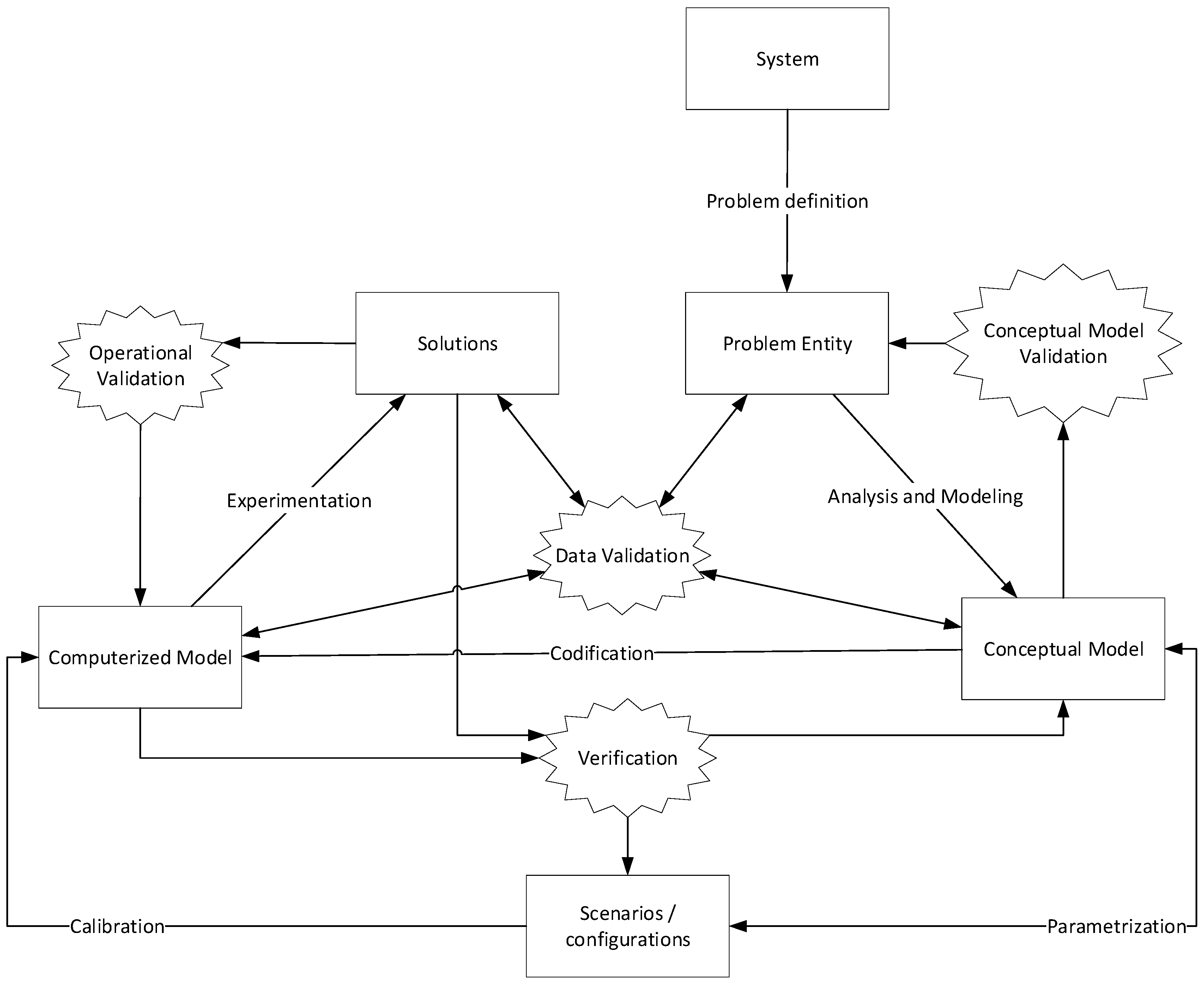
In this paper, we present this approach and we point to some preliminary results regarding the parametrization of our models. Figure 1 shows the process we follow to do the Validation of the models and the estimation of the model parameters.

In Figure 1, the products are represented by the squares, the validation actions on the stars, and the processes that transform a product to another product on the name of the arrow. We start analyzing the behavior of the pandemic and defining the problem we want to analyze, the Problem entity, that in our case is to model the propagation of the pandemic. With this, we define a Conceptual Model, and from it, we obtain a Computerized Model, a specific codification for our model. From this, we can obtain Solutions. However, the solutions must be validated, doing a Conceptual Model Validation, an Operational Validation a Verification, and a Data Validation.

Conceptual Model Validation in our approach is based on the refinements of the accepted System Dynamics SEIRD model (Susceptible, Exposed, Infective, Recovered and Deceased), and the agreement with the experts that these refinements make sense. The SEIRD acronym represents the sequence of the four basic containers in the SEIR model: Susceptible, Exposed, Infective, Removed. Additionally, the removed ones can be divided into two sub-containers, recovered and dead, as we do in our SEIRD approach. As we will see later, the discussion with the experts can increase the number of containers we will use in the model, to fit better with the experimental assumptions and with the data.

We do the conceptualization of the simulation model using Specification and Description Language (SDL). From this conceptualization, we obtain an automatic codification with SDLPS (https://sdlps.com). This new codification using SDLPS allows us to later extend the model to Multi-Agent simulation (MAS) or Cellular Automaton (CA) approaches, but we will not detail this in this paper. This allows us to work in a multi-paradigm simulation approach but keeping the parameters we estimate using the previous approaches and being able to use the previous models to validate our new assumptions. The Validation of a MAS or CA approaches is complex because the modeling process often follows the bottom-up approach, hence the comparison with other models and the use of these models as a reference, help us to define the constraints for these more detailed models.

Operational Validation will be based on the comparison between the three models we develop. We first define a conceptual model using System Dynamics, and we codify it using Insight Maker. We rewrite the model using Python, and then we execute the SDL model in SDLPS [2]; if the codification is correct, we expect to find the same results in the three models.

Data Validation will be focused on detecting if these model parameters are correct. In this specific model, the estimation of the parameters, as we will see later, cannot be obtained directly from the sources because of the novelty of the problem and the disparity of the methods used to obtain the data. This is the reason why here, Data Validation, along with the use of validated models (Operational and Conceptual Validations done) helps us to do an estimation of these parameters.

Notice that Verification is implicit on all these validation processes since we review the codification continuously, to assure that all is correct, however, we want to mention that since Insight Maker and SDLPS bases its execution on a correct conceptual model definition, the Verification process has been truly done only in the Python model we present.

In the next sections, we describe the three models we use to represent the same problem and how we use this approach for the Validation and the posterior Verification and Calibration of the model parameters.

2. System Dynamics Model

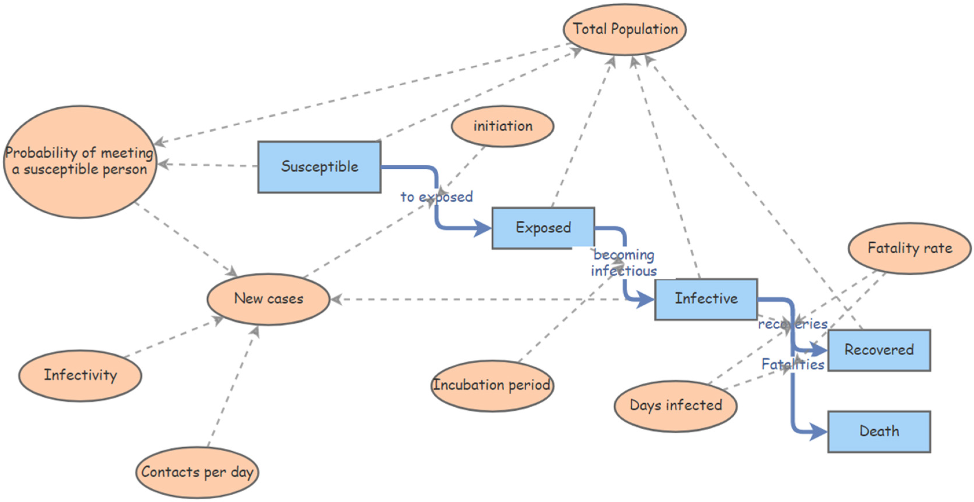
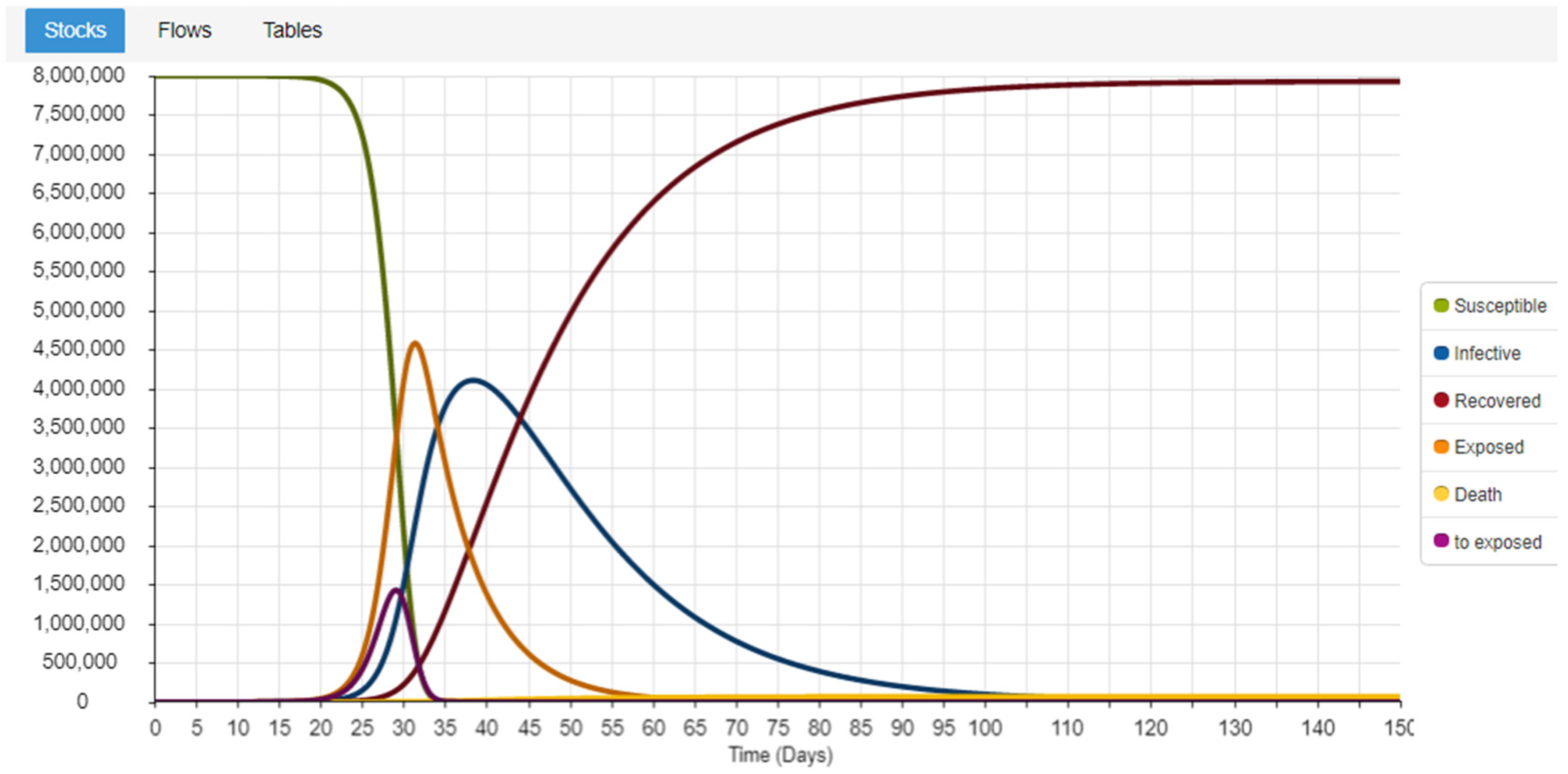
The first approximation to this problem is to model the behavior of the pandemic using a simple System Dynamic (SD) SEIRD approach [3,4], being focused on the Validations issues one can find in [5]. We start with a SEIRD model that can be found in [6], other similar models can be found in [7]. Figure 2 represents the Forrester diagram of the model, while Figure 3 presents the simulation results using the parametrization we use, to do the comparison with other models’ validation techniques.

The parametrization we use in this model is used to test the different models in the model comparison approach. We will not obtain conclusions regarding the system yet; this is only used to assure that the definition of the different models we own, and specifically the SDL conceptual model we want to extend later, are correctly defined.

3. SDL Conceptual Model

Specification and Description Language (SDL) is an object-oriented, formal language that was defined by the International Telecommunication Union–Telecommunication Standardization Sector (ITU–T), The document that defines the language structure is the Recommendation Z.100 [8].

Originally, the language was designed to specify event-driven, real-time, complex interactive applications that involve many concurrent activities. The mechanisms used to perform the communication between the different model elements are discrete signals [9,10]. In addition, the use of SDL to perform the conceptualization of the simulation model allows the extension of the model to be able to integrate CA [11,12] or MAS [13] simulation paradigms, combining them in a single model, or connecting the model with other simulation models or simulators. It also has strong capabilities to integrate IoT [14], which will be interesting in future developments of this research to interact with different sensors. Moreover, the language can be transformed into other well-known formal languages, like DEVS [15], allowing the common formalism approach [16] for complex simulation.

The conceptualization of a simulation model needs to define the next components: (i) Structure: system, blocks, processes, and the hierarchy of processes. (ii) Communication: signals, including the parameters and channels that the signals use to travel. (iii) Behavior: defined through the processes. (iv) Data: based on Abstract Data Types (ADT). (v) Inheritances: describe the relationships between and the specializations of the model elements. At least the first two-components, the structure, and the behavior must be described in a formal language to be able to do a correct conceptualization of a simulation model.

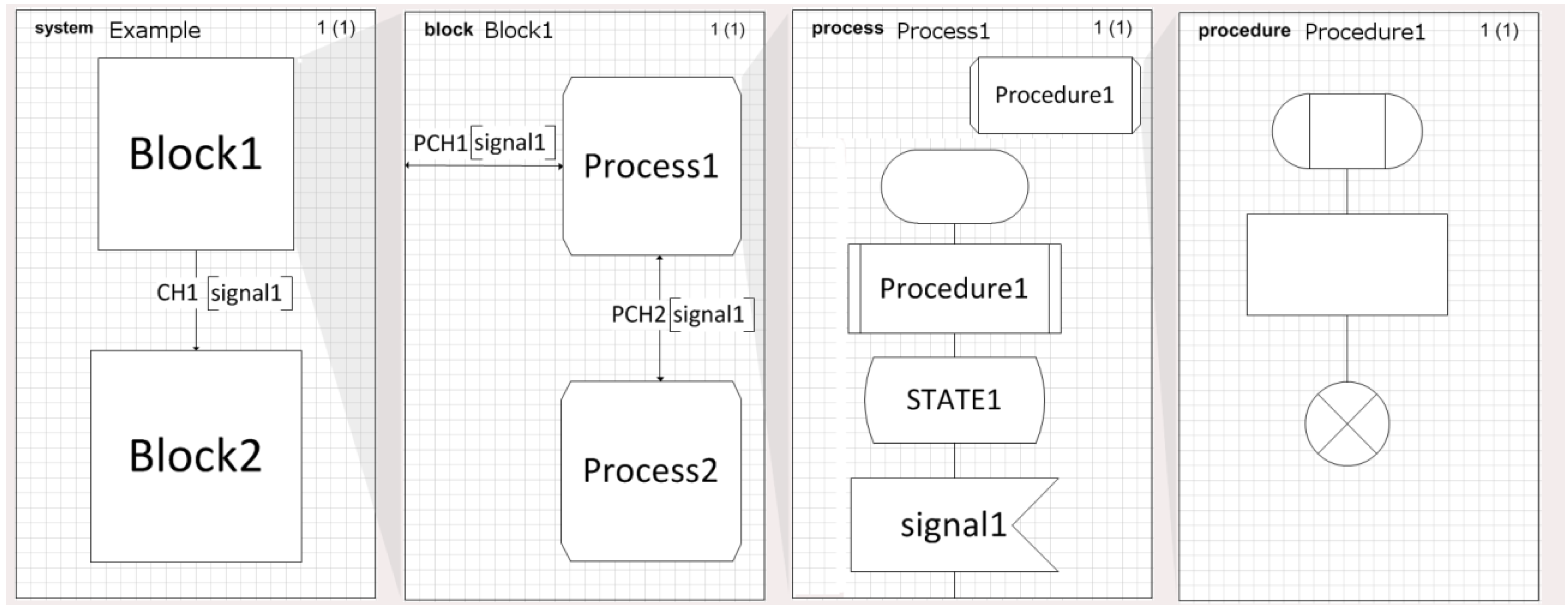
The language has four levels: (i) system, (ii) blocks, (iii) processes, and (iv) procedures. The hierarchical decomposition of SDL is shown in Figure 4. Regarding the notation we will use to describe the SDL diagrams, every time we refer to an SDL element, we write it all in CAPS, while the name of the elements will be in Italics.

A SYSTEM diagram represents the uppermost level of the structure of the model, and the communications between them, the channels. Since the SYSTEM is the outermost agent, it may communicate with the environment. The SYSTEM, in SDL terminology, is an AGENT but is not the only AGENT we can find, the BLOCK and the PROCESS that we will find in the lower levels are also AGENTS.

Both bidirectional and unidirectional channels are allowed in SDL. The communication channels are joined to the objects through ports. Ports are important elements because they guarantee the independence of the different AGENTS we will use in our models. This is important to allow simulation objects, AGENTS, reuse. An object only knows its ports, which are the doors through which it communicates with its environment. An AGENT only knows that it sends and receives events using a specific port.

SYSTEM diagrams and BLOCK diagrams represent the model structure, the hierarchical decompositions of the different model elements; some good examples can be reviewed in [10]. However, a PROCESS diagram defines the behavior of the model. When an AGENT PROCESS receives a specific SIGNAL, as a trigger, a set of actions are executed in no time. The time is related to the SIGNAL as a delay needed to travel to another AGENT. A PROCESS diagram uses different graphical elements to represent its behavior. In the next lines, we describe synthetically some of the more important elements to simplify the understanding of the posterior pandemic model definition.

Start. This element defines the initial condition for a PROCESS diagram.

State. The state element only contains the name of a state, defining the states of behavioral diagrams, such as PROCESS diagrams.

Input. Input elements describe the type of events that can be received by the process. All branches of a specific state start with an Input element because an object changes its state only when a new event is received.

Create. This element allows the creation of an agent.

Task. This element allows the interpretation of informal texts or programming code. In this paper, following SDL-RT (1), we use C code.

Procedure call. These elements perform a procedure call. A PROCEDURE can be defined in the last level of the SDL language. It can be used to encapsulate pieces of the model for reuse.

Output. Output elements describe the types of signals to be sent, the parameters that the signal carries, and the destination. If ambiguity about the signal destination exists, communication can be directed specifying destinations using a processing identity value (PId), an agent name, or using the sentence via path. If there is more than one path and no specific output is defined, an arbitrary one is used. The destination value can be stored in a variable for later use. Four PId expressions can be used, (i) self, an agent’s own identity; (ii) parent, the agent that created the agent (Null for initial agents); (iii) offspring, the most recent agent created by the agent; (iv) sender, the agent that sent the last signal input (null before any signal received).

Decision. These elements describe bifurcations. Their behavior depends on how the related question is answered.

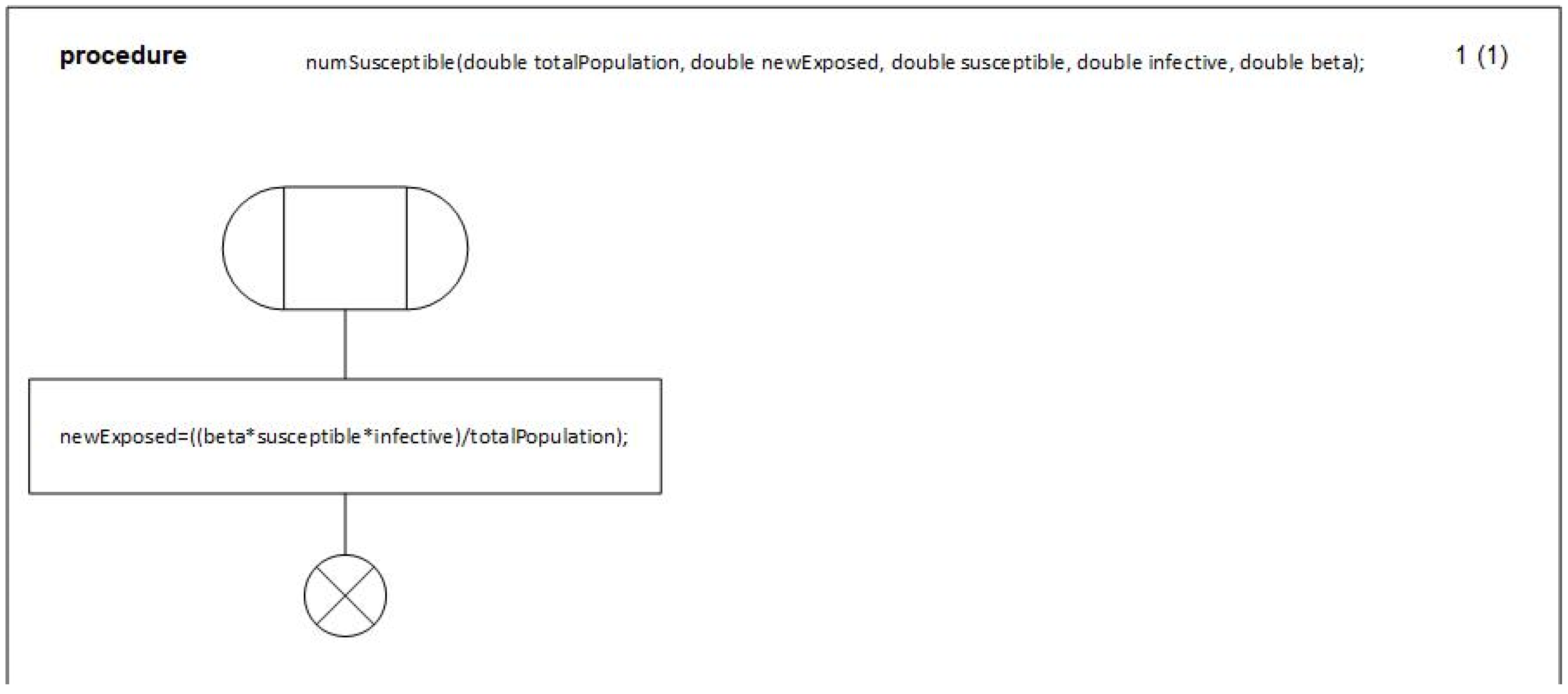
The last level of the SDL language (PROCEDURE diagrams) allows the description of procedures that can be used in the PROCESS diagrams through the procedure calls . These diagrams are remarkably like the PROCESS diagrams with the exception that they do not need to state definitions, a PROCEDURE is just a piece of code, but not an AGENT.

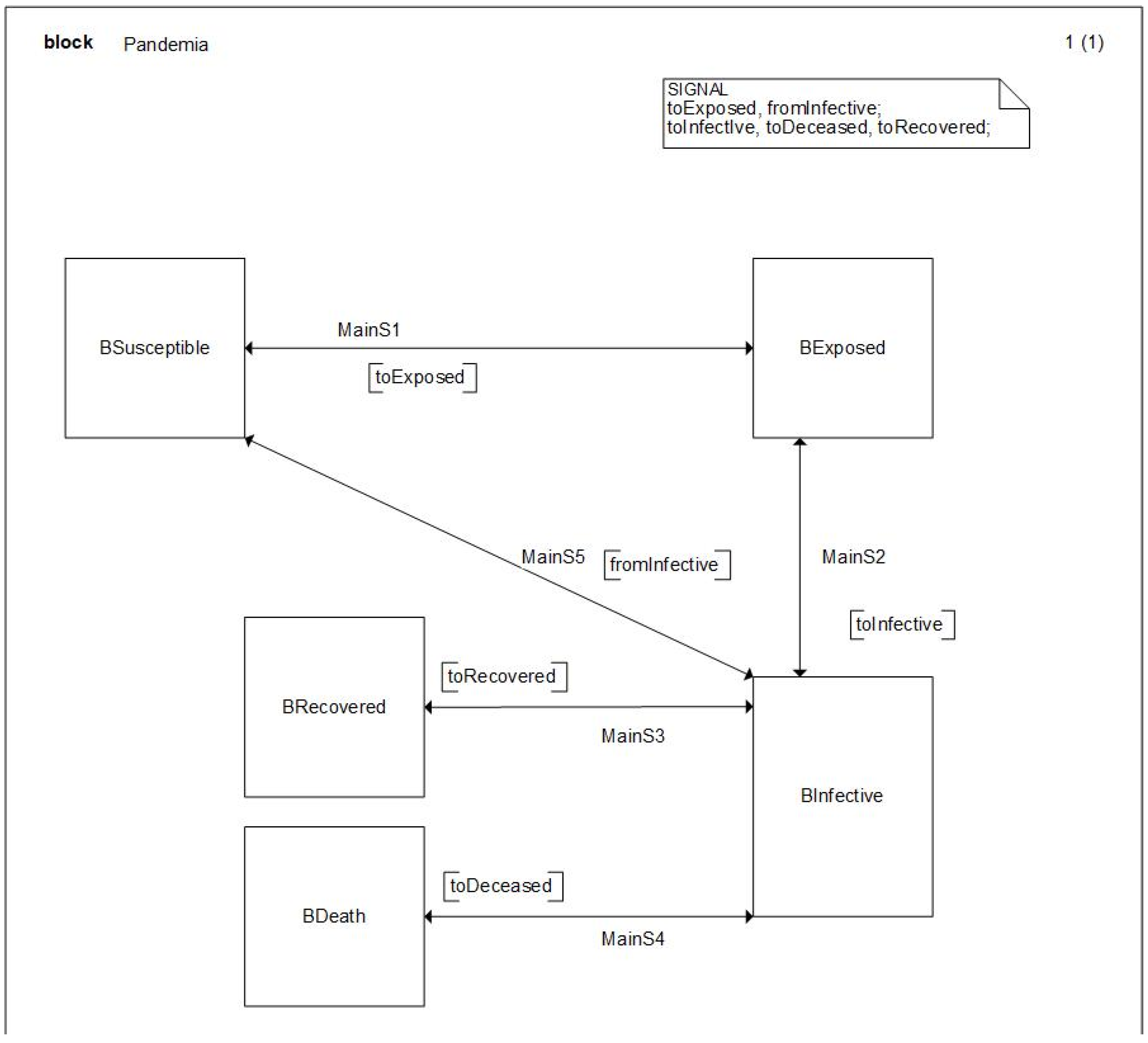
With all this initial consideration, we describe next the model that explains the expansion of the pandemic formalized in SDL. First, we will start with the SYSTEM diagram, presented in Figure 5, which represents the initial point to understand the model structure and the model’s main AGENTS.

As one can notice, this diagram shows the main LEVELS of the system dynamic model previously presented as SDL BLOCKs, allowing a graphical definition of the model that is remarkably like the System Dynamics definition. The continuous nature of SD models is not a problem for SDL that owns a continuous capability. However, in that case, we opt for a discretization of the time, which is a similar approach to that followed by Insight Maker, and we will be able to select the ${∆}_t$ to be used as the model time steep, following the Activity scanning approach. The details of the model are presented in the next figures, also you can refer to the website of the tool at https://sdlps.com.

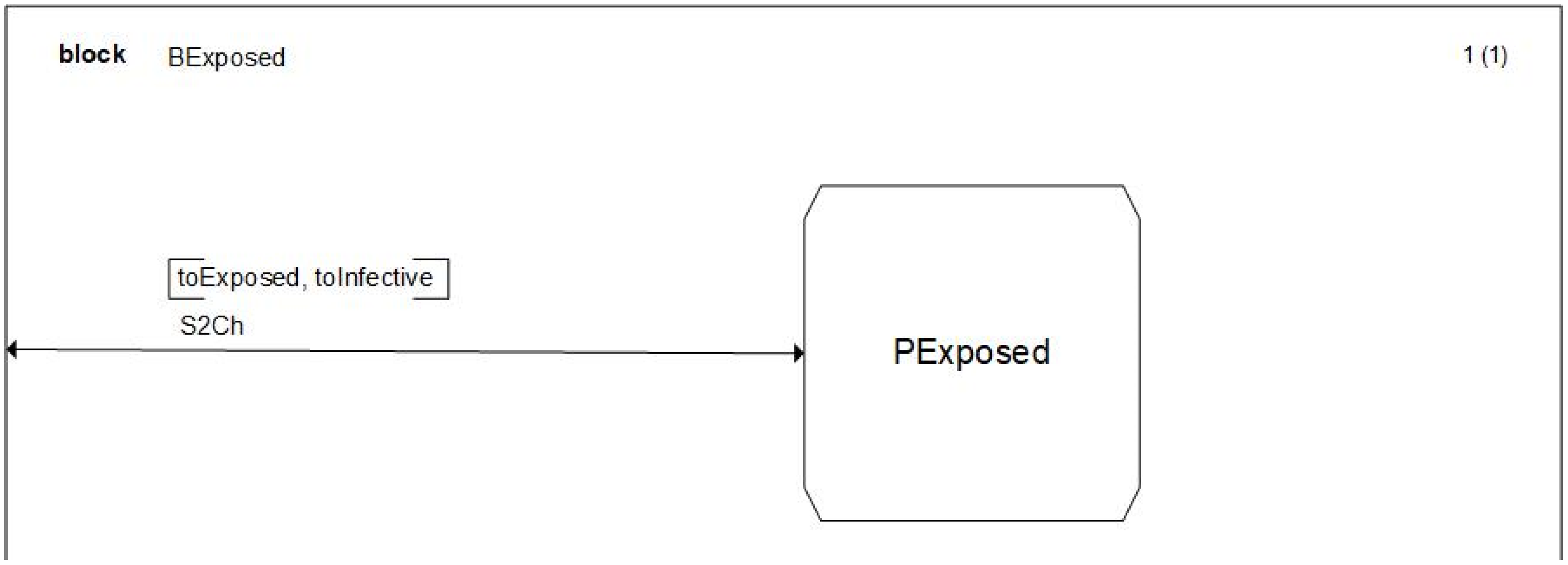
The definition of a model in SDL is modular; this implies that, at every level, we detail the characteristics of the model a little more. As an example, if we enter on the details of the BSusceptible BLOCK we will see the PROCESS that drives the structure of this BLOCK. Since this is not of interest in this paper, we will only show one of these diagrams, see Figure 6, and we will go further to the PROCESS diagrams that detail the model behavior. However, the complete characterization of this model can be downloaded on the website provided in the supplementary material section.

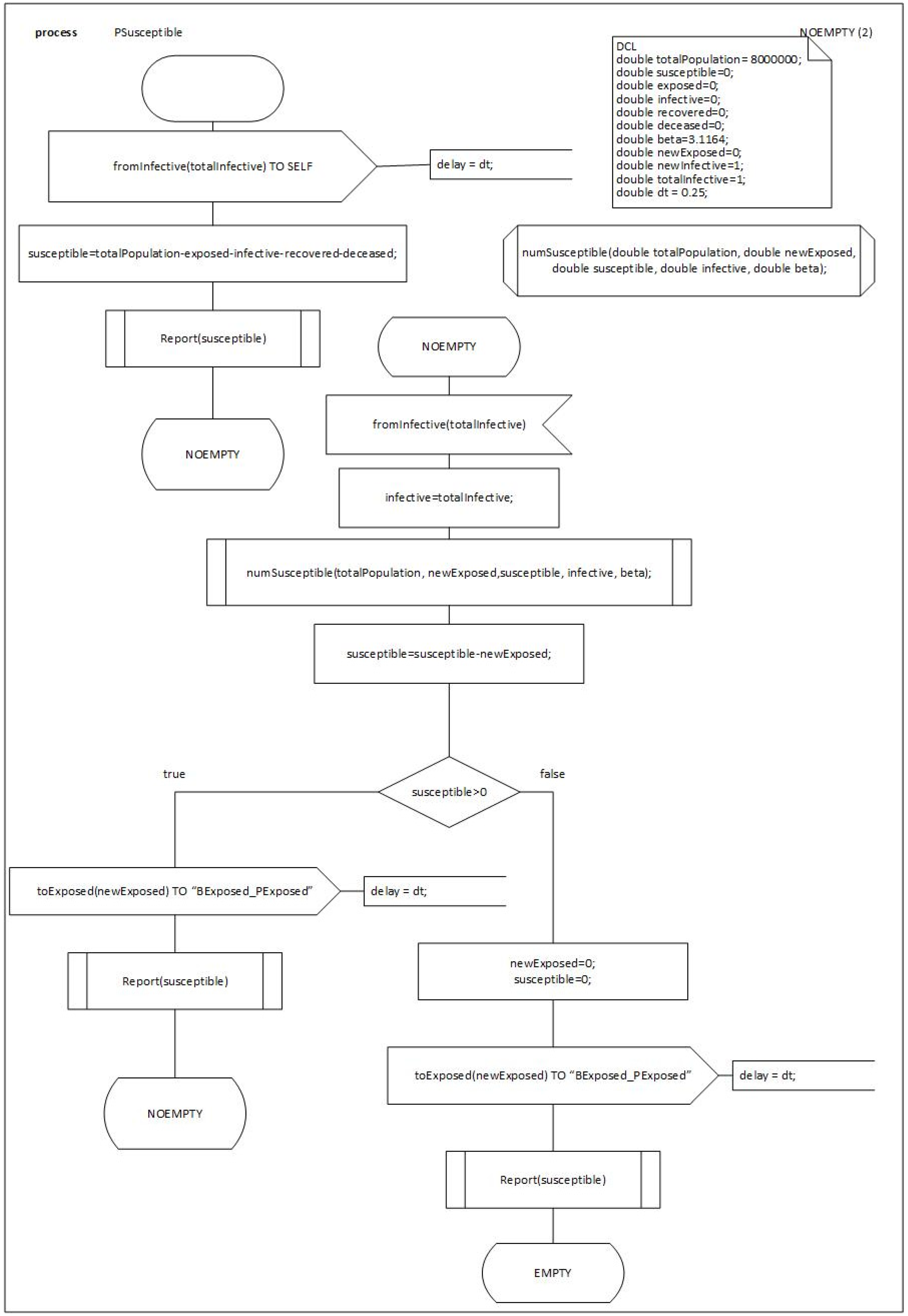
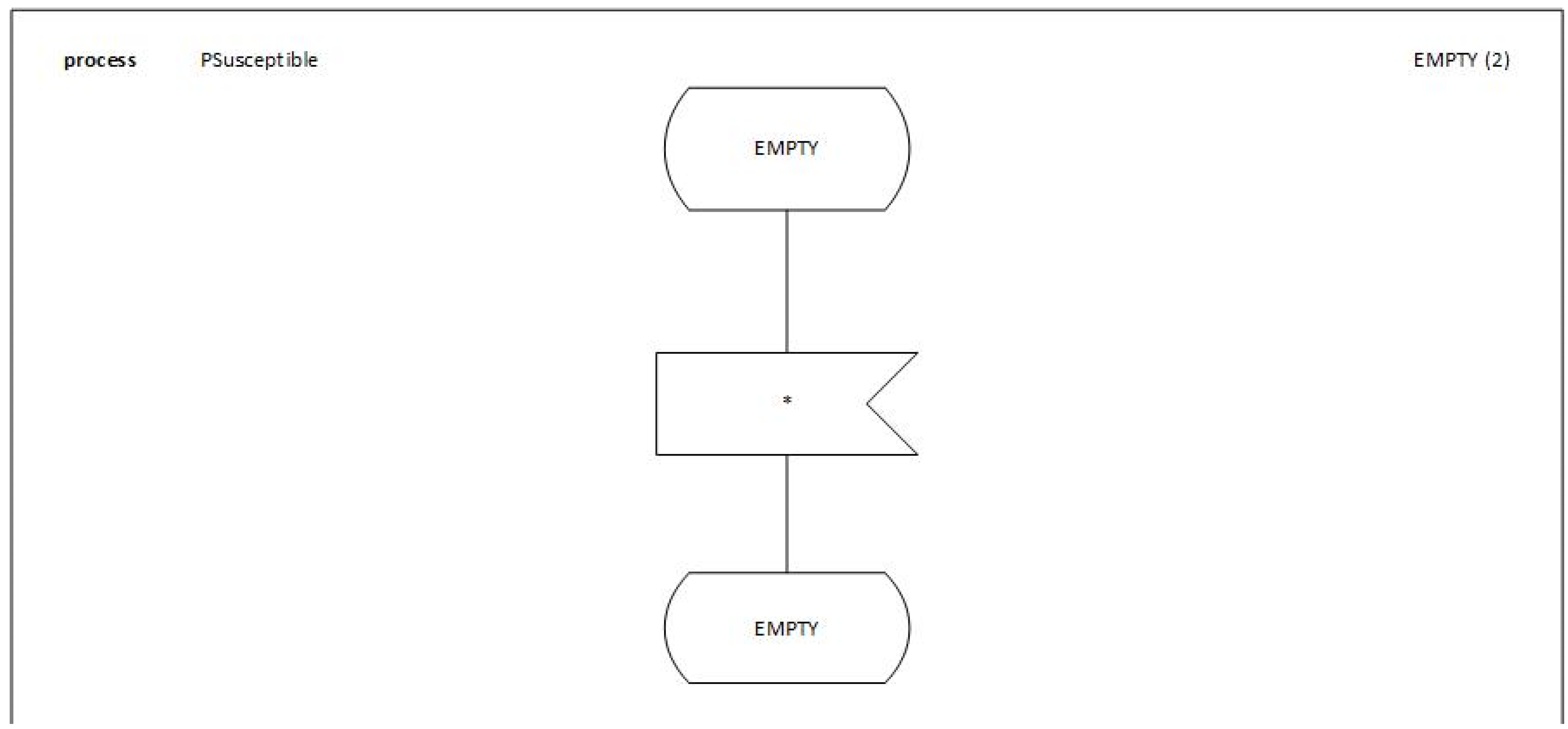
We will detail the behavior and the process of the first BLOCKs of the model PSusceptible, see Figure 7, Figure 8 and Figure 9.

Notice that this model is a discrete model that can be expanded to a Cellular Automaton model [11] or a Multi-Agent Simulation model [13]. This conceptualization allows us to explain the details of the different compartments in the SEIRD model to non-specialists and discuss graphically the model assumptions.

4. Python Codification and Parameter Fitting

From these models, we obtain a third codification using Python. This is the codification we will use for the calibration and parameter fitting, and we will compare the results and the assumptions used with the previous two models. To do so, we will be focused on four variables for the model calibration using the observed data. Two refer to data quality and two to confinement quality:

1.

The time lag in the publication of the data.

2.

The degree of underreporting in the numbers of newly infected.

3.

The timing of the adoption of containment and confinement policies.

4.

The containment factor (ρ) that quantifies the power of these measures.

A fifth parameter is the transmission rate of the disease represented, as we will see later, by the beta coefficient in the system dynamics equations, see Equations (1)–(6).

$$S^{\prime }\left(t\right)=-\frac{\beta S\left(t\right)I\left(t\right)}{N}$$

(1)

$$E’\left(t\right)=\frac{\beta S\left(t\right)I\left(t\right)}{N}-\alpha E$$

(2)

$$I’\left(t\right)=\alpha E\left(t\right)-\gamma I\left(t\right)$$

(3)

$$R’\left(t\right)=\gamma \left(1-\mu \right)I\left(t\right)$$

(4)

$$D’\left(t\right)=\gamma \mu I\left(t\right)$$

(5)

$$N=S+E+I+R+D$$

(6)

The alpha (latency rate) and gamma (recovery rate) parameters will be considered constant, based on the measurements made by other studies and N will be the total population, assuming that there is no pre-existing level of immunization to SARS-Cov2 and that therefore the whole population is initially susceptible ($S_0=N$).

The mean incubation period (1/α) and the mean infectious period (1/γ) can be obtained by the inverse of the above parameters. The fatality rate (µ) gives us the fraction of sick people who do not recover. Regarding the transmission rate, this could be represented as the product of the contact rate per day and infectivity to make more detailed modeling.

Finally, we will use a simulated annealing algorithm called “dual annealing” included in the SciPy libraries to proceed with the multiparametric optimization by least-squares minimization. In addition, we will also be able to estimate a value for the effective (Reff) and the basic reproduction number (R0) from the containment factor (ρ), the transmission rate (β) and the recovery rate (γ) with the Equation (7). The basic reproduction number, R0, see [17], represents the average number of secondary cases that result from the introduction of a single infectious case in a totally susceptible population during the infectiousness period. In turn, the effective reproduction number, Reff, is the same concept but after applying the containment measures.

$$R_{eff}=\rho R_0=\frac{\rho \beta }{\gamma }$$

(7)

5. Comparison with Other Models’ Validation

From these different codifications, and since we want to assure that they are correct, first, we start with a comparison with other models’ validation process. This helps us to assure that the codifications we do following the different approaches are correct, hence, the conclusions we obtain can be considered as valid.

To do so, we perform a calibration between the different codifications. We analyze the results we obtain from the different models and determine if the different codifications have been done correctly and if they correctly represent the assumptions.

The preliminary parameters that allow us to conduct the validation between the different codifications are presented in

Table 1. Parameters for the validation between the different models.

Parameter	Value
beta	contactsday × infectivity
alpha	1/incubationPeriod
gamma	1/infectiousPeriod
contactsday	7.42
infectivity	0.42
infectiousPeriod	14.39
incubationPeriod	6.38
fatalityRate	0.85

.

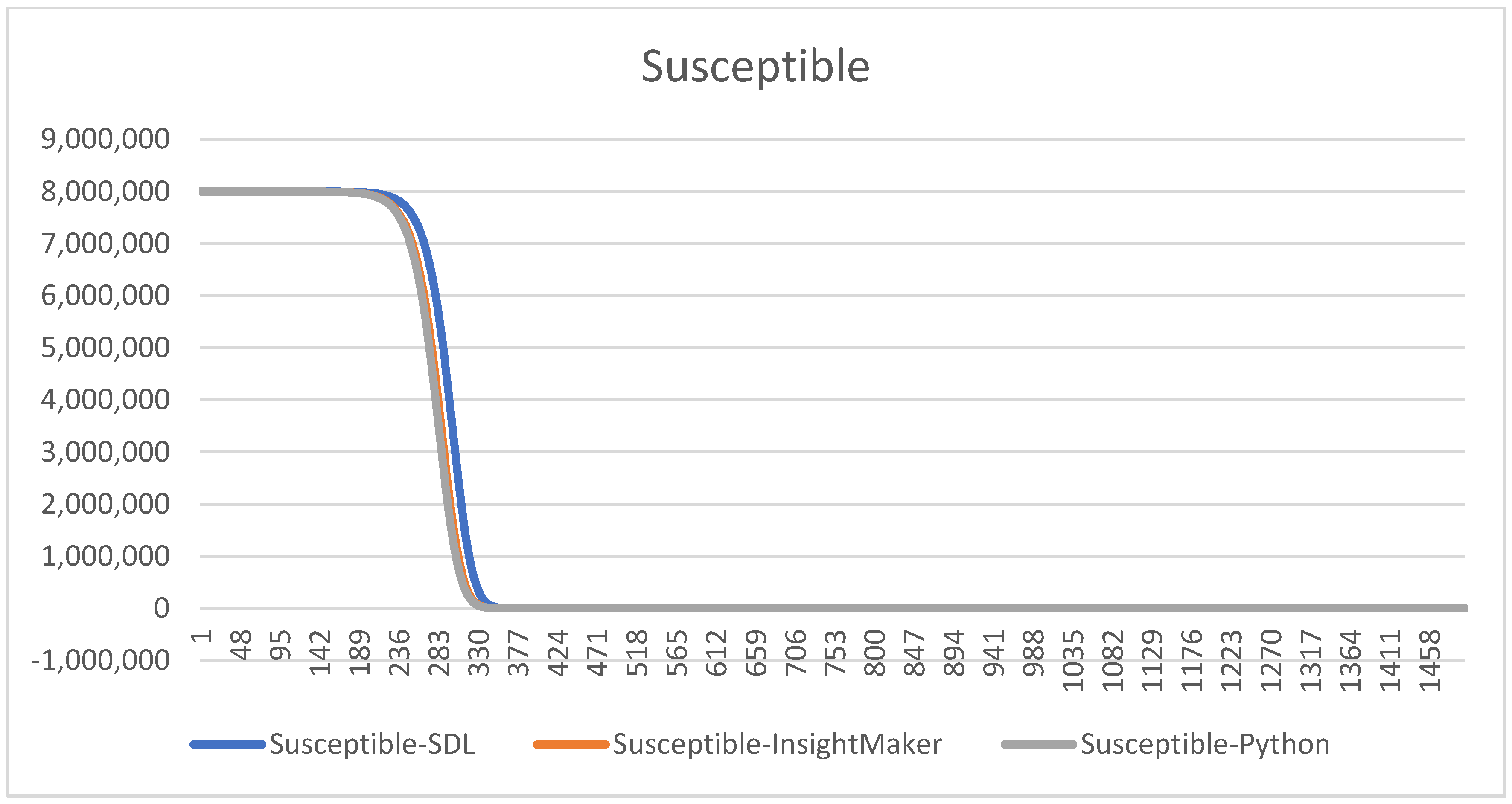
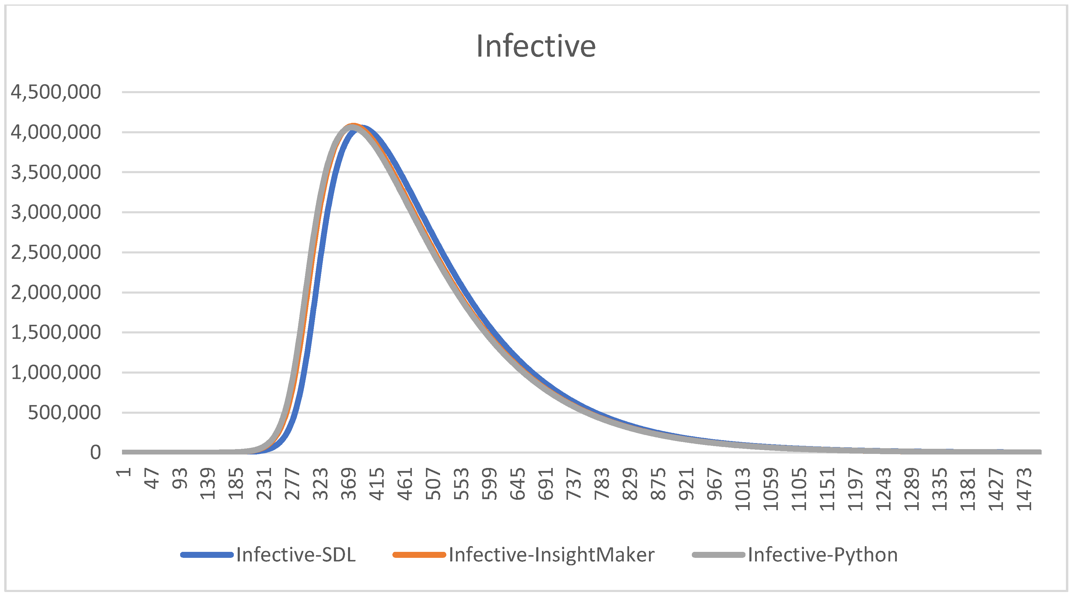
With these parameters, we compare the three different models graphically to understand if the results are similar, hence whether the models can be considered as valid, see Figure 10 and Figure 11.

Notice that using the same ${∆}_t=0.1$, the charts are all the same. We remark that this validation process consumes time, but thanks to it we will able to detect some errors on the codification in Python and in the SDL conceptualization and Insight Maker codification. Some of them are subtle, since the models provide curves that seem correct but that have some errors. This comparison helps to increase our confidence, and the confidence of the experts and decision-makers, on the models.

6. Parameters Validation

Once the models seem to behave correctly, we can go further and find the parameters that better define the behavior of the system, in our case using the Python codification, with the main cases where we have data. Other approaches like [18] have been done to infer the parameters of the novel COVID-19 infection. We are focused on South Korea and Spain. This will help us to estimate the final parameters to conduct the experiments and to understand that the results we are obtaining from the models are accurate enough to predict the behavior of the whole system’s evolution. All observational data used to fit the models have been obtained from the Worldometer database [19] and the Johns Hopkins University CSSE repository [20].

Firstly, we assume for all simulations the value of 5 days for both the mean incubation period (1/α) and the mean infectious period (1/γ) based on the studies [21,22], respectively.

Secondly, we assume the existence of at least one turning point that determines the timing of government intervention to contain the spread of the disease. Each changing point will require the adjustment of two parameters, the containment factor, and the starting point. Knowing the exact date of the intervention also enables us to infer the delay in reporting cases.

6.1. South Korea Case

Due to its strong and early response to the virus, we consider the time series from South Korea as a good reference. As an ideal assumption, the Korean data are not underreported in our preliminary analysis. The level of reporting is, however, unknown and, according to [23], it would be in the range of 50 to 100% of the total real cases.

It is important to note that not all cases reported as positive develop the disease. Recent studies in Korea [24] and China [25] have set the case fatality rate (CFR, the fatality rate of detected cases) at 1.4%, substantially lower than initial reports. However, the infection fatality rate (IFR, the fatality rate of total infected population) remains highly uncertain due to the lack of reliable estimates on the number of asymptomatic cases. In our study, we have established a possible upper bound. So, if Korea’s underreporting were higher, the IFR would decrease accordingly.

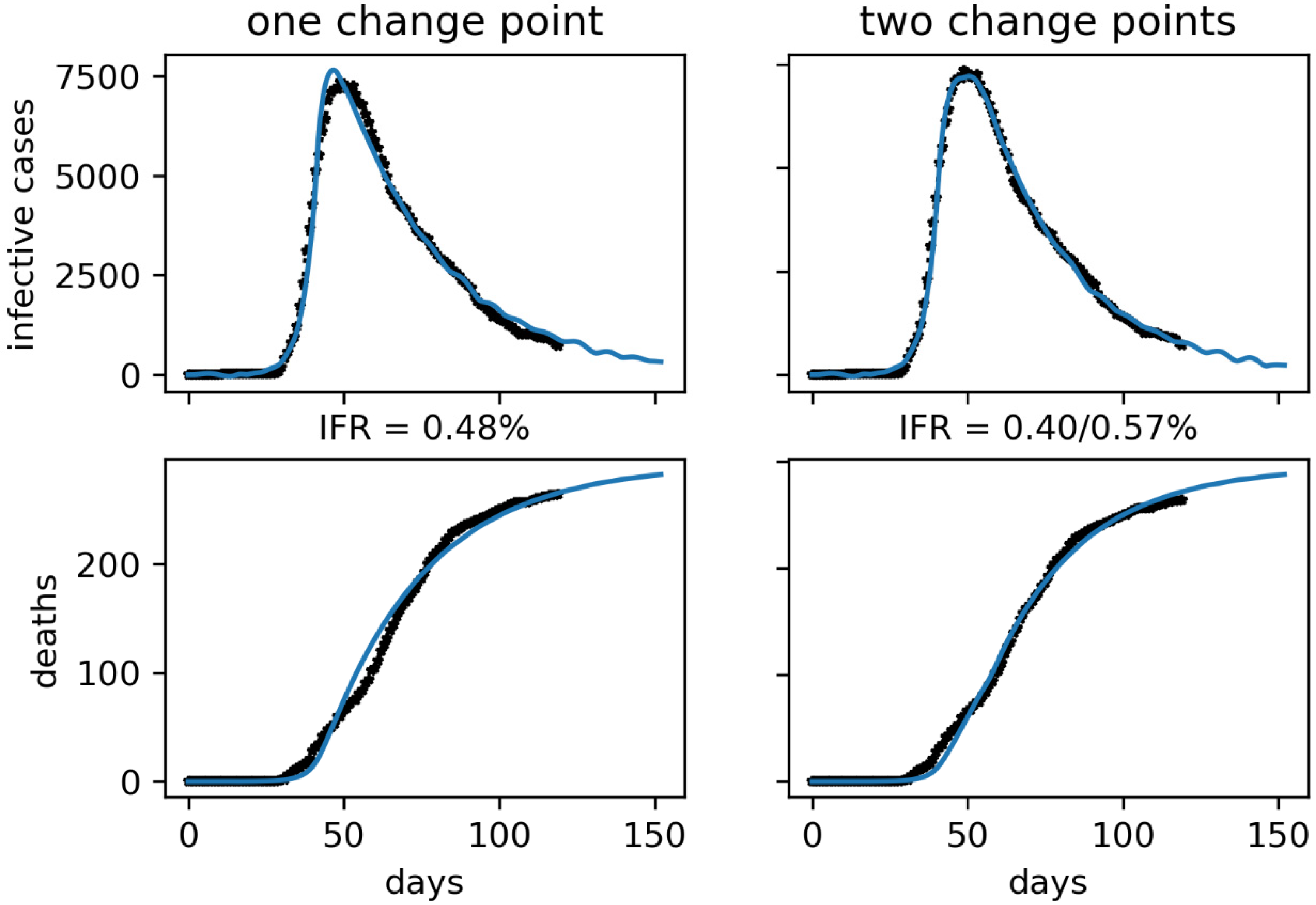
We have first reproduced the curve of confirmed active infectious cases knowing that the first lockdowns and serious containment measures taken by the government happened between February 20 and 25. However, these effects will be noticed days later due to the delay in diagnosis and publication of the data. For Korea, we have estimated a delay of around 10 days on average from the infectious contact to the confirmation of the case, which includes the 5 days of latency and the 5-day infective period see Figure 12 and Figure 13.

The results of our approach are consistent with other techniques such as the time series correlation analysis [26] where a range of 0.4 to 0.7% is calculated for the Korean IFR, an interval that includes all our proposed values. But these are only higher estimates assuming no underreporting. The actual value should be even lower as more comprehensive studies seem to indicate. They estimate it at 0.1 to 0.4 according to the CEBM [27] or even slightly less than 0.1 according to [28].

All this leads, in turn, to a higher R₀ value than initially estimated (2.2–2.7). The Imperial College raised it in its March 30 report [29] to 3.87 [3.01–4.66] and the CDC published, on April 7 [30], an even more dramatic update raising R₀ to 5.7 [3.8–8.9]. The latter values are in line with those obtained in our fits. Of course, there is still a lot of uncertainty around these values but a relatively high value of R₀ is already a reasonable hypothesis.

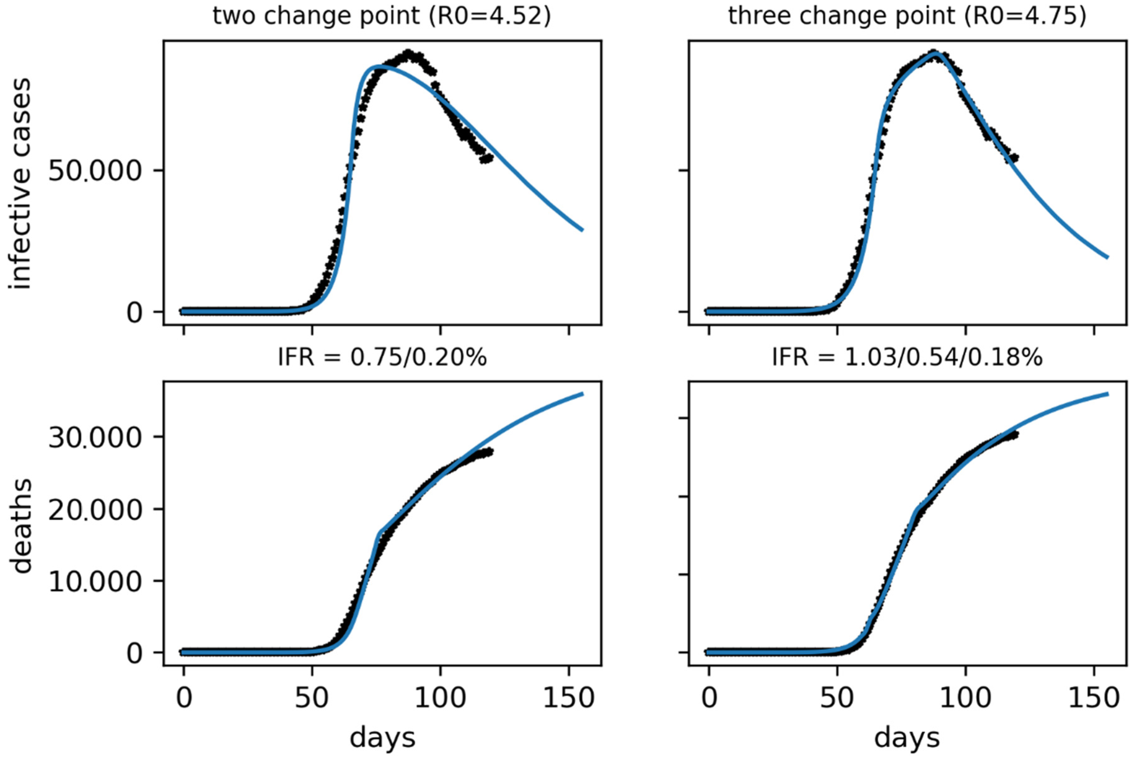
6.2. Spain Case

In this case, we have assumed a very low infectious reporting of 10%, under the results of [23]. We also expect that the data on confirmed cases will be of much lower quality than in Korea, possibly not only because of a high underreporting but also because of a longer delay in data collection and an unknown time dependency in both respects. Higher mortality is also expected than in Korea due to an older population, a more overwhelmed health system and delayed detection of cases. Its value will also most likely be variable over time, increasing first due to the health system saturation and decreasing at the end, due to its decongestion. In Spain, the application of containment measures began late, on 10 March, and was tightened up in the following days, on the 14th with the start of the confinement and the 28th with the almost total closure of the country. Given the progressiveness of its implementation, we will see that the model will better adjust to multi-step containment factors. The severity of these lockdowns is demonstrated by the reduction in mobility reported by Google [31].

It is important to note that the parameters obtained for Spain are probably only one of several possible configurations. Further studies will be necessary to clarify which of these would be the correct one. For example, varying the mortality or reporting of both infectious and deaths can have the same effect and all of them can change over time. As in the study done with Korea, it will be necessary to simultaneously fit the infectious and death curves.

7. Discussion

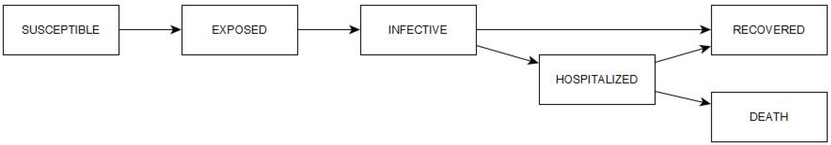
With the SEIRD approach, we have not been able to fit the active and cumulative case curves simultaneously. To achieve this, it will be necessary to extend the model to a SEIHRD type by adding the hospitalized compartment as shown in Figure 14. This is due to the high heterogeneity in the prognosis of the disease, in which approximately 80% of those affected have mild or moderate symptoms and the remaining 20% are severe, sometimes fatal [32]. This disparity in prognosis means that the recovery time for the latter is much longer than for the former. In the basic SEIR model, recovery time is equal to the infectious period, but this is not the case for hospitalized patients. Moreover, it is precisely expected that in confirmed cases they should present a strong bias in favor of severe cases, making the basic SEIR model insufficient.

All of the process presented allows us to define credible models that can be expanded and validated. With this premise, we can add containment measures that affect two parameters, the Susceptible population, and the rate of infection. The initial parametrization is based on the suggested current data. The containment measures, if this model is true, must be reinforced to contain the propagation of the pandemic due to the high possibility of asymptomatic cases; once the curve flattens, extensive testing will be needed to ensure that, after 15 days, no one is still infected.

With all this process we will able to find an initial set of parameters for our models, which are summarized in

Table 2. Model 1 corresponds to a one change point scenario, and model 2 to a two change points scenario. To each change point corresponds a contention factor and a contention date, representing the intensity and the timing of each change, (*) days after 22 January 2020.

Parameter	Notation	Model 1	Model 2	Remark
Initial susceptible population	S0	51.6 million	51.6 million	S. Korea population
Transmission rate	β	0.952	0.957	Fitted parameter
Contention factor	ρ	0.1372	[0.1834, 0.1295]	Fitted stepwise function
Contention start dates *	t (ρ)	41.56 days	[40.19, 52.26]	Fitted intervals
Mean incubation period	α−1	5 days	5 days	(Lin et al. 2020)
Mean infectious period	γ−1	5.4 days	5.4 days	Fitted in model 1
Infectious fatality rate	µ	0.48%	[0.40, 0.57]	Fitted stepwise function
Basic reproduction number	R0 = β/γ	5.16	5.19	Calculated

for the Korea case. Notice that this is an initial result that must be contrasted continuously with new datasets and with the new models that increase the capabilities to represent the reality.

While the purpose of this article is not to delve into the parameterization of the epidemic, it is clear that a more exhaustive analysis, considering more countries and with a deeper and more robust exploration of the parameter space, could allow us to better infer the values of the model from comparative studies. One thing is clear; the hypothesis of higher R₀ in the range 5 to 6 and lower IFR of 0.3 to 0.7 seems increasingly feasible. If this were the case, the deconfinement strategy should take this into account. We notice also that the parameters of the model will be affected by the containment measures, hence they will change during the pandemic process. The hidden reasons for this can be analyzed with more detailed models, where MAS techniques can become a key ingredient to glimpse the causality that rules the behavior of citizens in a confinement process.

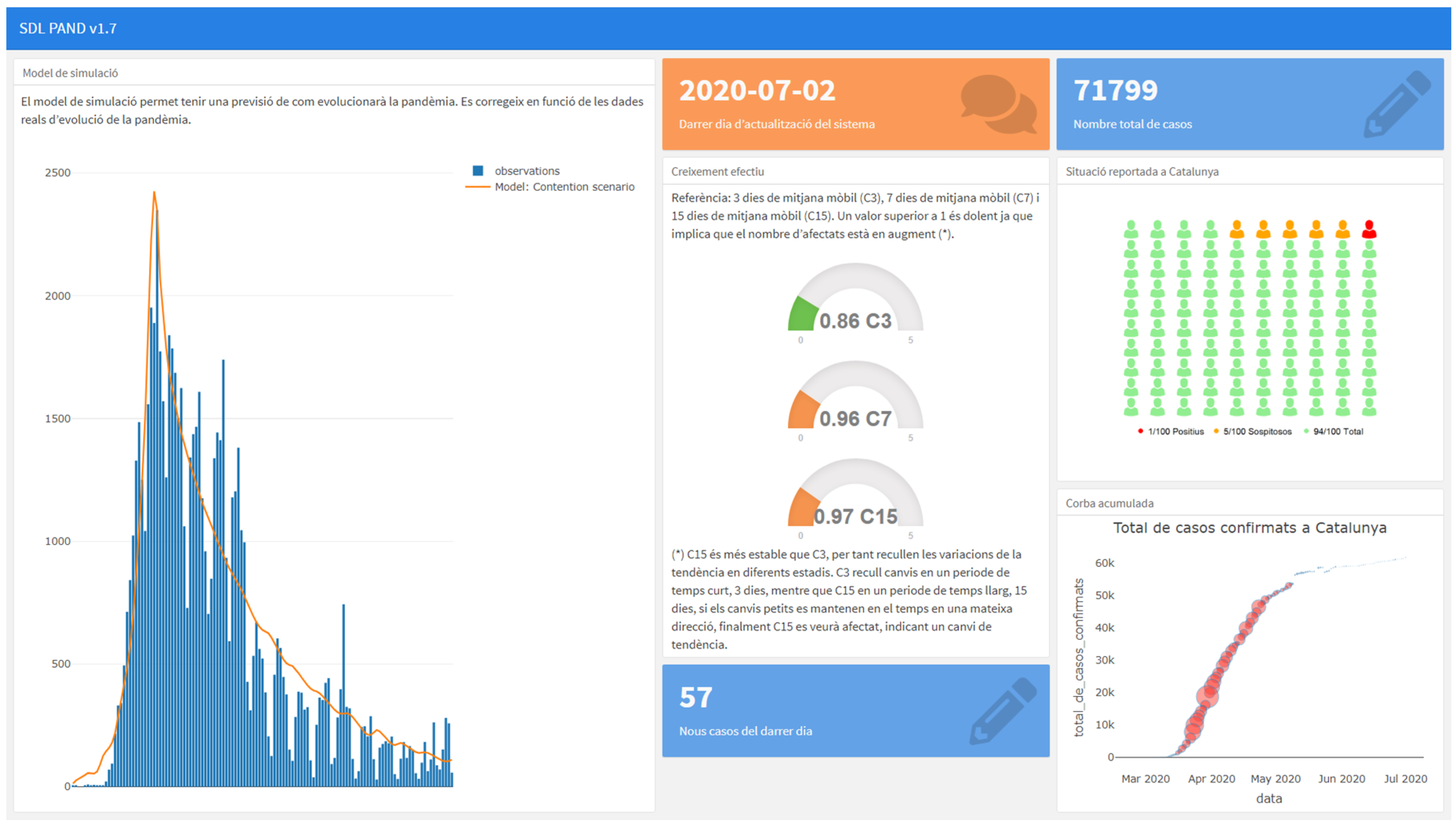
This model is now integrated into the first version of a Decision Support System that generates information regarding the evolution and the current state of the pandemic situation in Catalonia, see Figure 15. The application can be accessed at https://sdlps.com/projects/documentation/3.

In this system, we use a continuous validation process comparing the different models and analyzing the model hypotheses represented in the SDL diagrams. In the system, a statistical test is executed every time the data obtained from the system is updated (for example, the number of new cases, daily). This serves as an automatic warning to detect if the model is no longer valid, hence its hypotheses and parameters need to be reevaluated to obtain a good prevision. In that case, we review the conceptual model (SDL model) with the specialists, and we upload a new model with the new proposed model or parametrization.

8. Conclusions

Here, we have a SEIRD model and we will investigate what changes would be appropriate in the parameters for modeling the 2019 Coronavirus. Due to the complexity in understanding if the data we are using is correct, simulation represents an excellent approach to cope with the uncertainty in depicting the causality.

The questions that we want to answer in this kind of model are not the shape of the curves, that are almost known from the beginning, but when something happens, hence, the amplitude and the height of the shapes. This is crucial, since in the current circumstance, it implies the collapse of certain resources, not only healthcare. The validation process hence becomes critical and allows us to estimate the different parameters of the model from the data we obtain, more so if we pretend to extend the well-known models to more complex approaches.

The simulation approach makes it possible to detail explicitly something that is crucial to make decisions; the causality. We can infer this from the assumptions that are represented in the conceptual model, and from it, we can make decisions to improve the system behavior.

The conceptualization of the model using SDL diagrams is one of the approaches one can use to draw graphically the model assumptions. This allows the opening of the model’s understanding to a wider number of specialists, to simplify the maintenance and improve collaborations. Moreover, SDL specifically makes it possible to expand and combine the model with other paradigms like MAS [33] or CA [11] in a hybrid simulation scenario, or combine the simulation model with real-time data, obtained from open data sources or IoT devices [14], to simplify the solution validation of the model, see an example of this approach here [34].

In the paper we also present a parametrization of the models by doing a comparison with two different datasets. This seems to work correctly; however, this must be analyzed continuously during the evolution of the pandemic process.