Multiresolution Speech Enhancement Based on Proposed Circular Nested Microphone Array in Combination with Sub-Band Affine Projection Algorithm

Abstract

Speech enhancement is one of the most important fields in audio and speech signal processing. The speech enhancement methods are divided into the single and multi-channel algorithms. The multi-channel methods increase the speech enhancement performance by providing more information with the use of more microphones. In addition, spatial aliasing is one of the destructive factors in speech enhancement strategies. In this article, we first propose a uniform circular nested microphone array (CNMA) for data recording. The microphone array increases the accuracy of the speech processing methods by increasing the information. Moreover, the proposed nested structure eliminates the spatial aliasing between microphone signals. The circular shape in the proposed nested microphone array implements the speech enhancement algorithm with the same probability for the speakers in all directions. In addition, the speech signal information is different in frequency bands, where the sub-band processing is proposed by the use of the analysis filter bank. The frequency resolution is increased in low frequency components by implementing the proposed filter bank. Then, the affine projection algorithm (APA) is implemented as an adaptive filter on sub-bands that were obtained by the proposed nested microphone array and analysis filter bank. This algorithm adaptively enhances the noisy speech signal. Next, the synthesis filters are implemented for reconstructing the enhanced speech signal. The proposed circular nested microphone array in combination with the sub-band affine projection algorithm (CNMA-SBAPA) is compared with the least mean square (LMS), recursive least square (RLS), traditional APA, distributed multichannel Wiener filter (DB-MWF), and multichannel nonnegative matrix factorization-minimum variance distortionless response (MNMF-MVDR) in terms of the segmental signal-to-noise ratio (SegSNR), perceptual evaluation of speech quality (PESQ), mean opinion score (MOS), short-time objective intelligibility (STOI), and speed of convergence on real and simulated data for white and colored noises. In all scenarios, the proposed method has high accuracy at different levels and noise types by the lower distortion in comparison with other works and, furthermore, the speed of convergence is higher than the compared researches.

1. Introduction

In the current century, the smartphones and other communication devices have been an important part of human life, where it is impossible to have social communications without them [1,2]. One of the principal parts in these smartphones is the signal processing platform. This part has an important role in the telecommunication and audio signal processing. Denoising and dereverberation are two main sections in the signal processing and enhancement platforms, which is the aim of this article, to increase the performance of speech enhancement algorithms [3]. Increasing the number of sensors improves the accuracy of denoising algorithms due to the spatial spectrum extension by providing the proper information. The definition of accuracy in the enhancement algorithms is how the enhanced signal is closer to the original signal with a high level of noise elimination and less distortion. Therefore, the speech enhancement is the main part in such applications as: hearing aid systems, mobile communication, speaker localization and tracking, speech recognition, voice activity detection (VAD), speaker identification, etc. The denoising algorithms should be implemented in a way to keep the speech intelligibility in an acceptable range and to remove a high level of noise and reverberation. Then, the signal-to-noise ratio (SNR) cannot be the only specific factor for comparing the speech enhancement methods. The qualitative criteria such as: perceptual evaluation of speech quality (PESQ) [4], mean opinion score (MOS) [5], and short-time objective intelligibility (STOI) [6] are very useful to show the performance of denoising methods in comparison with other previous works along with quantitative criteria such as: overall SNR and segmental SNR (SegSNR) [7]. The performance of the denoising algorithms is calculated by considering the qualitative and quantitative criteria at the same time, which are the proper measurements for comparison with other previous works.

In recent years, many of the single and multi-channel methods have been proposed for speech enhancement. The single-channel methods are still challenging strategies for the speech enhancement due to the limited information. The traditional speech enhancement methods such as the Wiener filter (WF) and distributed multichannel WF (DB-MWF) [8,9], spectral subtraction [10,11], and statistical-model-based [12,13] have superior performances in stationary noisy environments but the stability and accuracy of these methods are strongly decreased in non-stationary noisy conditions. However, existing noise estimation methods such as minima-controlled recursive averaging [14,15] and minimum statistics [11,16] follow the stationary noise energy. However, they do not have the ability to follow the non-stationary noise energy. For example, the method proposed in [16] is presented to estimate the power spectral density (PSD) of a non-stationary noise signal. This method can be considered in combination with any speech enhancement algorithm, which requires the noise PSD estimation. The presented method follows the spectral minima in each frequency band by minimizing conditional mean square error (MSE) criteria in each time frame, which develops the optimal smoothing parameter for recursive smoothing of the PSD of the noisy speech signal. Therefore, an unbiased noise estimator is presented based on the optimally smoothed PSD estimation and the analysis of the statistics of spectral minima. Therefore, the noise estimation accuracy in some methods [15,16] is affected when the noise is non-stationary. A group of speech enhancement methods are proposed based on a priori information of speech signals such as the auto-regressive hidden Markov model (ARHMM) [17,18,19]. The noise and speech signals are modeled as an auto-regressive (AR) process in these methods. In addition, the hidden Markov model (HMM) is implemented for modeling the prior information of speech and noise features. For example, the methods in [18,19] are considered for modeling the speech and noise spectrum shape. Therefore, the spectrum gain is calculated instead of the whole spectrum for the speech and noise signals. The noise-spectrum gain estimation is adapted by the fast variations of the signal energy, which is known as non-stationary noise.

Masoud and Sina [20] proposed a novel method based on the normalized fractional of the two-channel least mean square (LMS) algorithm for enhancing the speech signal. The presented algorithm is known as fractional LMS, which is obtained by considering the fractional terms in the calculation of filter coefficients of the standard LMS algorithm. The normalization is a proper strategy to improve the performance of the LMS algorithm. Therefore, a normalization step is implemented on the fractional LMS in order to promote the performance of the enhancement method. The proposed two-channel method has a higher performance in terms of the MSE criteria in comparison with other works. Pagula and Kishore [21] proposed a recursive least square (RLS)-based adaptive filter for the application of speech enhancement. The segmentation step is considered for the microphone signals to provide a better stationary of the speech signals. In the following, the adaptive filter coefficients are calculated based on the modified version of the RLS method. The filter coefficients are calculated in a way to have the least distortion in the enhanced speech signals. The presented method has a high performance in the presence of white noise for a different range of SNRs. Qi et al. [22] proposed a method for estimation of the short-time linear prediction parameters of the Wiener filter. In the presented work, a speech signal spectrum modeling is proposed based on the prior information of the speech linear prediction in order to model the noise as same as the speech signal. The difference between the proposed method with other previous works is the use of multiplicative update rule for better estimation of the coefficients. Tavakoli et al. [23] introduced a framework for the speech enhancement based on an ad-hoc microphone array. A subarray is considered for coherence calculation in the speech signal. A coherence measurement is proposed based on the speech quality in the entrance of the array in order to select the subarrays in the local speech enhancements, when more than one subarray is used. The proposed method is evaluated based on quantitative and qualitative criteria such as: array gains, speech distortion ratio, PESQ, and STOI to show the superiority of the algorithm. Shimada et al. [24] proposed an unsupervised speech enhancement method based on the non-negative matrix factorization and sub-band beamforming for robust speech recognition against the noise. In the recent years, the minimum variance distortionless response (MVDR) beamforming is widely used to achieve the speech enhancement because this method properly works when there are steering vectors for the speech signal and spatial covariance matrix for the noise. In the presented algorithm, an unsupervised method decomposes each time-frequency bin to the sum of the noise and signal by implementing the multi-channel non-negative matrix factorization (MNMF). The presented method estimates the spatial covariance matrix (SCM) for the signal and noise by the use of spectral noise and speech features. In this paper, the online MVDR beamforming is proposed via an adaptive update for the MNMF parameters. Kavalekalam et al. [25] proposed a speech enhancement model-based method to increase the speech perception for auditory earphones applications. In the proposed method, a binaural speech enhancement framework is introduced, which is implemented by a speech production approach. The proposed speech enhancement framework is based on a Kalman filter, which is presented to use the speech production dynamic in the procedure of the speech enhancement. The Kalman filter needs to have an estimation from the short time predictor (STP) of clean speech, noise, and the pitch estimation of the clean speech. A binaural method for STP parameters estimation is proposed in this paper with a directional pitch predictor based on the harmonic model and maximum likelihood (ML) criteria for pitch features estimations. These parameters are calculated just based on 2-microphones signals equivalent to human ears. Botinhao et al. [26] proposed a simultaneous noise-reverberation enhancement method for text-to-speech (TTS) systems. The recorded voices in noisy-reverberant environments affects the quality of the TTS systems. A simple way is to increase the quality of the prerecorded speech signals for the TTS training system by speech enhancement methods such as: noise suppression and dereverberation algorithms. Then, a recurrent neural network is considered in this paper for the speech enhancement. The neural network is trained by parallel data of clean speech and recorded speech with low quality. The low quality speech signal is obtained by the addition of environmental noise and convolution between the room impulse response and the clean speech. The separated neural networks are trained by only-noise, only-reverberation, and noisy-reverberant data. The quality of the training data with a low quality speech signal is highly improved by the use of this neural network. Wang et al. [27] proposed a model-based method for speech enhancement in modulation domain by the use of a Kalman filter. The proposed predictor models the estimated amplitude spectral dynamically from the speech and noise to calculate the minimum mean square error (MMSE) of the speech amplitude spectrum taking into account that the noise and speech are additive in the complex plane. The stationary Gaussian model is proposed to consider the dynamic noise amplitude as same as the dynamic speech amplitude, which is a mixture of Gaussian models that the centers are located in a complex plane.

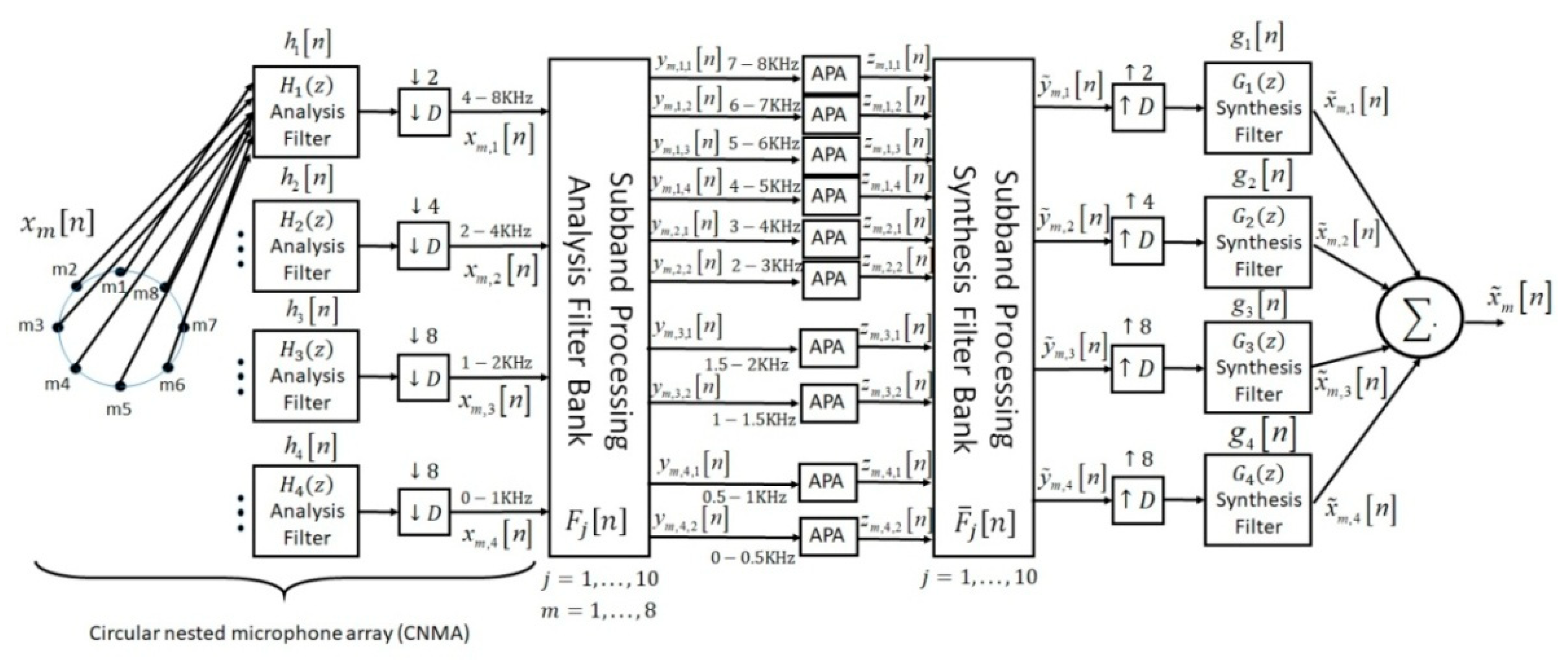
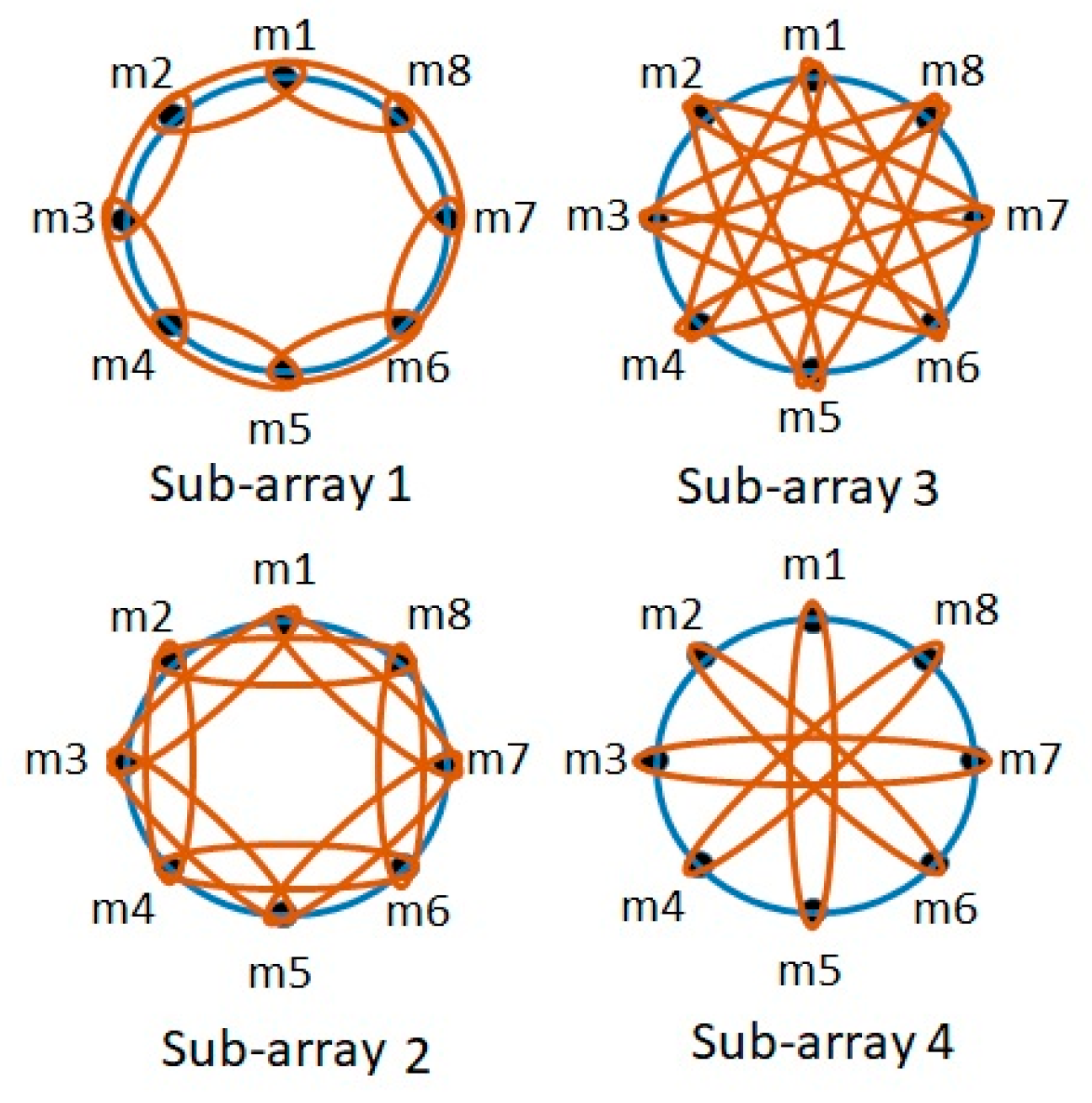
In our article, a multi-channel speech enhancement method is introduced based on the proposed circular nested microphone array in combination with the sub-band affine projection algorithm (CNMA-SBAPA). A nested microphone array increases the accuracy of the speech enhancement methods by increasing the information. Nevertheless, spatial aliasing is one of the challenges when microphone arrays are used. Firstly, a uniform circular nested microphone array (CNMA) is proposed for eliminating the spatial aliasing. Additionally, the array dimensions are designed in a way to be applicable in the real conditions. The speech components are variable in frequency bands. Therefore, a sub-band processing method is considered for speech signals. This method provides the high frequency resolution in low speech frequency components. Finally, the affine projection algorithm (APA), as an adaptive method for the speech enhancement, is implemented on sub-band signals from the circular nested microphone array (NMA). Since each APA block is implemented on a sub-band with specific information, the accuracy and speed of convergence are increased in this condition. In the last step, the synthesis filters are used to generate the enhanced speech signal. The proposed system with sub-band APA is compared by the quantitative (segmental SNR), qualitative (PESQ, MOS, and STOI) criteria, and speed of convergence with the least mean square (LMS), traditional APA, recursive least square (RLS), distributed multichannel Wiener filter (DB-MWF), and multichannel nonnegative matrix factorization-minimum variance distortionless response (MNMF-MVDR) algorithms on real and simulated data under white and colored noisy conditions. The results show the superiority of the proposed system in comparison with other previous works in all environmental conditions.

Section 2 shows the microphone signal model and the proposed uniform circular nested microphone array. Section 3 includes the proposed sub-band algorithm with analysis and synthesis filter banks in combination with the sub-band APA. The results on real and simulated data are discussed in Section 4. Section 5 includes some conclusions.

2. The Microphone Model and Proposed Nested Microphone Array

In this section, the microphone signal model was presented to produce the simulated data. In addition, the uniform CNMA was proposed for eliminating the spatial aliasing. Additionally, the nested subarrays and microphone combinations are introduced in this section.

2.1. Microphone Signal Model

The microphone signal modeling is an important part in the implementation of speech processing algorithms such as: speech enhancement, speaker tracking, speech recognition, etc. Two models are usually considered in this processing: ideal and real models [28]. In the ideal model, which is known as an open-space model, the received signal in a microphone place is a weakened and delayed version of the transmitted signal from the source location. The ideal model for microphone signals is expressed as:

$$x_m[n]=\frac{1}{r_m}s[n-{\tau }_m]+v_m[n],$$

(1)

where x_m[n] is the received signal in the m-th microphone, $s[n]$ is the speech source signal (transmitted signal), $r_m$ is the distance between source and m-th microphone, ${\tau }_m$ is the time delay between source and m-th microphone, and $v_m[n]$ is the additive noise in m-th microphone place. This model cannot show the real environments and close space conditions because the reverberation effect is discarded. Therefore, the real model is introduced for microphone signal simulations to provide the real environmental conditions for evaluating the speech enhancement algorithms. The real model simulates the microphone signal similar to the environmental conditions. The expression for real model is shown as:

$$x_m[n]=s[n]*{\gamma }_m[r_m,n]+v_m[n],$$

(2)

where the source signal is convolved to the room impulse response to model the real environments. In this equation, ${\gamma }_m[r_m,n]$ is the impulse response between the source and m-th microphone, which contains the attenuation factor and whole reverberation effect in the real conditions, and * denotes to the convolution operator. The simulated signals are similar to real conditions by considering this mathematical real model.

2.2. The Proposed Uniform Circular Nested Microphone Array

The microphone array increases the accuracy of the speech enhancement algorithms due to increasing the information. However, the spatial aliasing based on the inter-microphone distances destroys the recorded speech signals, and in the following, the performance of the speech enhancement algorithms. Nested microphone array has the capability to eliminate the spatial aliasing [29]. In this section, a uniform CNMA is proposed where by having a symmetrical shape, provides the same probability for all speakers around the array, and the quality of the enhanced signals are not dependent on the position of the speakers. Additionally, its small structure helps to be applicable in most of the conditions in comparison with other big arrays. Figure 1 shows the block diagram of the proposed speech enhancement algorithm, where the NMA part with its analysis filters and down-sampler blocks are shown in the left side.

The speech signal has a frequency range of [0–8000] Hz with a sampling frequency $F_s=16,000\mathrm{Hz}$. The proposed CNMA is designed for the frequency range [50–7800] Hz, which covers the wideband speech spectrum. The CNMA is structured by four subarrays. The first subarray is designed for the range B1 = [3900–7800] Hz, of central frequency $f_{c1}=5850\mathrm{Hz}.$ The inter-microphone distance ($d_{\lim }$) should be $d_{\lim }<\lambda /2$($\lambda$ is the wavelength of the highest frequency component in the related sub-band) to avoid the spatial aliasing, this is $d_{\lim (1)}<2.2\mathrm{cm}$ for the first subarray. The second subarray covers the frequency range B2 = [1950–3900] Hz with a central frequency of $f_{c2}=2925\mathrm{Hz}$, therefore $d_{\lim (2)}=2d_1<4.4\mathrm{cm}.$ The third subarray is defined for the frequency range B3 = [975–1950] Hz with a central frequency of $f_{c3}=1462\mathrm{Hz}$ and $d_{\lim (3)}=4d_1<8.8\mathrm{cm}$. Finally, the forth subarray is designed for the frequency range B4 = [50–975] Hz with a central frequency of $f_{c4}=512\mathrm{Hz}$ and the inter-microphone distance is $d_{\lim (4)}=8d_1<17.6\mathrm{cm}$. For a more complexity system, a higher number of microphones could be considered to design a larger nested microphone array.

Table 1. The information to design the proposed uniform CNMA.

Band	Bandwidth	Analysis Filter Bank	fc	dlim
1	B1 = [3900–7800] Hz	B1,1 = [6825–7800] Hz B1,2 = [5850–6825] Hz B1,3 = [4875–5850] Hz B1,4 = [3900–4875] Hz	5850 Hz	<2.2 cm
2	B2 = [1950–3900] Hz	B2,1 = [2925–3900] Hz B2,2 = [1950–2925] Hz	2925 Hz	<4.4 cm
3	B3 = [975–1950] Hz	B3,1 = [1425–1950] Hz B3,2 = [975–1425] Hz	1462 Hz	<8.8 cm
4	B4 = [50–975] Hz	B4,1 = [512–975] Hz B4,2 = [50–512] Hz	512 Hz	<17.6 cm

shows the summarized information to design the uniform CNMA.

The microphone array was structured to have the closest microphone distances as $d_{sim(1)}=2.2\mathrm{cm}$ (for the simulated data) based on the designed CNMA. Therefore, the first subarray included the microphone pairs {1,2}, {2,3}, {3,4}, {4,5}, {5,6}, {6,7}, {7,8}, and {8,1}. The microphone pairs {1,3}, {3,5}, {5,7}, {7,1}, {2,4}, {4,6}, {6,8}, and {8,1} were selected for the second subarray with an inter-microphone distance of $d_{sim(2)}=4.2\mathrm{cm}.$ The third subarray has the inter-microphone distance of $d_{sim(3)}=5.6\mathrm{cm}$. Then, the microphone pairs {1,4}, {2,5}, {3,6}, {4,7}, {5,8}, {6,1}, {7,2}, and {8,3} wereconsidered for this subarray. For the last subarray, the inter-microphone distance is $d_{sim(4)}=6\mathrm{cm}$ and the microphone pairs {1,5}, {2,6}, {3,7}, and {4,8} were selected for the implementation. Given our actual microphone array, the minimum inter-microphone distance that we could have was 2.7 cm (for the real data). For this reason, we did two evaluations, one for simulated data with $d_{sim(1)}=2.2\mathrm{cm}$, as dictated by the theory, and one for real data with $d_{real(1)}=2.7\mathrm{cm}$, to match our hardware. All subarrays are shown in Figure 2, which shows the designed CNMA with its small shape.

Each subarray needs an analysis filter bank to avoid the spatial aliasing and imaging. Figure 1 (left and right sides) shows the analysis and synthesis filter banks along with the up-sampler and down-sampler blocks. The multirate sampling by the use of up-samplers and down-samplers is implemented to provide the frequency bands. As shown in Figure 3a, the analysis filter bank $H_i(z)$ and down-sampler $D_i$ are realized as a multi-level tree structure. Each stage of the tree requires a high-pass filter (HPF) $H{P}_i(z)$, a low-pass filter (LPF) $L{P}_i(z),$ and a down-sampler $D_i$ (for the analysis filter bank) or up-sampler $D_i$ (for the synthesis filter bank). The relation between the analysis filter bank $H_i(z),$ the LPFs, and HPFs in the tree structure is expressed as:

$$\begin{array}{l}{H}_1(z)=H{P}_1(z)\\ H_2(z)=L{P}_1(z)H{P}_2(z^2)\\ H_3(z)=L{P}_1(z)L{P}_2(z^2)H{P}_3(z^4)\\ H_4(z)=L{P}_1(z)L{P}_2(z^2)L{P}_3(z^4).\end{array}$$

(3)

The synthesis filters $G_i(z)$ are the mirror image of analysis filters $H_i(z),$ which are implemented by the tree structure as seen in Figure 3b.

In each level of the tree, a 52-tap finite impulse response (FIR) LPF and HPF are implemented by the Remez method. The parallel filters have a stop-band attenuation of 50 dB and a transition band 0.0575. Figure 4 shows the frequency response for the analysis filter banks.

3. The Proposed Multiresolution Sub-band-APA for the Speech Enhancement

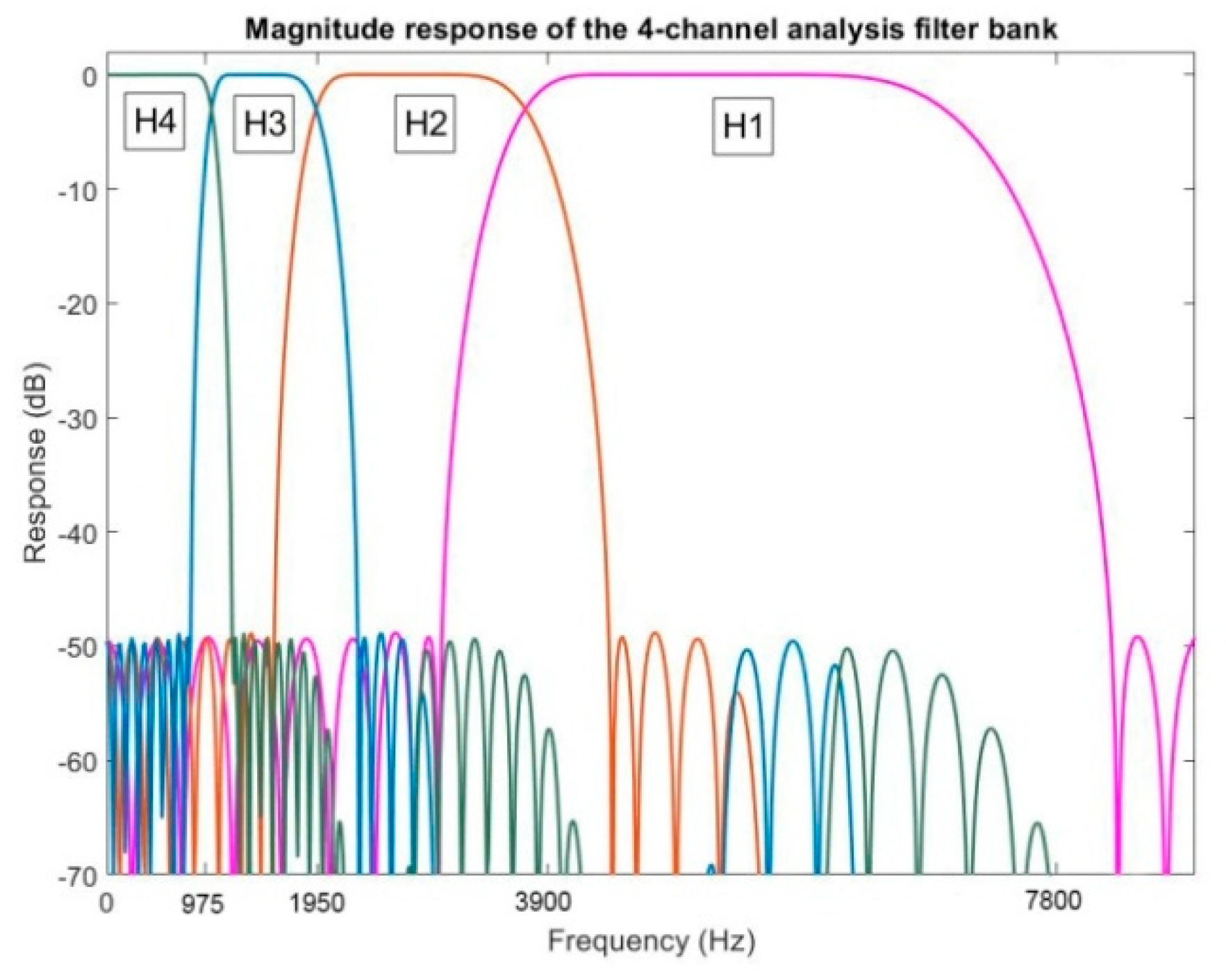
Speech is a wideband and non-stationary signal, where each frequency band has different information. This feature for the speech signal provides the conditions to evaluate the speech spectrum components by considering different frequency resolution. For example, speech information is condensed at the lower part of the spectrum. Therefore, the accuracy of the speech enhancement algorithm is increased by a focus to low frequency components. In this article, a specific sub-band processing along with a filter bank was proposed for paying more attention to lower frequencies by the use of filters with narrower bandwidths.

Table 2. The required information to design the analysis filter bank for sub-band processing in the proposed CNMA-SBAPA algorithm.

Filters	Bandwidth (Hz)	fmin (Hz)	fmax (Hz)	Filter Length (Samples)
F1[n]	462	50	512	93
F2[n]	462	512	975	115
F3[n]	450	975	1425	102
F4[n]	525	1425	1950	124
F5[n]	975	1950	2925	109
F6[n]	975	2925	3900	118
F7[n]	975	3900	4875	131
F8[n]	975	4875	5850	140
F9[n]	975	5850	6825	146
F10[n]	975	6825	7800	151

shows the information to design and implement this analysis filter bank. There is still not any certain rule for selecting the number of frequency bands. Of course, by having narrower band filters in low frequencies, we have more frequency resolution, but the concern is the computational complexity. In other hands, adding each more filter means entering more microphone pairs and more calculations. Based on the experiments, this number of frequency bands prepares enough performance and acceptable level of complexity.

As seen, the filter bandwidth is smaller in low frequencies in comparison with high frequencies. This property increases the frequency resolution for low frequencies. The most important benefit in sub-band processing is the noise estimation from the silent part of the speech signal in each sub-band. Since in the proposed denoising method, the noise estimation is required as an input for the enhancement algorithm. Therefore, the more accurate and stationary noise estimation is obtained by sub-band processing of the speech signal, which increases the denoising algorithm performance. If $x_m\left[n\right]$ is considered as an input signal for the m-th microphone, the analysis filter output for the CNMA is expressed as:

$$x_{m,i}\left[n\right]=x_m\left[n\right]*h_i\left[n\right]\mathrm{where}\left\{m=1,\dots ,8\mathrm{and}i=1,\dots ,4\right\},$$

(4)

where $x_{m,i}\left[n\right]$ is the analysis filter output and $h_i\left[n\right]$ is the impulse response for this filter. Therefore, the spatial aliasing is eliminated from each microphone pairs of CNMA by the use of analysis filters, which are designed specifically for each subarray. In the following, the microphone signals are entered to the proposed analysis filter bank for the sub-band processing. As shown in Table 2, each microphone signal is divided into 10 sub-bands. These numbers of sub-bands were selected based on our experiments in order to provide a proper efficiency and with low computational complexity, by preparing a high frequency resolution in low frequencies. Therefore, the output of the proposed analysis filter bank is expressed as:

$$y_{m,i,j}\left[n\right]=x_{m,i}\left[n\right]*F_j\left[n\right]\mathrm{where}\left\{j=1,\dots ,10,i=1,\dots ,4,m=1,\dots ,8\right\},$$

(5)

where $F_j\left[n\right]$ is the impulse response for each sub-band filter in the analysis filter bank and $y_{m,i,j}\left[n\right]$ is the output of the analysis filter bank for the j-th sub-bands and m-th microphone. The signals $y_{m,i,j}\left[n\right]$ are the sub-band microphone signals for the proposed sub-band-APA algorithm. In the following, the sub-band-APA (SBAPA) algorithm along with the circular nested microphone array (CNMA-SBAPA) is proposed for the speech enhancement. Adaptive filters as an important tool in digital signal processing have been utilized for many years in such application as: speech signal enhancement, system identification, localization and tracking, etc. In adaptive filters, the coefficients change periodically to be adapted based on the time varying features of the noise, and this property increases the performance of the denoising system in comparison with normal methods. In addition, these filters are non-linear and homogeneous since their features are dependent on the input signal. The adaptive filters have the following advantages: low delay and better tracking in non-stationary conditions [30]. These advantages are very important in dereverberation, denoising, time delay estimation, channel equalization, and speaker tracking applications. In these applications, low delay and robustness against of non-stationary noisy and reverberant conditions are important parameters to improve the performance of the proposed systems. The existence of the reference signal, which is hidden in the filter coefficient estimations, defines the system performance. 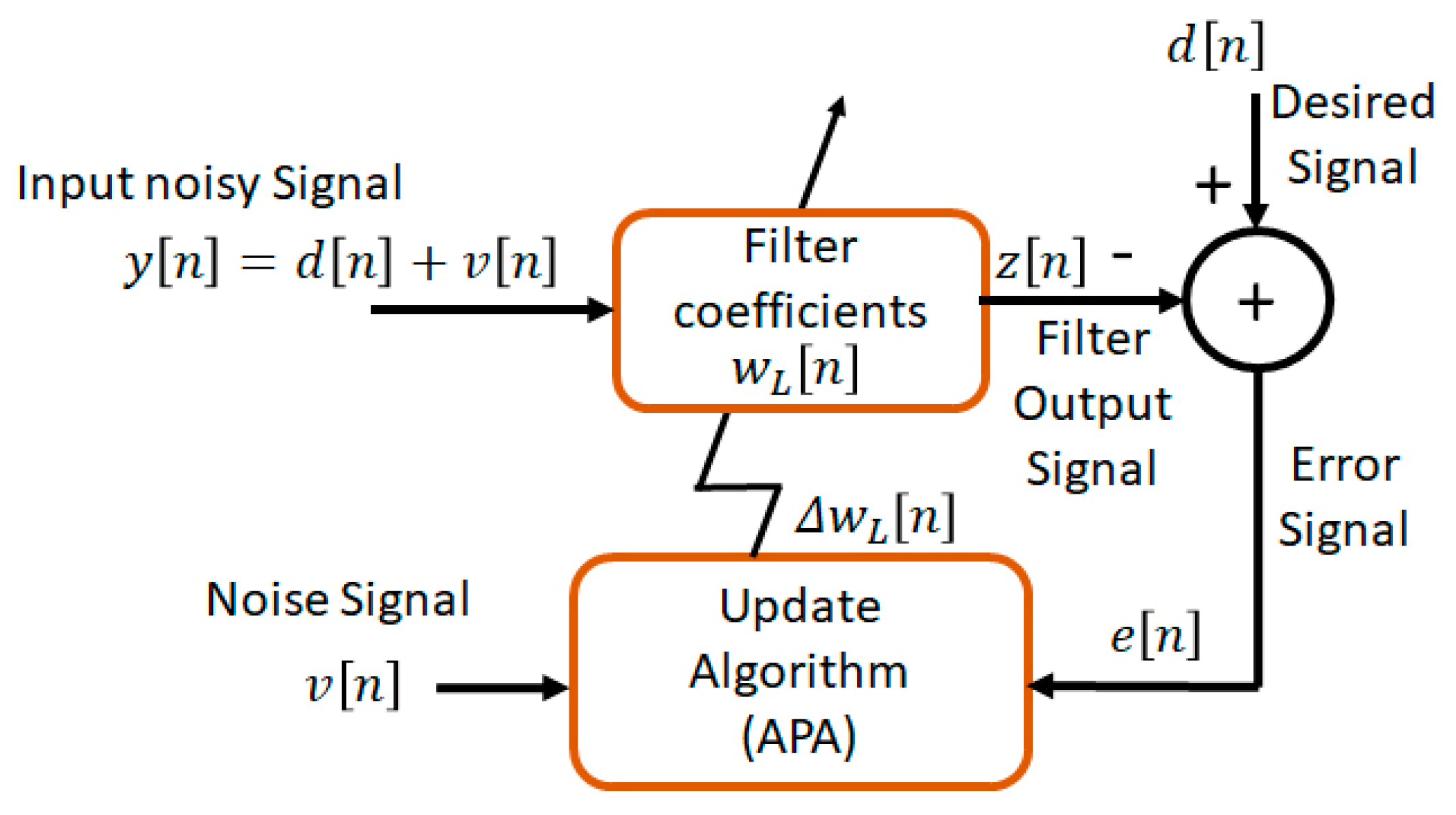Figure 5 shows the general structure of the adaptive filter in denoising applications.

We change the notation for input signal in adaptive filter ($y_{m,i,j}\left[n\right]$) to $y\left[n\right]$ for simplifying the mathematical expressions. An adaptive filter is expressed as follows [31]:

$$z\left[n\right]=w_L\left[n\right]*y\left[n\right],$$

(6)

where n is the time index, $z\left[n\right]$ is the adaptive filter output, and $w_L\left[n\right]$ is the adaptive filter coefficients with length L. The update algorithm in Figure 5 is considered as a principal part for an adaptive filter, which is the APA in this article. The main idea for an adaptive filter is to minimize the error signal $e\left[n\right]$ to make the output of the filter as similar as the desired signal.

The input signal $y\left[n\right]$ for the adaptive filter is considered as the summation of the noise (v[n]) and desired signal (d[n]), which is described as:

$$y\left[n\right]=d\left[n\right]+v\left[n\right].$$

(7)

The adaptive filter has a FIR structure, namely the filter is designed based on the limited number of coefficients in the time domain. For a filter with order of L, the filter coefficients are defined as:

$$w_L\left[n\right]=\left[w\left[0\right],w\left[1\right],\dots ,w\left[L-1\right]\right].$$

(8)

The error signal or cost function is defined as the difference between estimated and desired signal, namely:

$$e\left[n\right]=d\left[n\right]-z\left[n\right].$$

(9)

As shown in Equation (6), the output of the adaptive filter $z\left[n\right]$ is defined as the convolution between the filter coefficients $w_L\left[n\right]$ and the input signal $y\left[n\right]$, where $y\left[n\right]$ is considered as the input of the adaptive filter, namely:

$$y\left[n\right]=\left[y\left[n\right],y\left[n-1\right],\dots ,y\left[n-L\right]\right].$$

(10)

In addition, the adaptive filter coefficients change during the time, which is written as:

$$w_L\left[n\right]=w_L\left[n-1\right]+\Delta w_L\left[n\right],$$

(11)

where $\Delta w_L\left[n\right]$ is defined as the correction factor for the filter coefficients. The adaptive filter produces the correction factor based on the input and error signal. In Figure 5, several algorithms can be considered for updating the filter coefficients. The APA is one of the fastest and most efficient methods for this purpose. The AP algorithms were introduced to improve the speed of convergence in the gradient-based algorithms, especially when the input signal has a non-stationary spectrum. It is because the speed of convergence is decreased in the case of non-stationary and constraint spectrums [30].

Filter update equation is one of the most important features in the AP algorithms, which uses N vectors of the input data to update the filter coefficients instead of using one vector of the input data, i.e., the normalized least mean square (NLMS). Therefore, more information was considered in the time for accurately updating the filter coefficients. Thus, the AP algorithm is known as an improved and extended version of the NLMS method or it can be expressed mathematically as a constraints minimization problem, which is expressed as follows.

The variation for L filter coefficients during the two consecutive times is given by:

$$\Delta w_L\left[n\right]=w_L\left[n\right]-w_L\left[n-1\right].$$

(12)

We minimized Equation (13) under N constraints, which are shown in Equation (14) to extend the adaptive filter algorithm.

$${\Vert \Delta w_L\left[n\right]\Vert }^2=\Delta w_{{}_L}^T\left[n\right]\Delta w_L\left[n\right],$$

(13)

where N constraints are defined as follows:

$$w_{{}_L}^T\left[n\right]y\left[n-k\right]=d\left[n-k\right] for k=0,\dots ,N-1,$$

(14)

where $y\left[n-k\right]$ is the vector of N last sample from the input signal and $d\left[n\right]$ is the desired signal, see Figure 5. The proposed solution formulates the update algorithm for AP, which is expressed as:

$$w_L\left[n\right]{=w}_L\left[n-1\right]+A^T\left[n\right]{\left(A\left[n\right]A^T\left[n\right]\right)}^{-1}{e}_N\left[n\right],$$

(15)

where:

$$A\left[n\right]={\left(y_L\left[n\right],y_L\left[n-1\right],y_L\left[n-2\right],\dots ,y_L\left[n-N+1\right]\right)}^T,$$

(16)

and $e_N\left[n\right]$ is a vector of size $N\times 1,$ which is written as:

$$e_N\left[n\right]=d_N\left[n\right]-A\left[n\right]w_L\left[n-1\right].$$

(17)

The vector $d_N\left[n\right]$ is the desired signal with size $N\times 1,$ namely:

$$d_N\left[n\right]={\left(d\left[n\right],d\left[n-1\right],\dots ,d\left[n-N+1\right]\right)}^T.$$

(18)

The general format for AP algorithm is obtained by rewriting Equation (15) as:

$$w_L\left[n\right]{=w}_L\left[n-1-\alpha \left(N-1\right)\right]+\mu A_{{}^{\tau }}^T\left[n\right]{\left(A_{\tau }\left[n\right]A_{{}^{\tau }}^T\left[n\right]+\delta I\right)}^{-1}{e}_{N\tau }\left[n\right].$$

(19)

If $e_{N\tau }\left[n\right]$ is considered as $e_{N\tau }\left[n\right]=d_{N\tau }\left[n\right]-A_{\tau }{w}_L\left[n-1-\alpha \left(N-1\right)\right]$, then:

$$A_{\tau }\left[n\right]={\left(y_L\left[n\right],y_L\left[n-\tau \right],\dots ,y_L\left[n-(N-1)\tau \right]\right)}^T,$$

(20)

and the signal $d_{N\tau }\left[n\right]$ is expressed as:

$$d_{{}_{N\tau }}^T\left[n\right]=\left(d\left[n\right],d\left[n-\tau \right],\dots ,d\left[n-(N-1)\tau \right]\right).$$

(21)

As shown in Equation (19), the N required vectors to update the adaptive filter are not necessarily to be the last data vectors. Therefore, several versions of AP algorithms are defined based on the way to select the input data and parameters in Equation (19). There are some developed algorithms based on these parameters selections such as: the NLMS along with the orthogonal correction factor (OCF-NLMS) [32], the partial rank affine projection algorithm (PRAPA) [33], and the standard APA [34] whose parameters are $\alpha =0,\delta =0,\tau =1$. If $\delta$ parameter differs to 0, the APA algorithm is extended to APA with regularization (R-APA) [35], where the update equation for the filter coefficients is a specific case of the Levenberg Marquardt regularized APA (LMR-APA) algorithm [36].

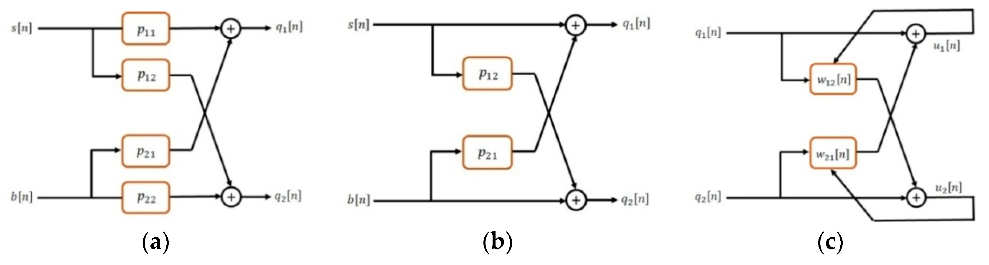
The introduced AP algorithm contains one input signal. Since pairs of microphones are used in the proposed CNMA, the AP algorithm is generalized to a two-microphone version [37]. Firstly, the generalization of a two-microphone structure is defined, where each microphone contains the mixing speech and noise signal, which is expressed as (see Figure 6a):

$$q_m\left[n\right]={\displaystyle \sum _{i=1}^2{\displaystyle \sum _{r=1}^{L-1}{p}_{im}\left[r\right]s_i\left[n-r\right]},m=1,2,}$$

(22)

where $s_i\left[n\right]$ represents the source signals, $q_m\left[n\right]$ is the microphone signals, L is the impulse response length, and $p_{im}\left[r\right]$ are the impulse responses between the microphone and sources. These impulse responses are considered as linear time-invariant (LTI) systems. Two source signals $s_i\left[n\right]$ are selected as the speech signal $s\left[n\right]$ and noise signal $b\left[n\right]$. It is assumed that the speech and noise signals are independent, which means $E\left\{s\left[n\right]b\left[n-m\right]\right\}=0,\forall m,$ where E denotes to expected value. Then, the noise and speech signals are uncorrelated. Based on the general structure, which is shown in Figure 6a, the microphone signals $q_1\left[n\right]$ and $q_2\left[n\right]$ are expressed as follows:

$$q_1\left[n\right]=s\left[n\right]*p_{11}+b\left[n\right]*p_{21},$$

(23)

$$q_2\left[n\right]=s\left[n\right]*p_{12}+b\left[n\right]*p_{22}.$$

(24)

In addition, $p_{11}$ and $p_{22}$ represent the impulse responses for direct path, and $p_{12}$ and $p_{21}$ are cross-coupling for the channels between the sources and microphones. The presented model is simplified by considering $p_{11}=p_{22}=\delta \left[n\right],$ which is shown in Figure 6b as:

$$q_1\left[n\right]=s\left[n\right]+b\left[n\right]*p_{21},$$

(25)

$$q_2\left[n\right]=s\left[n\right]*p_{12}+b\left[n\right].$$

(26)

Therefore, the microphone signals are generated based on the impulse responses between the source and microphones, noise, and speech signals. The structure in Figure 6c was proposed to retrieve the source signal from the received noisy signals $q_1\left[n\right]$ and $q_2\left[n\right]$. The proposed structure provides the conditions to retrieve the original signal by the use of adaptive filters $p_{11}$ and $p_{22}$. The signals $u_1\left[n\right]$ and $u_2\left[n\right]$ for the two-microphone structure are defined as follows:

$$u_1\left[n\right]=q_1\left[n\right]-q_2\left[n\right]*w_{21}\left[n\right],$$

(27)

$$u_2\left[n\right]=q_2\left[n\right]-q_1\left[n\right]*w_{12}\left[n\right],$$

(28)

where in Equations (27) and (28), $w_{12}\left[n\right]$ and $w_{21}\left[n\right]$ are the adaptive filters for eliminating the noise of microphone signal $q_1\left[n\right]$ and the speech of microphone signal $q_2\left[n\right]$, respectively. Signals $u_1\left[n\right]$ and $u_2\left[n\right]$ are rewritten by replacing Equations (25) and (26) to Equations (27) and (28) as:

$$u_1\left[n\right]=s\left[n\right]*\left[\delta \left[n\right]-p_{12}*p_{21}\right]+b\left[n\right]*\left[p_{21}-w_{21}\left[n\right]\right],$$

(29)

$$u_2\left[n\right]=b\left[n\right]*\left[\delta \left[n\right]-p_{21}*p_{12}\right]+s\left[n\right]*\left[p_{12}-w_{12}\left[n\right]\right].$$

(30)

Two adaptive filters $w_{12}\left[n\right]$ and $w_{21}\left[n\right]$ are required to retrieve the original speech signal from the noisy signals $u_1\left[n\right]$ and $u_2\left[n\right]$. There is just a unique structure for adaptive filters $w_{12}\left[n\right]$ and $w_{21}\left[n\right]$ as $w_{12}\left[n\right]=p_{12}$ and $w_{21}\left[n\right]=p_{21}$ to retrieve the enhanced speech of noisy signals $u_1\left[n\right]$ and $u_2\left[n\right]$. This structure requires a VAD for preparing the noise estimation from the silent part of the recorded signals.

The AP algorithm is generalized to a two-microphone structure based on the obtained Equation (19) for updating the filter coefficients. The AP algorithm is the generalized version of the two-microphone NLMS [38], which is shown in Figure 6c for adaptive speech enhancement algorithm. Therefore, the adaptive filter coefficients $w_{12}\left[n\right]$ and $w_{21}\left[n\right]$ for two-microphone APA are expressed as:

$$w_{12}\left[n\right]=w_{12}\left[n-1\right]+\frac{{\mu }_{12}}{q_1\left[n\right]q_1{\left[n\right]}^T+\delta I}{q}_1\left[n\right]u_2\left[n\right],$$

(31)

$$w_{21}\left[n\right]=w_{21}\left[n-1\right]+\frac{{\mu }_{21}}{q_2\left[n\right]q_2{\left[n\right]}^T+\delta I}{q}_2\left[n\right]u_1\left[n\right],$$

(32)

where $q_1\left[n\right]$ and $q_2\left[n\right]$ are defined as $q_1\left[n\right]=\left[q_1\left[n\right],q_1\left[n-1\right],\dots ,q_1\left[n-N+1\right]\right]$ and $q_2\left[n\right]=\left[q_2\left[n\right],q_2\left[n-1\right],\dots ,q_2\left[n-N+1\right]\right]$. The matrices of the two-microphone signals $q_1\left[n\right]$ and $q_2\left[n\right]$ have dimensions $L\times N,$ where L is the adaptive filter length and N is the projection order. The two parameters ${\mu }_{12}$ and ${\mu }_{21}$ are the step sizes, which control the convergence of adaptive filters $w_{12}\left[n\right]$ and $w_{21}\left[n\right]$. These parameters should be selected in the range [0,2] to assure the convergence of AP algorithm. If N is selected as 1, the AP algorithm is converted to the NLMS method.

The proposed sub-band APA not only increased the accuracy of the speech enhancement algorithm, but also the speed of convergence was improved (Table 6 in the results section) in the implementations because the noise was estimated separately for each sub-band and it was stationary on narrow bandwidths. Then, the SBAPA was implemented on generated sub-bands by the analysis filters in Figure 3. 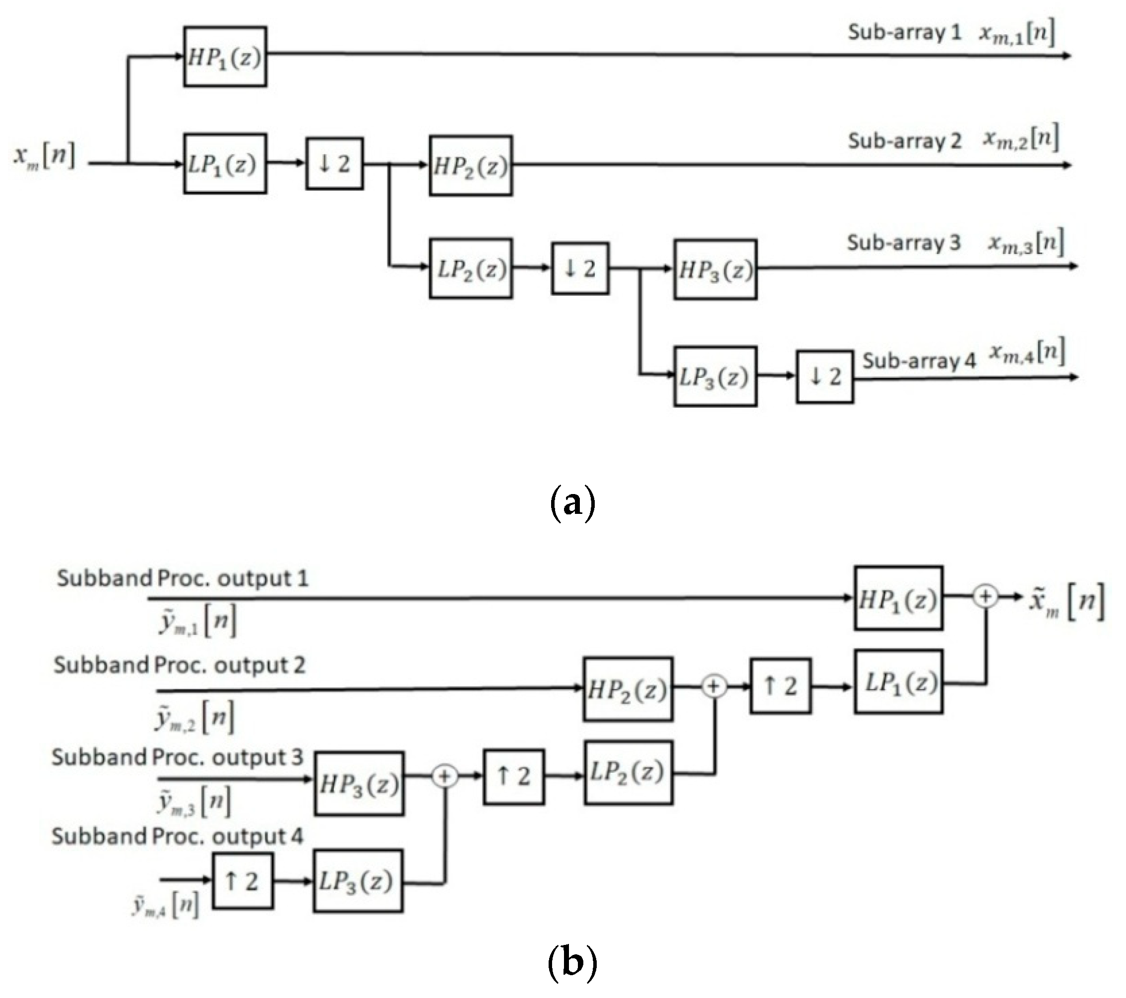As shown in Figure 1, a symmetrical synthesis filter bank and synthesis filters related to the nested microphone array were implemented for the reconstruction the final enhanced signal. The synthesis filters as similar as the analysis filters were implemented based on the tree structure in Figure 3b. Finally, all sub-band signals were summed to generate the final enhanced signal. In the next section, the performance of the proposed CNMA-SBAPA was compared with other previous works.

4. Results and Discussion

The experiments in order to evaluate the performance of the proposed method were implemented on the real and simulated data. The TIMIT dataset was considered for the simulated data, where the data collection MDAB0 by four continuous sentences SX139, SX229, SX319, and SX409 were selected as a male speaker in the simulations [39]. This dataset includes short sentences for testing and training the algorithms. The tones and frequency components are two different parameters in the speech signal. There are pitch and speech spectrum components for the speakers. It is important to work with male or female signals for the algorithms, which works with the pitch parameter. Since this parameter changes highly based on the gender. Since we consider the speech spectrum, then the issue to use the male or female speakers does not change the results. Therefore, 12.5 s male-speech signal is used for implementations and experiments. A voice activity detector is implemented to detect the silence part of the speech signal [40], and the noise spectrum is estimated of these parts for the proposed SBAPA. 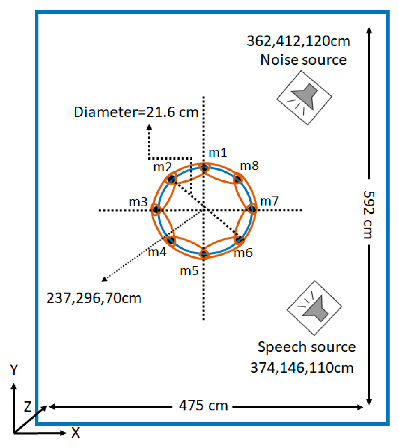Figure 7 shows the simulated room with the location of speakers and microphone array. The inter-microphone distances $d_{sim}=2.2\mathrm{cm}$ for the simulated data was selected based on the designed array. A speaker and a steered noise source were considered in the simulations. The room dimensions, speaker, and noise source locations were selected as 475,592,420cm, 374,146,110cm, and 362,412,120cm, respectively. These dimensions and locations were considered the same as the real room recording conditions. In addition, the proposed algorithm was implemented on real data to evaluate the real effect of the noise and reverberation on the performance. For this purpose, the real speech signal was recorded in the speech processing laboratory at Fondazione Bruno Kessler (FBK), Trento, Italy. 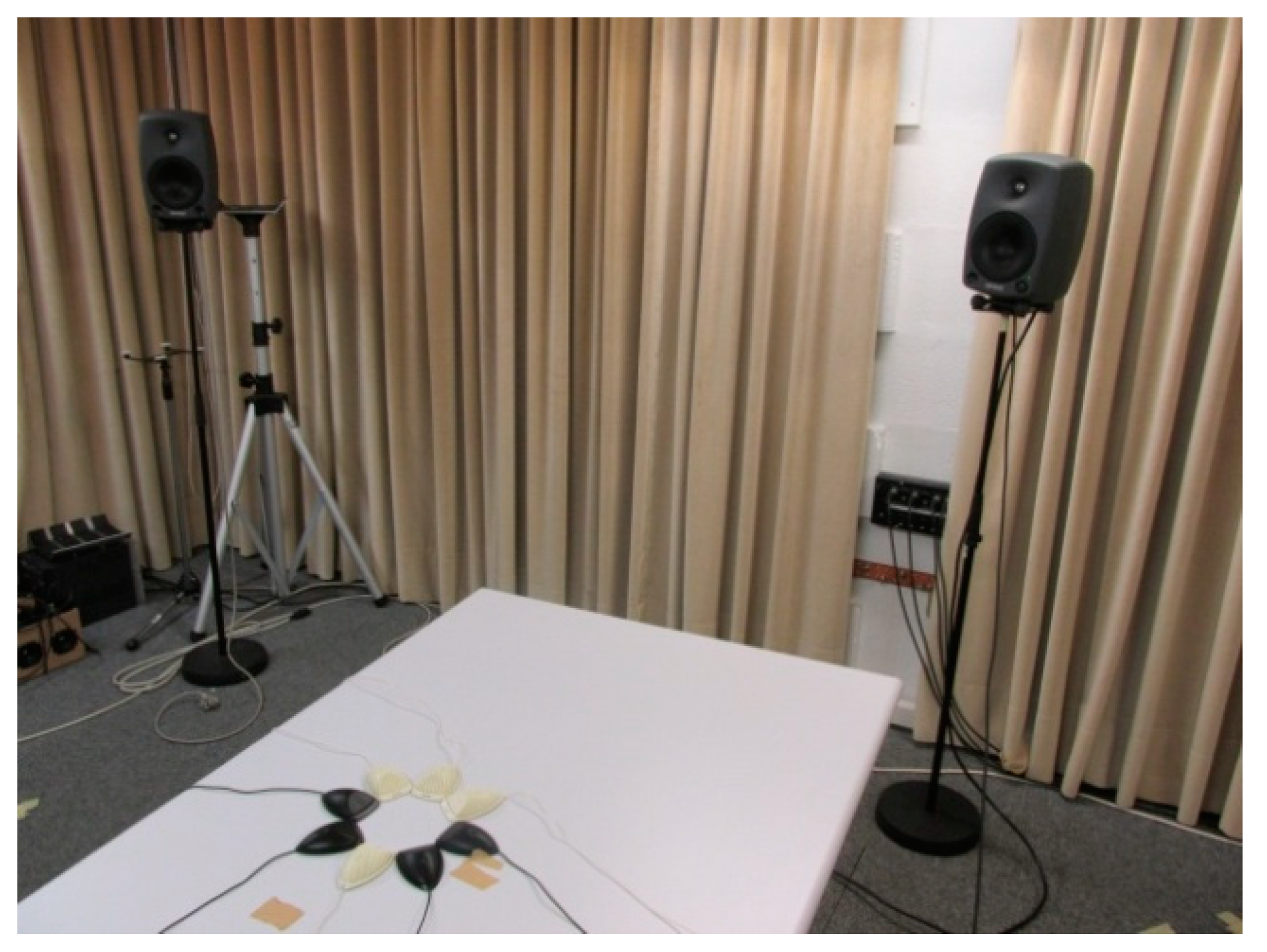Figure 8 shows a view of the recording room at FBK. Two electronic speakers were used instead of the human and noise source in the process of data recording. In addition, Figure 8 shows the position of the circular NMA in the center of the room. We were able to consider the minimum inter-microphone distance in the real conditions with our setup (see Figure 8) as $d_{real}=2.7\mathrm{cm}$ because of the microphone dimension, electronic board, and the microphone shield. Additionally, each microphone had a cross section, where in the real conditions it was about 0.7 cm. It means it is hard to measure the exact distance between two microphones and it has some errors. Since all cross sections in a microphone are areas for a sound recording, then, based on all limitations, we were forced to have this inter-microphone distance for real data implementation even with a few millimeters difference with the mathematical calculations. Therefore, the differences in the results of our proposed method for the real and simulated data were for this an issue. In the real condition, there are always some inaccuracy factors for the measurements. We found the center of the room and the microphones were located on the table based on the primary measurements. All microphones were connected to the sound recording system, which uses parallel acquisition for all microphone channels. All channel acquisitions were synchronized and there was not any delay between recorded signals in different microphones or channels. The phase error based on the recording condition was very low and was even close to zero based on the audio recording system. In the real room, the table did not make any direct reflection. All the reflected waves from the table will cross to the walls and ceiling firstly, and since all of them were covered with curtains and sound absorption panels, the indirect reflections to the microphones were very few. Both speakers were connected to the two computers for playing the speech and noise with a sampling frequency of $F_s=16,000\mathrm{Hz}$. The microphone, sound, and noise sources were selected in the simulations with exactly the same real conditions for the results to be comparable in these two conditions. 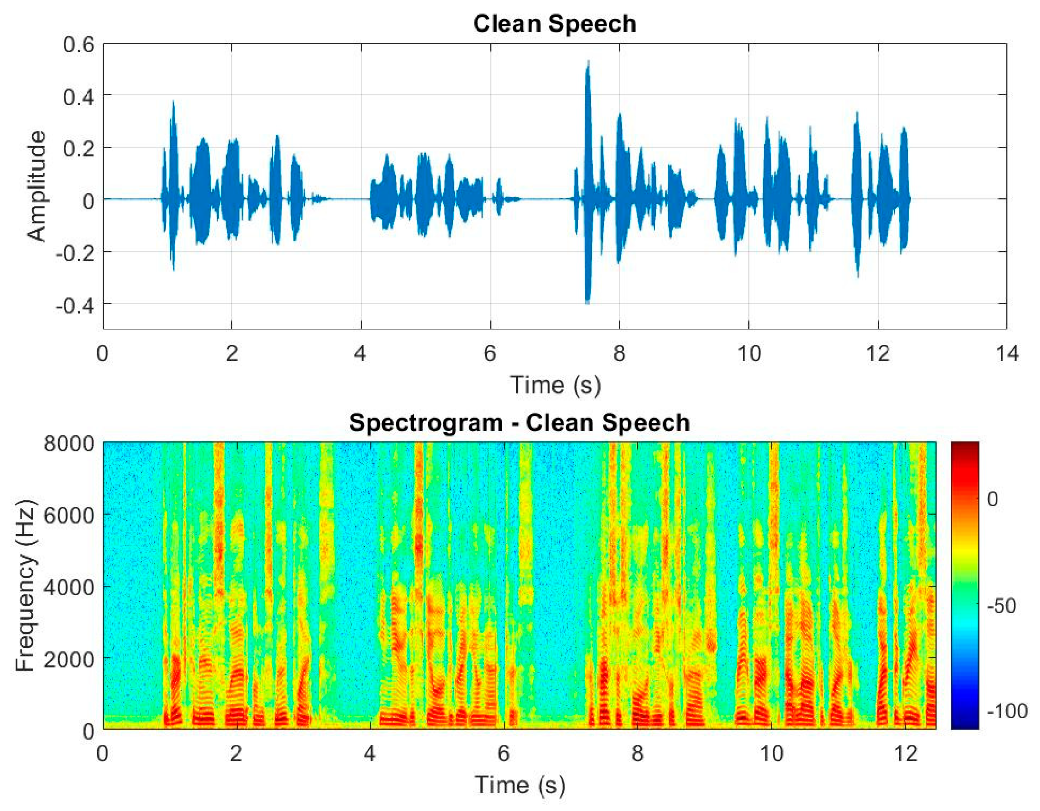Figure 9 shows the time-domain and spectrum of the male speech signal.

The reverberation effect was considered in the experiments to provide the simulation conditions similar to the real scenarios. The image model was implemented in the simulations to produce the reverberation effect similar to the real conditions [41]. The image model produced the room impulse response between the source and microphone by considering the speaker position, microphone location, sampling frequency, room dimension, room reflection coefficients, impulse response length, and reverberation time. The received signal to the microphone was simulated by the convolution between the generated impulse response by the image method and the source signal. The impulse response was generated for the noise and speech sources because both receive the same effect of the room reverberation. In addition, noise was additive with the speech signal in the microphone positions. 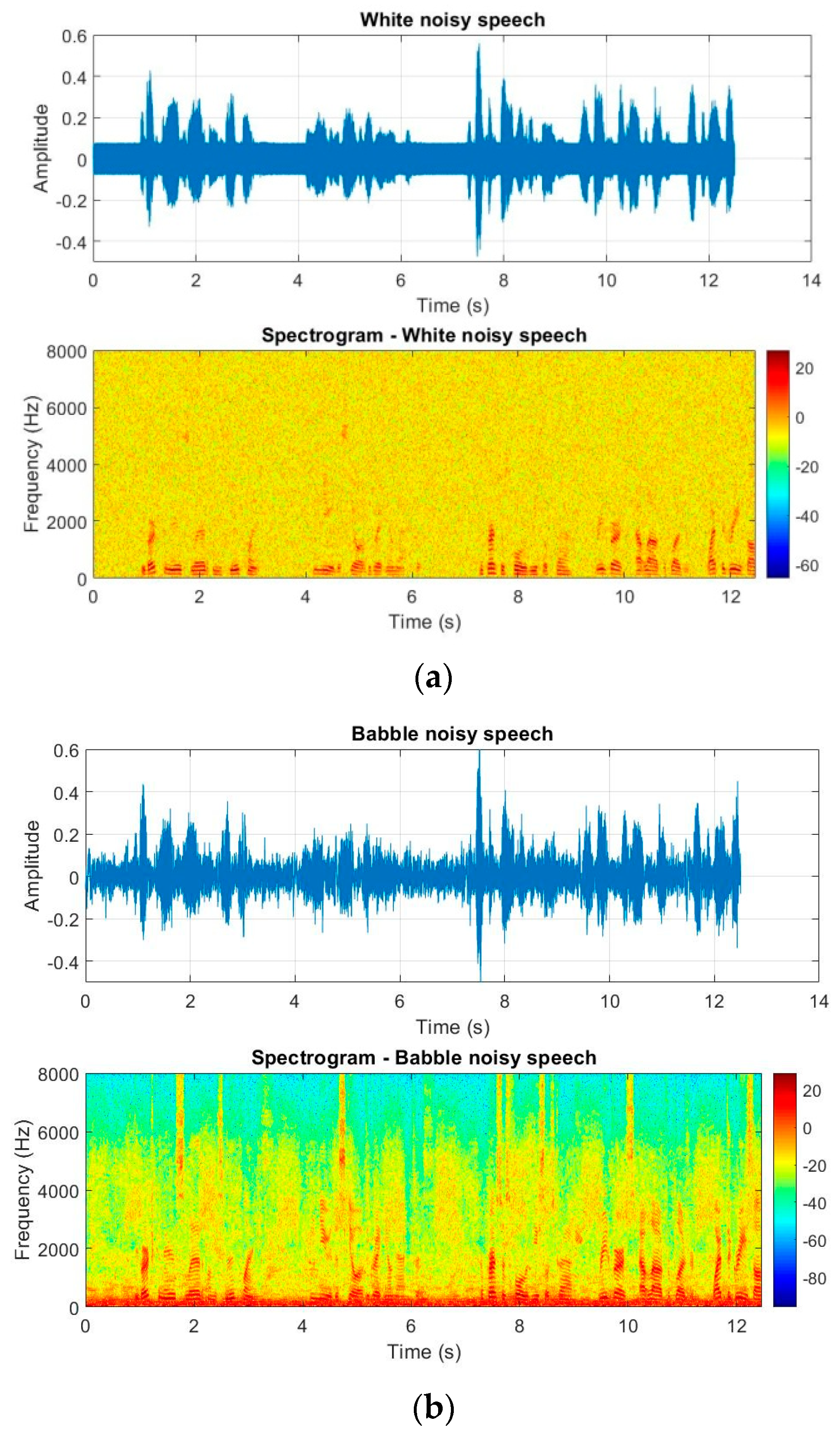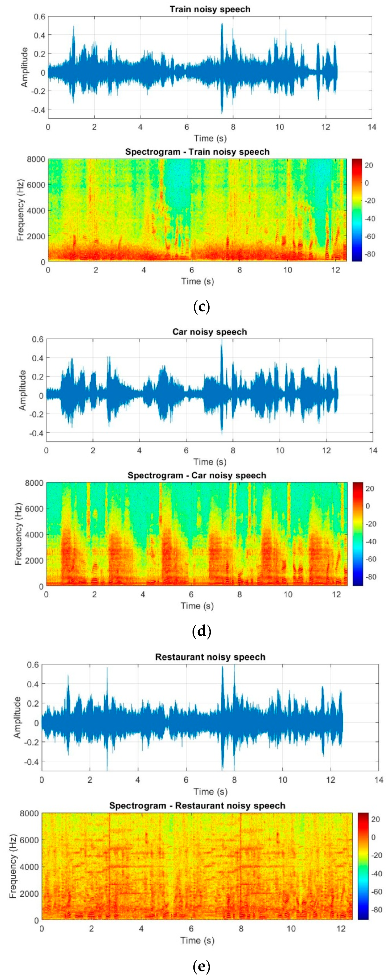The room reverberation time was selected as $R{T}_{60}=350\mathrm{ms},$ which was considered for a room with a low level of reverberation to be the same as the real conditions. To generate the noisy signal, five types of noise were considered for the simulated and real data such as white noise, babble noise, train noise, car noise, and restaurant noise. Figure 10 shows the time-domain and spectrum for these noisy signals according to a SNR = 0 dB. The noise signal duration was 12.5 s, the same as the speech signal.

The Hamming window with a length of 30 ms was selected for signal blocking to keep the stationarity of the signal in the short time. The projection order was considered as N = 4 to keep the computational complexity in an acceptable range in addition to a proper accuracy of the algorithm. Additionally, the step sizes were chosen as ${\mu }_{12}=1$ and ${\mu }_{21}=1$ to provide the fast convergence for the proposed SBAPA in the real-time implementations. The evaluations in this article were implemented by the use of MATLAB software version 2019b on a PC with processor Inter Core i7-7700k, 4.20 GHz, and with 32GB RAM to be able to implement the proposed algorithm in the real-time conditions.

The proposed SBAPA in combination with a proposed circular nested microphone array (CNMA-SBAPA) was compared with the LMS [20], traditional APA [31], RLS [21], DB-MWF [9], and MNMF-MVDR [24] algorithms. These methods were compared because all of them are based on the adaptive filters and multi-channel beamforming as a main category for comparison. There are many methods for comparison with the proposed algorithm but the comparison should be based on the common theme in implementations. Therefore, the adaptive filter-based algorithms were selected for this comparison. The qualitative and quantitative criteria were considered to show the superiority of the proposed method in comparison with other previous works. For this purpose, the SegSNR [7], PESQ [4], MOS [5], and STOI [6] criteria were selected for the comparison. The SegSNR is a quantitative criterion, which shows the improvement in the enhanced signal due to the percentage of the noise power elimination from the noisy signal, namely:

$${\mathrm{SegSNR}}_{(dB)}=\frac{1}{R}{\displaystyle \sum _{i=o}^{R}10{\log }_{10}\left(\frac{{\displaystyle \sum _{j=0}^{Q-1}{\left|S_j\left[n\right]\right|}^2}}{{\displaystyle \sum _{j=0}^{Q-1}{\left|S_j\left[n\right]-Z_j\left[n\right]\right|}^2}}VA{D}_i\right)}$$

(33)

where $S\left[n\right]$ and $Z\left[n\right]$ are the clean and enhanced speech signals, respectively. The variable Q is the mean averaging value of the SNR for the output signal. The variable R is the number of only-speech frames and $VAD$ is a speech detector, which is 1 for only-speech frames and 0 for only-noise frames. Therefore, the SegSNR is appropriate to show the speech enhancement performance. Many of the speech enhancement algorithms eliminate some part of the speech signals in addition to the noise frames, which decreases the speech perception for the enhanced signals. Then, three well-known qualitative criteria are considered in the evaluations. The first one is the PESQ, which is defined based on the standard ITU-T P.862 for qualitative evaluations of speech signals in mobile stations [4,42]. In fact, the PESQ criteria is used in the numerical representation of qualitative evaluations for enhanced speech signals. The defined range for this criteria is [−0.5 4.5], where −0.5 and 4.5 show the lowest and highest quality of the enhanced speech, respectively. Additionally, the results were compared with the MOS score criteria. These are qualitative criteria in telecommunication systems that represent the clarity, perception, and intelligibility of the enhanced signal. The MOS criteria are defined based on the standard ITU-T P.800 [5,43] in telecommunication systems. The evaluation results based on the MOS criteria was implemented by the use of some volunteers, by listening to the enhanced signal, where 1 and 5 are the lowest and highest scores in this criteria, respectively.

Table 3. The numerical scores for the mean opinion score (MOS) criteria in the evaluation process.

Rating	Quality (Standard ITU-T P.800)	Impairment
5	Excellent	Imperceptible
4	Good	Perceptible but not annoying
3	Fair	Slightly annoying
2	Poor	Annoying
1	Bad	Very annoying

shows the defined scores for the MOS criteria in the evaluations.

Finally, the last qualitative criteria for evaluations is the STOI. This criteria predicts the intelligibility of humans based on a series of cases. The speech intelligibility measurement is based on the existence of a series of pre-assumptions, but if the noisy signal is processed based on the time-frequency weighting, the final results are not trustable. The STOI is an objective intelligibility measurement, which represents the highest convolution value by the intelligibility of both noisy and weighted time-frequency noisy signals. In addition, the lowest and highest scores for the STOI criteria are 0 and 1, which represent the best and the worst enhancement performance, respectively.

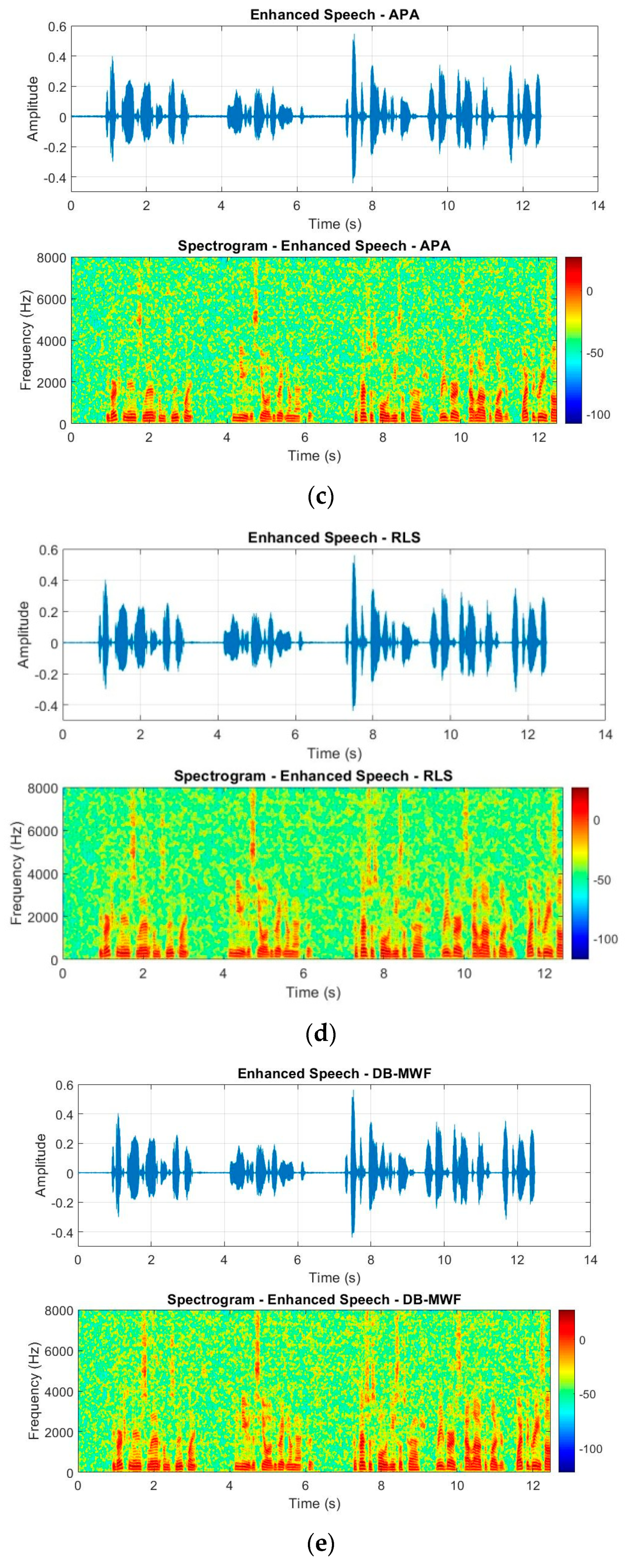
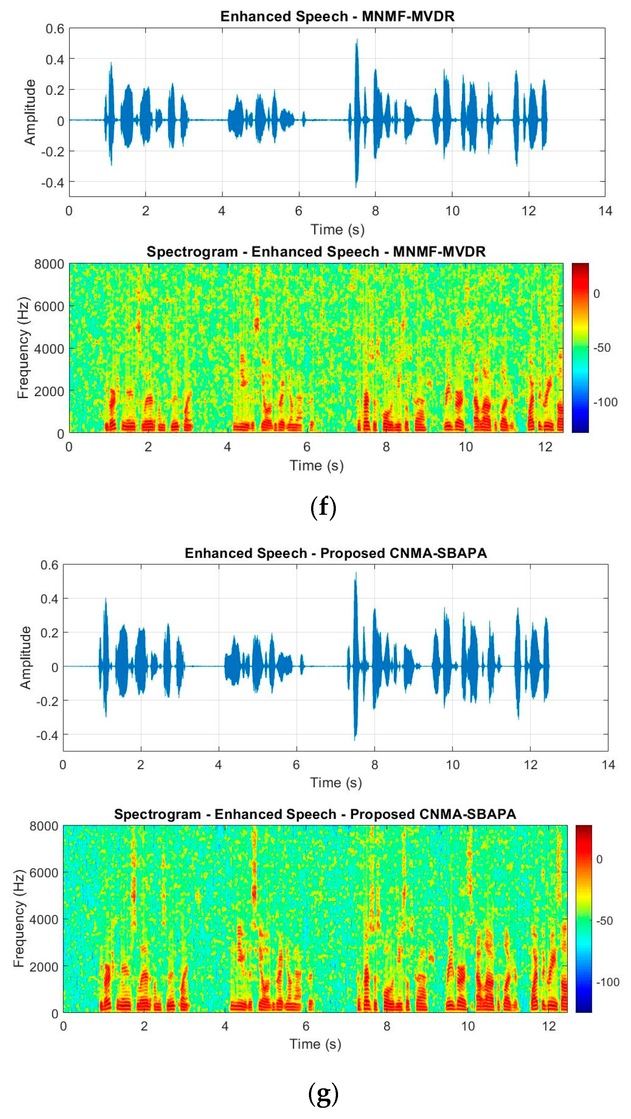
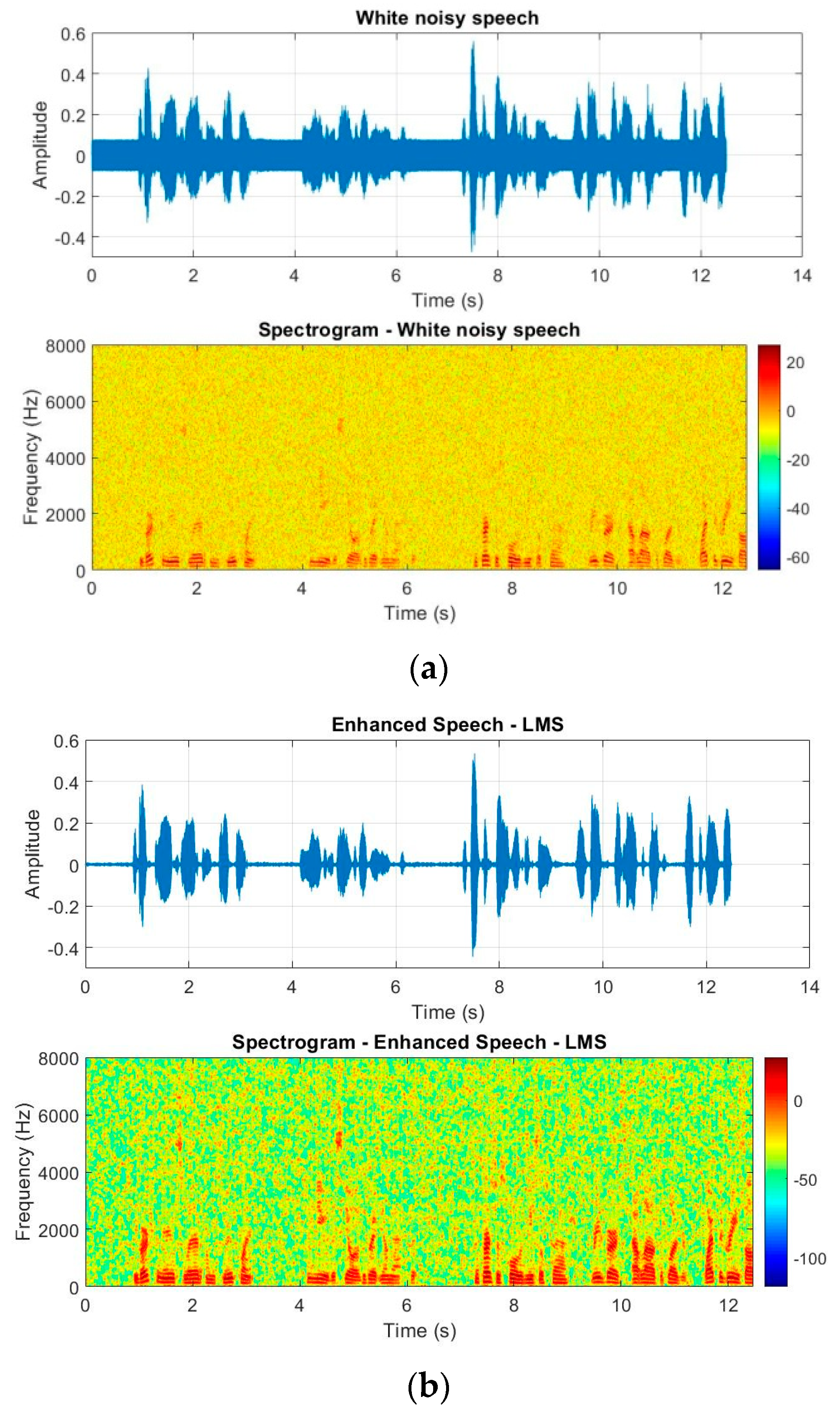
Firstly, the proposed method was evaluated on the white noise and then, the other colored noise were considered in the experiments. The proposed CNMA-SBAPA was evaluated on real and simulated data in comparison with the LMS, traditional APA, RLS, DB-MWF, and MNMF-MVDR algorithms. Figure 11 shows the time-domain and spectrum for the noisy and enhanced signals in the presence of white noise for SNR = 0 dB. As seen in these figures, the proposed CNMA-SBAPA method decreased more level of the noise with less distortion in comparison with other works. However, the numerical values are necessary for comparison. In the following, the experiments were evaluated with quantitative and qualitative criteria.

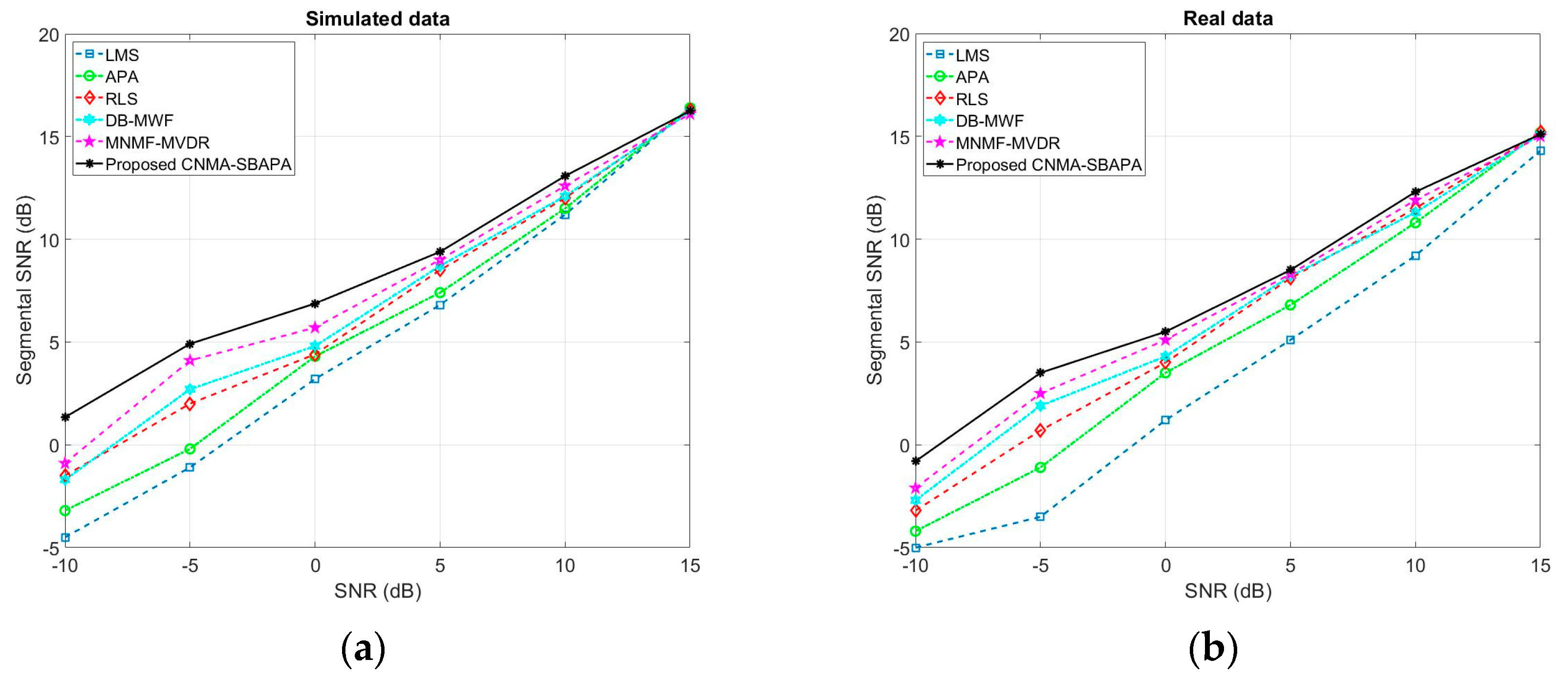
In the following, the proposed method was compared by numerical criteria with other previous works. Figure 12 shows the SegSNR results in SNRs [−10, −5, 0, 5, 10, and 15] dB for the proposed CNMA-SBAPA in comparison with the LMS, traditional APA, RLS, DB-MWF, and MNMF-MVDR for real and simulated data in the presence of white noise. As seen, the proposed method had a superior performance in different ranges of SNRs in comparison with the rest of the works, namely a better noise elimination was reached via the proposed algorithm. For example, the proposed method enhanced the noisy speech signal with SNR = −10 dB to SegSNR = 1.35 dB in comparison with SegSNR = −4.58 dB in LMS, SegSNR = −3.21 dB in APA, SegSNR = −1.57 dB in RLS, SegSNR = −1.68 dB in DB-MWF, and SegSNR = −0.94 dB in MNMF-MVDR. Nevertheless, the quantitative criteria are not enough to properly evaluate a method, and both quantitative and qualitative criteria should be considered in the evaluations.

In addition, the proposed method was compared with previous works by qualitative criteria such as the PESQ, MOS, and STOI. We used 20 volunteers, where they listened first to the clean signal by the headset to have an idea of an excellent signal with a rating of 5 in the MOS scale and a noisy signal (before enhancement), which is the worst option in the MOS scale with a rating of 1. Then, the enhanced signal in a different range of SNRs were played for them, and they were asked to select a rate between 1 and 5 based on the Table 3. 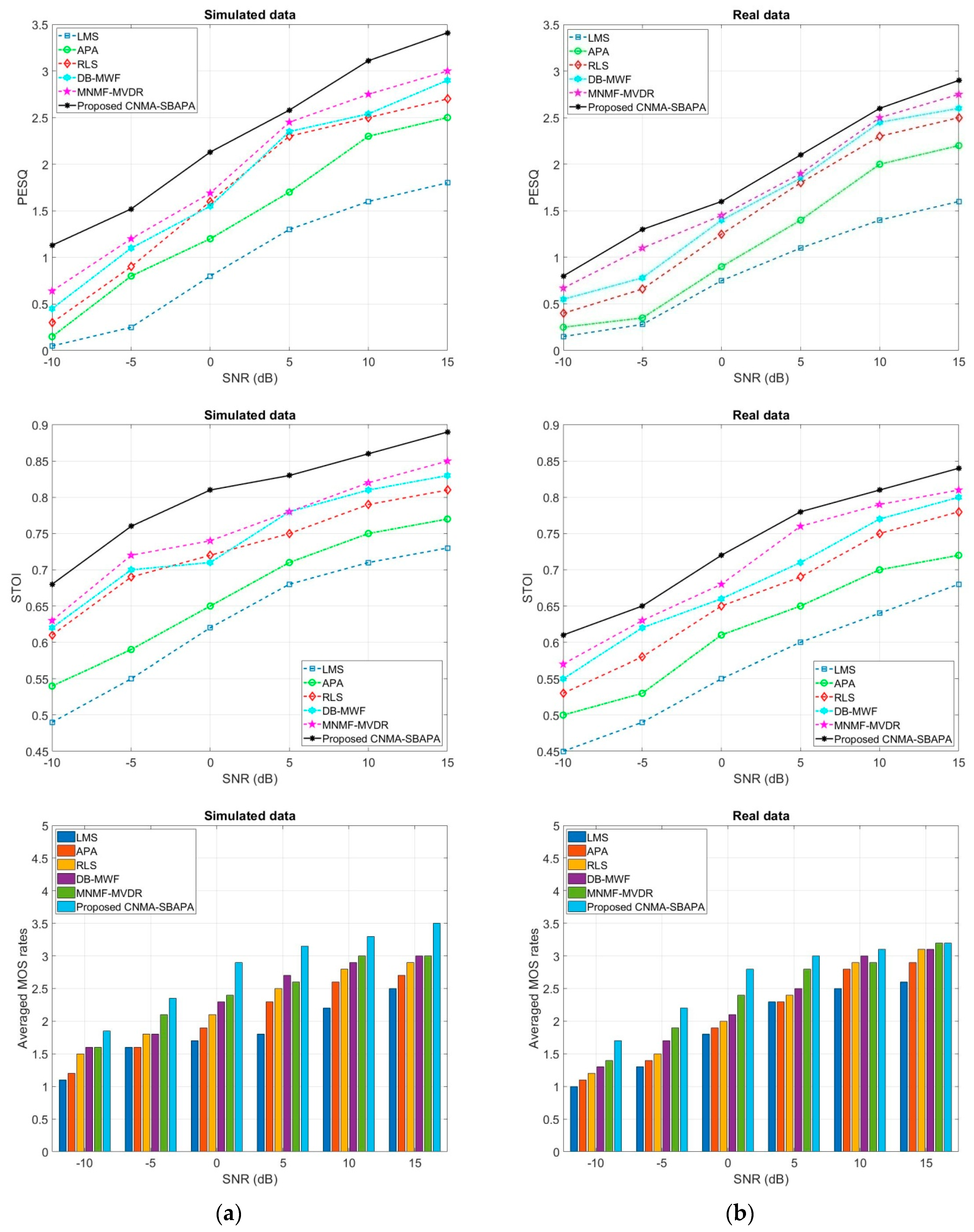Figure 13 shows the PESQ, STOI, and averaged MOS criteria for the enhanced signal by the proposed method in comparison with previous works on real and simulated data for different ranges of SNRs in the presence of white noise. As seen, the proposed method had the best performance in comparison with previous works. For example, the PESQ score was 3.41 in the proposed method in comparison to 1.82 in LMS, 2.51 in APA, 2.73 in RLS, 2.93 in DB-MWF, and 3.1 in MNMF-MVDR, for SNR = 15 dB for simulated data. In addition, the STOI criteria was 0.89 in the proposed method in comparison to 0.73 in LMS, 0.77 in APA, 0.81 in RLS, 0.83 in DB-MWF, and 0.85 in MNMF-MVDR, for SNR = 15 dB. The other criteria for comparison was the average MOS rate, which was 3.5 in the proposed method in comparison to 2.5 in LMS, 2.7 in APA, 2.9 in RLS, 3.0 in DB-MWF, and 3.0 in MNMF-MVDR, for SNR = 15 dB. Therefore, the proposed method was superior for enhancing the noisy signals by considering both quantitative (Figure 12) and qualitative (Figure 13) criteria in comparison to previous works in the presence of white noise. In addition, the proposed method was implemented on colored noises to show the reliability of the results. For this purpose, the proposed method was evaluated on babble, train, car, and restaurant noises for the real and simulated data and for SNR ranges [−10, −5, 0, 5, 10, and 15] dB.

Table 4. The comparison between PESQ, MOS, STOI, and SegSNR for the proposed CNMA-SBAPA in comparison with the LMS, traditional APA, RLS, DB-MWF, and MNMF-MVDR methods on the simulated data for colored noises such as: train, babble, car, and restaurant noises in different range of SNRs (the bold numbers are the best results).

SNR (dB)	Methods	Babble Noise				Train Noise				Car Noise				Restaurant Noise
		SegSNR	PESQ	STOI	MOS	SegSNR	PESQ	STOI	MOS	SegSNR	PESQ	STOI	MOS	SegSNR	PESQ	STOI	MOS
	LMS	−5.23	0.34	0.44	1.10	−5.74	0.29	0.41	1.05	−6.25	0.25	0.36	1.05	−6.87	0.18	0.37	1.00
−10	APA	−4.63	0.63	0.51	1.15	−5.15	0.56	0.47	1.10	−5.96	0.48	0.43	1.05	−6.08	0.52	0.39	1.10
	RLS	−2.91	0.86	0.58	1.45	−3.29	0.81	0.51	1.35	−3.98	0.74	0.48	1.30	−4.61	0.65	0.44	1.30
	DB-MWF	−2.48	0.92	0.57	1.55	−3.08	0.89	0.53	1.45	−3.46	0.78	0.50	1.45	−4.77	0.79	0.47	1.40
	MNMF-MVDR	−2.23	1.04	0.60	1.60	−2.83	0.96	0.56	1.50	−3.29	0.85	0.53	1.55	−4.29	0.84	0.48	1.45
	CNMA-SBAPA	−1.71	1.19	0.65	1.85	−2.09	1.16	0.63	1.70	−2.69	1.03	0.59	1.65	−3.14	0.99	0.56	1.60
	LMS	−2.66	0.48	0.53	1.50	−3.02	0.44	0.51	1.40	−3.59	0.39	0.46	1.35	−3.78	0.41	0.47	1.35
−5	APA	−1.89	0.76	0.59	1.55	−2.13	0.68	0.56	1.45	−2.41	0.61	0.51	1.40	−3.26	0.65	0.54	1.4
	RLS	0.57	0.91	0.65	1.75	−0.08	0.82	0.62	1.70	−1.14	0.79	0.58	1.60	−1.97	0.72	0.60	1.55
	DB-MWF	1.18	0.98	0.67	1.90	0.81	0.94	0.62	1.80	−0.35	0.87	0.60	1.65	−0.29	0.93	0.59	1.70
	MNMF-MVDR	1.97	1.13	0.68	1.95	1.36	1.06	0.65	1.95	0.87	1.03	0.61	1.75	0.96	0.98	0.61	1.70
	CNMA-SBAPA	3.63	1.43	0.73	2.30	3.06	1.36	0.70	2.20	2.73	1.32	0.68	2.15	2.26	1.20	0.64	2.10
	LMS	3.58	0.75	0.61	1.65	3.13	0.66	0.56	1.55	2.69	0.59	0.52	1.5	2.24	0.54	0.49	1.55
0	APA	4.07	1.14	0.63	1.8	3.75	1.05	0.61	1.70	3.21	0.99	0.57	1.65	3.56	0.93	0.55	1.65
	RLS	4.12	1.53	0.71	2.05	3.98	1.47	0.66	1.95	3.67	1.41	0.64	1.9	3.92	1.36	0.62	1.85
	DB-MWF	4.83	1.61	0.72	2.25	4.39	1.59	0.68	2.00	3.98	1.58	0.66	1.95	4.11	1.49	0.65	1.95
	MNMF-MVDR	5.07	1.72	0.75	2.35	4.56	1.67	0.7	2.25	4.31	1.69	0.69	2.15	4.39	1.61	0.65	2.10
	CNMA-SBAPA	5.40	2.04	0.78	2.85	5.13	1.98	0.75	2.70	4.95	1.91	0.73	2.65	4.78	1.84	0.75	2.55
	LMS	8.59	1.22	0.67	1.75	8.46	1.14	0.64	1.70	8.25	1.09	0.60	1.7	8.17	1.01	0.57	1.65
5	APA	8.96	1.63	0.69	2.20	8.74	1.57	0.66	2.15	8.39	1.5	0.63	2.05	8.22	1.46	0.64	2.00
	RLS	9.28	2.21	0.76	2.40	9.08	2.12	0.73	2.35	8.80	2.07	0.71	2.35	8.64	1.95	0.67	2.30
	DB-MWF	9.56	2.32	0.75	2.60	9.32	2.08	0.71	2.60	9.12	2.19	0.70	2.40	8.82	2.07	0.66	2.45
	MNMF-MVDR	10.12	2.44	0.78	2.75	9.66	2.34	0.75	2.70	9.54	2.31	0.72	2.60	9.25	2.24	0.68	2.50
	CNMA-SBAPA	10.63	2.59	0.82	3.25	10.34	2.53	0.80	3.10	10.21	2.48	0.78	2.95	10.03	2.49	0.73	2.90
	LMS	12.52	1.53	0.69	2.1	12.37	1.47	0.68	2.05	12.11	1.39	0.65	2.00	11.95	1.41	0.63	1.95
10	APA	12.86	2.2	0.73	2.55	12.62	2.13	0.70	2.45	12.43	2.07	0.65	2.40	12.27	2.08	0.66	2.45
	RLS	13.47	2.45	0.78	2.70	13.28	2.39	0.75	2.6	12.86	2.33	0.71	2.55	12.54	2.38	0.70	2.50
	DB-MWF	13.21	2.53	0.78	2.80	13.31	2.48	0.77	2.75	12.75	2.25	0.73	2.65	12.56	2.49	0.72	2.55
	MNMF-MVDR	13.52	2.67	0.79	2.95	13.43	2.61	0.78	2.85	12.98	2.46	0.76	2.70	12.71	2.65	0.75	2.65
	CNMA-SBAPA	14.02	3.08	0.83	3.20	13.59	2.96	0.82	3.10	13.28	2.87	0.79	3.05	13.09	2.92	0.79	2.95
	LMS	15.12	1.76	0.72	2.45	15.09	1.69	0.72	2.35	15.13	1.64	0.69	2.30	15.4	1.68	0.7	2.25
	APA	15.55	2.44	0.76	2.65	15.48	2.37	0.75	2.55	15.35	2.28	0.76	2.50	15.32	2.25	0.74	2.45
15	RLS	15.74	2.61	0.81	2.85	15.56	2.58	0.79	2.75	15.35	2.51	0.80	2.65	15.48	2.40	0.79	2.65
	DB-MWF	15.52	2.99	0.83	3.00	15.38	2.83	0.76	2.90	15.24	2.72	0.79	2.75	15.52	2.71	0.80	2.80
	MNMF-MVDR	15.63	3.03	0.84	3.10	15.42	2.96	0.78	3.05	15.42	2.93	0.81	2.90	15.45	2.80	0.83	2.85
	CNMA-SBAPA	15.71	3.31	0.89	3.35	15.52	3.22	0.84	3.30	15.69	3.24	0.80	3.25	15.44	3.19	0.82	3.20

and

Table 5. The comparison between PESQ, MOS, STOI, and SegSNR for the proposed CNMA-SBAPA in comparison with the LMS, traditional APA, RLS, DB-MWF, and MNMF-MVDR methods on the real data for colored noises such as: train, babble, car, and restaurant noises in different range of SNRs (the bold numbers are the best results).

SNR (dB)	Methods	Babble Noise				Train Noise				Car Noise				Restaurant Noise
		SegSNR	PESQ	STOI	MOS	SegSNR	PESQ	STOI	MOS	SegSNR	PESQ	STOI	MOS	SegSNR	PESQ	STOI	MOS
	LMS	−5.56	0.32	0.41	1.00	−5.82	0.25	0.39	1.00	−6.46	0.18	0.36	1.00	−6.92	0.14	0.35	1.00
−10	APA	−4.82	0.61	0.47	1.10	−5.42	0.55	0.46	1.15	−5.83	0.51	0.42	1.10	−6.21	0.48	0.39	1.05
	RLS	−3.04	0.82	0.52	1.35	−3.87	0.74	0.51	1.30	−4.52	0.71	0.49	1.20	−4.86	0.64	0.45	1.15
	DB-MWF	−2.98	0.86	0.55	1.40	−3.43	0.76	0.53	1.35	−4.13	0.75	0.50	1.30	−4.51	0.67	0.45	1.25
	MNMF-MVDR	−2.54	0.93	0.57	1.50	−3.01	0.83	0.52	1.45	−3.81	0.80	0.51	1.35	−4.09	0.75	0.47	1.30
	CNMA-SBAPA	−2.21	1.08	0.58	1.65	−2.67	1.01	0.56	1.50	−3.14	0.96	0.53	1.45	−3.46	0.92	0.53	1.40
	LMS	−2.83	0.46	0.50	1.45	−3.2	0.44	0.48	1.40	−3.54	0.41	0.47	1.30	−3.92	0.38	0.43	1.25
−5	APA	−2.04	0.72	0.55	1.50	−2.57	0.68	0.53	1.45	−3.09	0.64	0.52	1.45	−3.47	0.61	0.49	1.35
	RLS	0.14	0.88	0.62	1.60	−0.52	0.82	0.61	1.55	−1.45	0.74	0.58	1.50	−1.88	0.69	0.54	1.50
	DB-MWF	0.93	0.91	0.64	1.75	0.12	0.85	0.64	1.65	−0.78	0.79	0.60	1.60	−1.57	0.73	0.56	1.65
	MNMF-MVDR	1.53	1.02	0.67	1.90	0.84	0.97	0.65	1.70	0.21	0.93	0.59	1.75	−0.84	0.88	0.59	1.75
	CNMA-SBAPA	3.29	1.29	0.70	2.10	2.76	1.21	0.67	2.05	2.25	1.16	0.64	1.95	1.76	1.11	0.61	1.90
	LMS	3.25	0.72	0.57	1.5	2.84	0.65	0.52	1.45	2.43	0.59	0.51	1.35	2.07	0.53	0.46	1.30
0	APA	3.99	1.05	0.62	1.75	3.71	1.01	0.57	1.65	3.67	0.94	0.52	1.6	3.44	0.89	0.51	1.50
	RLS	4.15	1.49	0.69	1.95	4.03	1.44	0.65	1.85	3.95	1.38	0.62	1.8	3.79	1.33	0.59	1.70
	DB-MWF	4.32	1.54	0.7	2.05	4.26	1.51	0.67	1.95	4.04	1.44	0.64	1.9	3.93	1.40	0.60	1.75
	MNMF-MVDR	4.51	1.69	0.72	2.20	4.49	1.58	0.67	2.05	4.29	1.56	0.65	2.00	4.17	1.58	0.63	1.95
	CNMA-SBAPA	5.03	1.95	0.74	2.55	4.86	1.87	0.71	2.50	4.71	1.76	0.70	2.45	4.58	1.72	0.67	2.45
	LMS	8.41	1.18	0.66	1.6	8.22	1.09	0.62	1.55	8.14	1.02	0.59	1.50	8.01	0.96	0.56	1.50
5	APA	8.73	1.58	0.65	2.05	8.52	1.52	0.63	2.00	8.39	1.48	0.60	1.95	8.25	1.41	0.61	1.90
	RLS	9.04	2.15	0.74	2.25	8.96	2.04	0.71	2.2	8.71	1.96	0.70	2.15	8.52	1.89	0.66	2.05
	DB-MWF	9.32	2.23	0.73	2.5	9.38	2.05	0.7	2.4	8.83	2.06	0.70	2.25	8.86	1.92	0.65	2.10
	MNMF-MVDR	9.58	2.34	0.76	2.65	9.62	2.26	0.72	2.55	9.22	2.19	0.71	2.40	9.32	2.08	0.66	2.35
	CNMA-SBAPA	10.27	2.48	0.78	3.00	10.08	2.41	0.75	2.90	9.95	2.36	0.72	2.85	9.76	2.32	0.69	2.75
	LMS	12.43	1.48	0.67	2.05	12.26	1.45	0.66	1.95	12.09	1.40	0.64	1.90	11.87	1.37	0.65	1.95
10	APA	12.91	2.15	0.70	2.40	12.62	2.11	0.69	2.35	12.47	2.07	0.67	2.35	12.31	2.01	0.66	2.25
	RLS	13.28	2.41	0.75	2.55	13.01	2.39	0.74	2.50	12.76	2.36	0.72	2.40	12.62	2.31	0.73	2.35
	DB-MWF	13.36	2.48	0.76	2.75	13.22	2.49	0.73	2.60	12.89	2.47	0.71	2.50	12.75	2.38	0.74	2.45
	MNMF-MVDR	13.51	2.56	0.76	2.90	13.34	2.55	0.75	2.75	12.96	2.51	0.74	2.65	12.83	2.48	0.72	2.70
	CNMA-SBAPA	13.88	2.92	0.81	3.05	13.51	2.88	0.79	3.00	13.19	2.82	0.77	2.95	12.99	2.79	0.75	3.00
	LMS	15.08	1.74	0.70	2.40	15.1	1.69	0.67	2.30	15.04	1.65	0.67	2.15	15.25	1.60	0.66	2.10
	APA	15.41	2.38	0.73	2.55	15.38	2.35	0.72	2.50	15.86	2.28	0.70	2.40	15.45	2.21	0.7	2.45
15	RLS	15.24	2.56	0.84	2.70	15.29	2.51	0.77	2.70	15.92	2.44	0.75	2.60	15.76	2.37	0.74	2.55
	DB-MWF	15.39	2.81	0.85	2.85	15.36	2.62	0.77	2.80	15.81	2.50	0.78	2.75	15.78	2.46	0.77	2.65
	MNMF-MVDR	15.48	2.94	0.82	3.00	15.42	2.74	0.79	2.90	15.80	2.68	0.80	2.85	15.73	2.59	0.74	2.70
	CNMA-SBAPA	15.35	3.22	0.83	3.20	15.49	3.15	0.82	3.25	15.83	3.13	0.77	3.15	15.61	3.09	0.73	3.10

show the results on the simulated and real data, respectively. As seen from the numbers in these tables, the proposed method had better results in most cases in comparison with traditional methods, which present the reliability of the proposed method in colored noisy conditions. Some of the methods had slightly better results in specific cases, for example in SNR = 15 dB, which cannot be generalized to all cases. In addition, the SegSNR values are shown in these tables to present better comparison with qualitative criteria.

Finally,

Table 6. The speed of convergence, in seconds, for the proposed CNMA-SBAPA in comparison with the LMS, traditional APA, RLS, DB-MWF, and MNMF-MVDR methods for white and colored noises on real data in different range of SNRs (the bold numbers are the best results).

SNR(dB)	Methods	Speed of Convergence (Seconds)
		White Noise	Babble Noise	Train Noise	Car Noise	Restaurant Noise
	LMS	0.541	0.582	0.61	0.654	0.668
−10	APA	0.516	0.551	0.592	0.611	0.627
	RLS	0.422	0.468	0.496	0.539	0.546
	DB-MWF	0.586	0.612	0.652	0.673	0.695
	MNMF-MVDR	0.51	0.539	0.57	0.592	0.637
	CNMA-SBAPA	0.356	0.367	0.393	0.419	0.427
	LMS	0.537	0.556	0.579	0.601	0.634
−5	APA	0.497	0.527	0.541	0.56	0.572
	RLS	0.403	0.429	0.447	0.482	0.506
	DB-MWF	0.545	0.593	0.615	0.636	0.658
	MNMF-MVDR	0.494	0.509	0.527	0.553	0.587
	CNMA-SBAPA	0.337	0.356	0.379	0.391	0.411
	LMS	0.516	0.538	0.562	0.568	0.595
0	APA	0.473	0.482	0.502	0.536	0.539
	RLS	0.396	0.409	0.427	0.435	0.452
	DB-MWF	0.531	0.563	0.579	0.602	0.621
	MNMF-MVDR	0.485	0.498	0.516	0.531	0.546
	CNMA-SBAPA	0.318	0.329	0.35	0.358	0.362
	LMS	0.492	0.505	0.517	0.525	0.529
5	APA	0.464	0.479	0.492	0.467	0.503
	RLS	0.388	0.395	0.401	0.412	0.418
	DB-MWF	0.507	0.512	0.544	0.565	0.586
	MNMF-MVDR	0.459	0.466	0.487	0.503	0.525
	CNMA-SBAPA	0.327	0.336	0.347	0.359	0.365
	LMS	0.488	0.498	0.509	0.521	0.538
10	APA	0.451	0.467	0.483	0.499	0.507
	RLS	0.369	0.381	0.389	0.395	0.411
	DB-MWF	0.478	0.496	0.513	0.543	0.559
	MNMF-MVDR	0.437	0.458	0.479	0.491	0.516
	CNMA-SBAPA	0.305	0.328	0.339	0.352	0.368
	LMS	0.472	0.485	0.493	0.498	0.506
	APA	0.463	0.474	0.478	0.485	0.49
15	RLS	0.372	0.376	0.385	0.396	0.408
	DB-MWF	0.443	0.455	0.462	0.481	0.494
	MNMF-MVDR	0.41	0.427	0.448	0.463	0.48
	CNMA-SBAPA	0.299	0.319	0.325	0.349	0.374

presents the speed of convergence for the proposed method in comparison with other previous works for all white and colored noises in seconds (the required time for convergence based on the configuration of the used PC) on the real data. As shown, the proposed method has a higher speed of convergence in comparison with other algorithms. The main reason for this high speed of convergence is the sub-band processing, because this multiresolution processing provides stationary noise in each frequency band, which is an important factor in the speed of convergence. When the noise is closer to stationary conditions, the speed of convergence is increased in adaptive filter-based algorithms. As clearly shown in this table, the speed of convergence in white noisy conditions was higher than the colored noisy scenarios. Therefore, the proposed CNMA-SBAPA method had superiority for the speech enhancement in comparison with LMS, traditional APA, RLS, DB-MWF, and MNMF-MVDR algorithms based on the quantitative SegSNR and qualitative PESQ, MOS, and STOI criteria, as well as the speed of convergence.

5. Conclusions

Speech enhancement is an important application in the signal processing for smart meeting rooms. The aim of speech enhancement is denoising, dereverberation, or denoising–dereverberation at the same time. The speech enhancement is implemented as a pre-processing step to produce the proper signal in such an application as speaker localization, tracking, speech recognition, text-to-speech, estimation the number of speakers, etc. The speech enhancement algorithms are divided into the single and multi-channels methods. The single-channel algorithms are challenging in the speech enhancement processes because of the lack of suitable information in the denoising procedure. In contrast, the multi-channel algorithms increase the enhancement accuracy due to having more information but the computational complexity is increased. In this article, a multi-channel speech enhancement method was proposed based on the microphone array. The microphone array increased the accuracy in the enhanced algorithms based on the increasing of information, but the spatial aliasing decreased the efficiency because of inter-microphone distances. In this article, a uniform circular nested microphone array was proposed for the speech enhancement algorithms. This nested array was designed in a way that the microphones were located at specific distances to eliminate the spatial aliasing, in combination with analysis filters to provide the proper information for the speech enhancement algorithms. In addition, the speech information is different in various frequency bands. Therefore, the specific sub-band processing was proposed to have especial attention to the speech spectrum components. The frequency bands were designed to have the maximum resolution in low frequency components. In the following, the APA was implemented on all frequency bands, which was obtained by the sub-band processing and circular nested microphone array. The projection factor (N=4) was considered for the CNMA-SBAPA in order to keep the computational complexity in an acceptable range along with the superior accuracy. Finally, the synthesis filter bank was implemented on the sub-band signals and the enhanced signal was generated by the summation through all sub-bands. The proposed algorithm was compared with the LMS, traditional APA, RLS, DB-MWF, and MNMF-MVDR methods on the real and simulated data for white and colored noises under the SNRs range [−10,−5,0,5,10, and 15]dB. In all conditions the proposed method had a superior accuracy in comparison with previous works. In addition, the proposed method was compared based on the speed of convergence with previous works, which it was much faster among all the other algorithms. Since the proposed enhancement algorithm was implemented on stationary signals, where its benefit was increasing the speed of convergence in adaptive filters.

One of the future works is reducing the size of the array and decreasing the number of microphones (without having a high effect on the quality) to be applicable for smartphone applications. Even the type of the microphones is important. In this article, we used a high quality microphone, which provides the signals with proper amplitude from the environment. The use of normal microphones in smartphones is another challenge, which could be an area for future work. Another area for future work is to find the best numbers of sub-bands to provide the maximum performance and lowest computational complexity, where the numbers of sub-bands will not be fixed and it should be adaptive based on the speech components.