Applications of Artificial Neural Networks in Greenhouse Technology and Overview for Smart Agriculture Development

 ,
,
Abstract
:1. Introduction
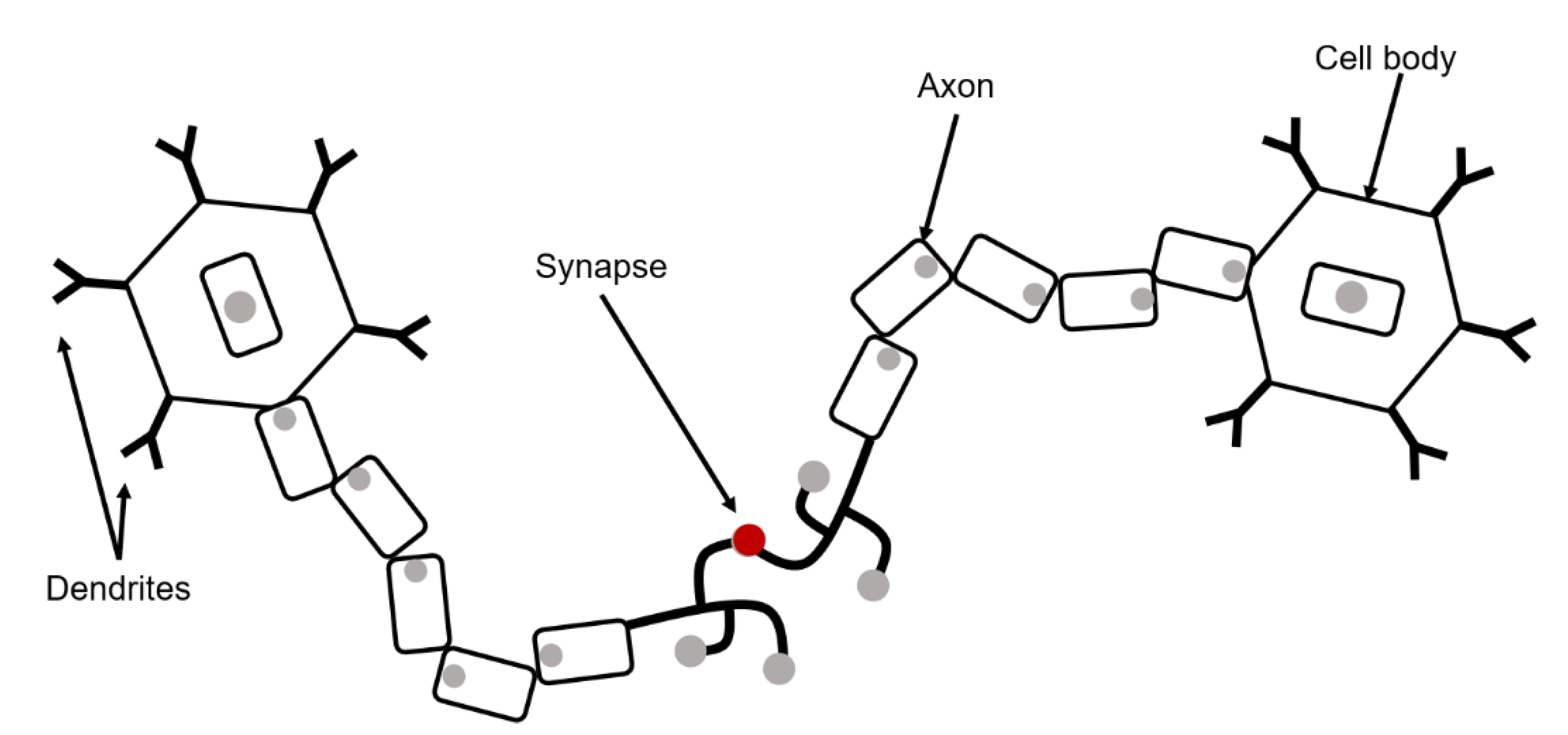
2. Artificial Neural Networks
2.1. The Activation Function of an Artificial Neural Network
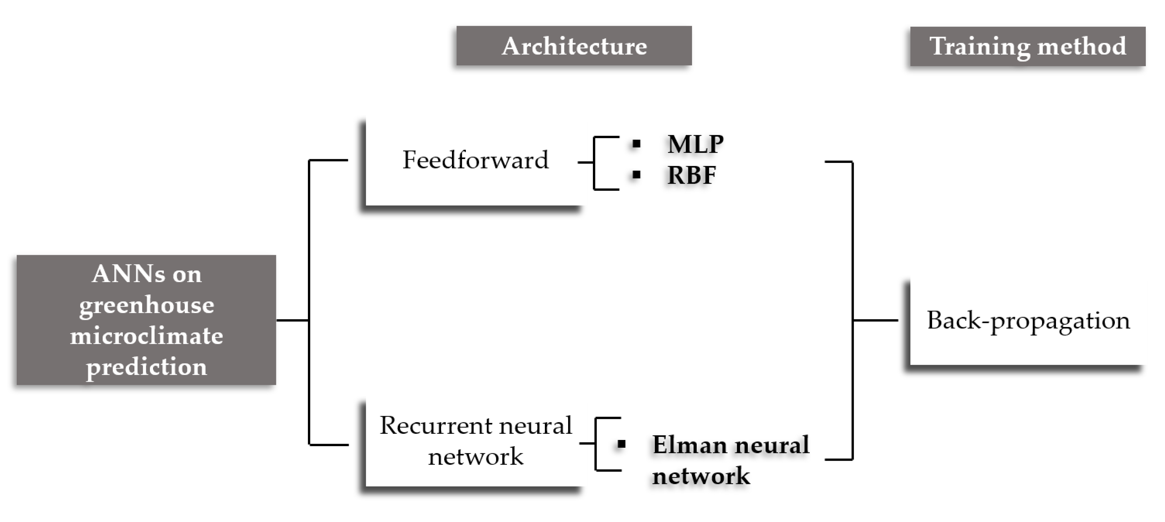
2.2. Types of Artificial Neural Network
- ▪
- Feedforward neural networks (FFNNs);
- ▪
- Recurrent neural networks (in discrete time) or differential (in continuous time);
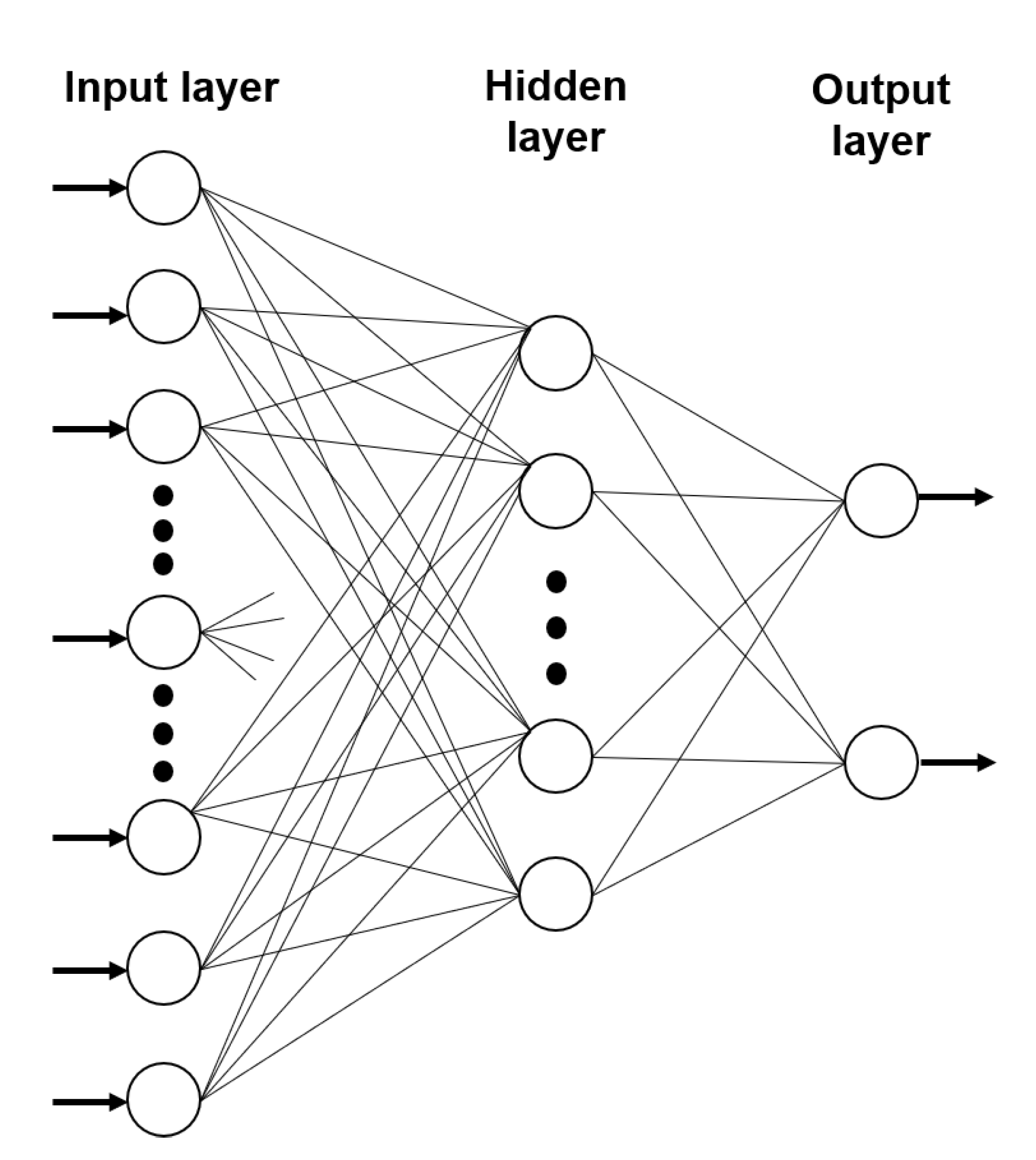
2.2.1. Feedforward Neural Networks
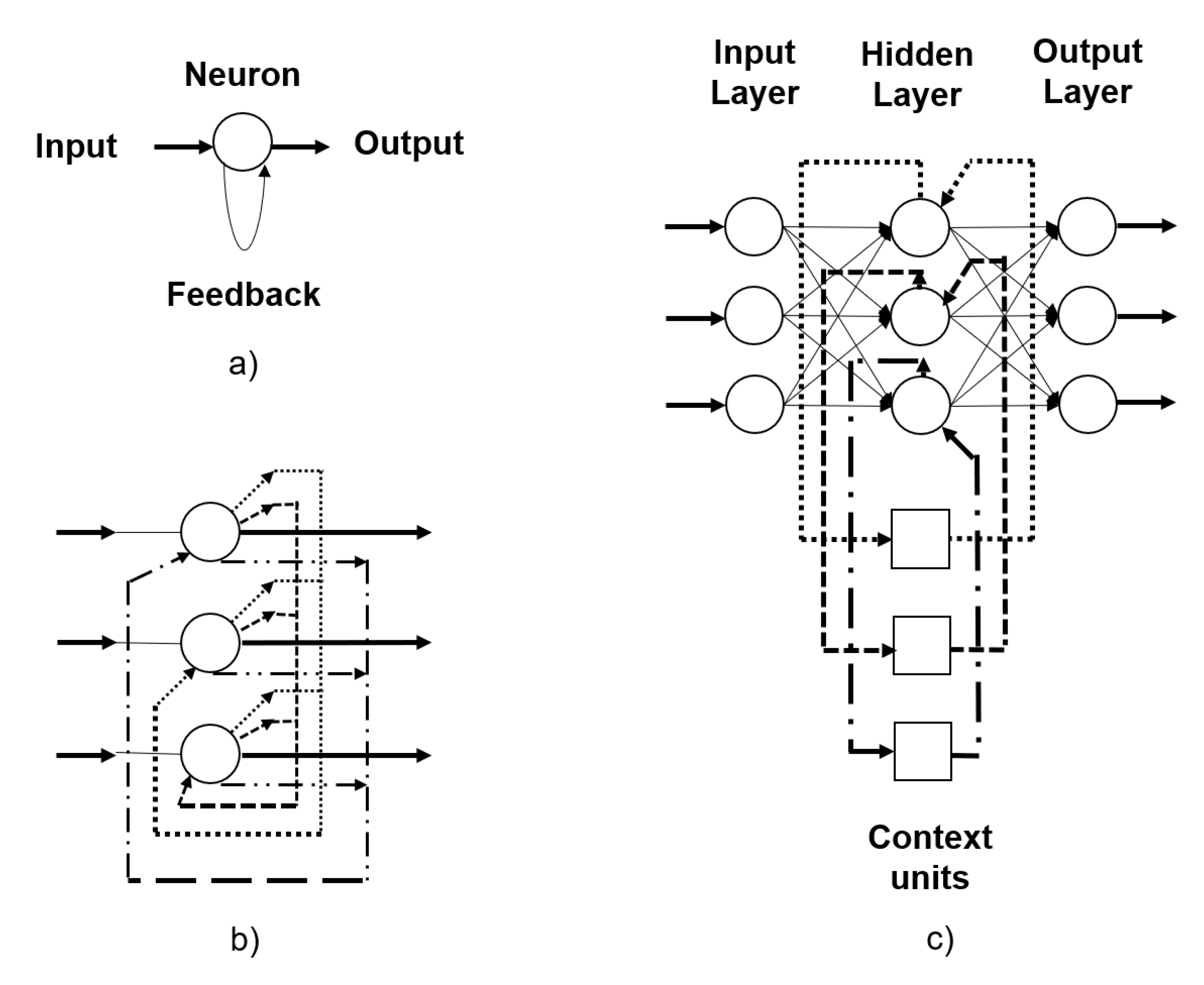
2.2.2. Recurrent Neural Networks
- ▪
- Hopfield network: each neuron is completely symmetrically connected with all other neurons in the network. If the connections are trained using Hebbian learning, then the Hopfield network can function as a solid memory and resistant to the alteration of the connection. Hebbian learning involves synapses between neurons and their strengthening when neurons on both sides of the synapse (input and output) have highly correlated outputs [87] as shown in Figure 5b. There is a guarantee in terms of convergence for this network [88].
- ▪
- Elman network: this is a horizontal network where a set of “context” neurons is added. In Figure 5c the context units are connected to the hidden network layer fixed with a weight. The subsequent fixed connections result in the context units always keeping a copy of the previous values of the hidden units, maintaining a state, which allows sequence prediction tasks [89].
- ▪
- Jordan network: these are very similar to Elman’s networks. However, context units feed on the output layer instead of the hidden layer.
2.3. Learning of Artificial Neural Networks
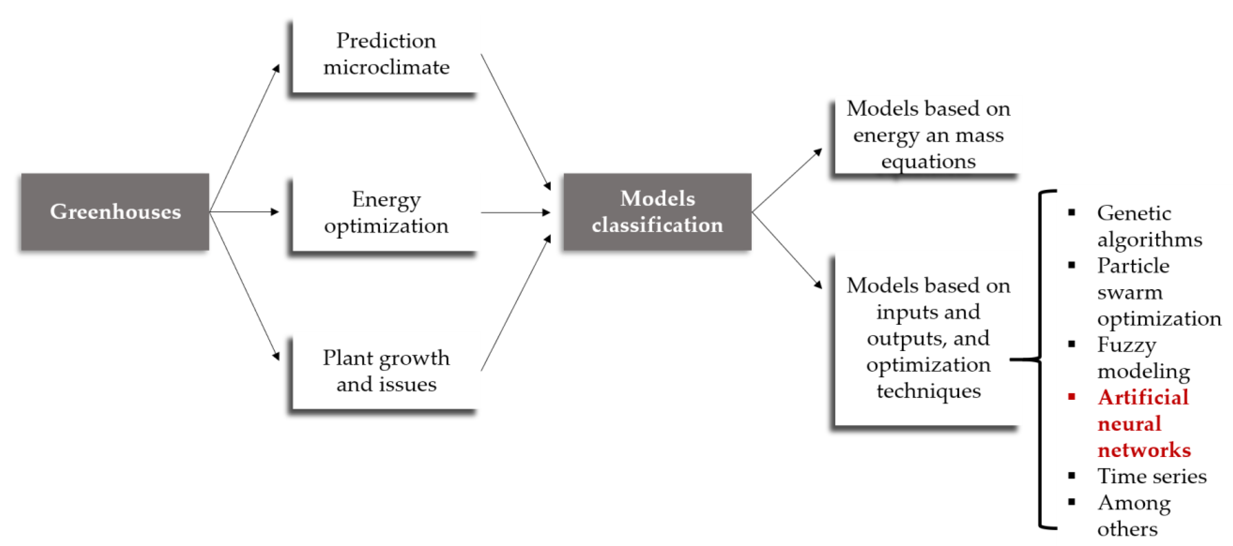
3. Application of Artificial Neural Networks for the Prediction of the Greenhouse Microclimate
3.1. Greenhouse Microclimate
3.2. Feedforward Neural Networks Models for Prediction of Microclimate in Greenhouse
3.3. Recurrent Neural Networks Models for Prediction of Microclimate in Greenhouses
3.4. Other Artificial Neural Networks Models for Prediction of Microclimate in Greenhouses
4. Artificial Neural Networks in Energy Optimization of Greenhouses
5. Other Applications of Artificial Neural Networks in Greenhouses
6. Perspectives: Greenhouse Artificial Neural Networks Application
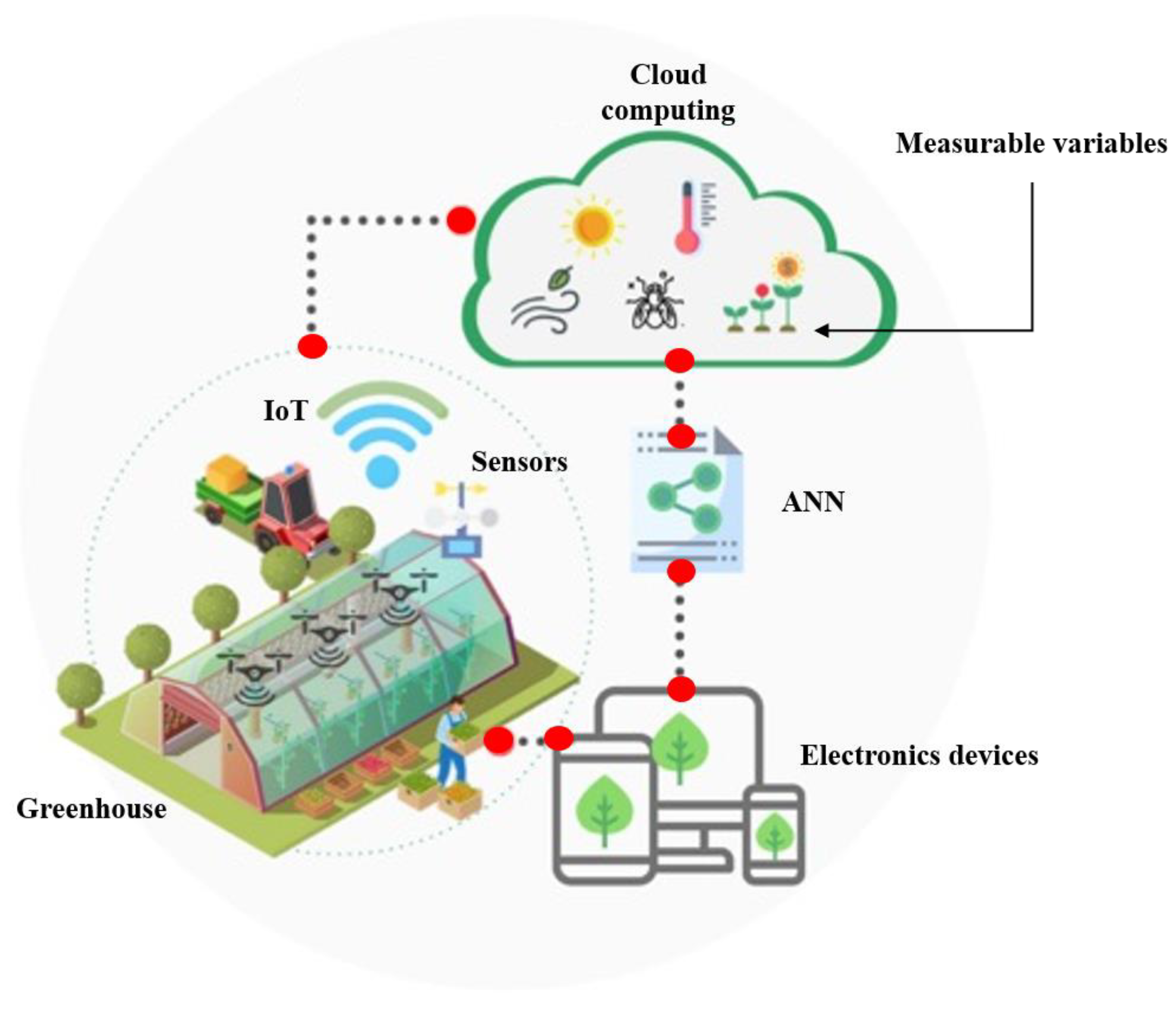
6.1. Agriculture 4.0 and the ANNs
6.1.1. Precision Agriculture and Internet of Things
6.1.2. Smart Agriculture
6.2. Artificial Neural Networks and Greenhouses
6.3. Classic Models versus ANNs
6.4. The Input Variables in the ANNs and in the Prediction of Greenhouse Microclimate
6.5. The Hidden Layer of ANNs and Their Importance in Prediction of Greenhouse Microclimate
6.6. Learning Algorithms in the ANNs
6.7. Database for ANNs and Prediction of Greenhouse Microclimate
6.8. Artificial Intelligence
6.9. Future of Deep Learning in Greenhouse Agriculture
6.10. Future of Hybrid ANNs in Greenhouse Agriculture
7. Guidelines for the Application of Neural Networks in Greenhouses
8. Conclusions
Author Contributions
Funding
Acknowledgments
Conflicts of Interest
References
- De Gelder, A.; Dieleman, J.A.; Bot, G.P.A.; Marcelis, L.F.M. An Overview of Climate and Crop Yield in Closed Greenhouses. J. Hortic. Sci. Biotechnol. 2012, 87, 193–202. [Google Scholar] [CrossRef]
- Gupta, M.K.; Chandra, P.; Samuel, D.V.K.; Singh, B.; Singh, A.; Garg, M.K. Modeling of Tomato Seedling Growth in Greenhouse. Agric. Res. 2012, 1, 362–369. [Google Scholar] [CrossRef]
- Iga, J.L. Modeling of the Climate for a Greenhouse in the North-East of México. IFAC Proc. Vol. 2008, 41, 9558–9563. [Google Scholar] [CrossRef] [Green Version]
- Van Straten, G.; Van Henten, E.J. Optimal Greenhouse Cultivation Control: Survey and Perspectives. IFAC Proc. Vol. 2010, 3. [Google Scholar] [CrossRef] [Green Version]
- Frausto, H.U.; Pieters, J.G. Modelling Greenhouse Temperature Using System Identification by Means of Neural Networks. Neurocomputing 2004, 56, 423–428. [Google Scholar] [CrossRef] [Green Version]
- Fitz-Rodríguez, E.; Kubota, C.; Giacomelli, G.A.; Tignor, M.E.; Wilson, S.B.; McMahon, M. Dynamic Modeling and Simulation of Greenhouse Environments under Several Scenarios: A Web-Based Application. Comput. Electron. Agric. 2010, 70, 105–116. [Google Scholar] [CrossRef]
- Azaza, M.; Echaieb, K.; Tadeo, F.; Fabrizio, E.; Iqbal, A.; Mami, A. Fuzzy Decoupling Control of Greenhouse Climate. Arab. J. Sci. Eng. 2015, 40, 2805–2812. [Google Scholar] [CrossRef]
- Ben Ali, R.; Bouadila, S.; Mami, A. Experimental Validation of the Dynamic Thermal Behavior of Two Types of Agricultural Greenhouses in the Mediterranean Context. Renew. Energy 2020, 147, 118–129. [Google Scholar] [CrossRef]
- Chalabi, Z.S.; Bailey, B.J.; Wilkinson, D.J. A Real-Time Optimal Control Algorithm for Greenhouse Heating. Comput. Electron. Agric. 1996, 15, 1–13. [Google Scholar] [CrossRef]
- Liang, M.H.; Chen, L.J.; He, Y.F.; Du, S.F. Greenhouse Temperature Predictive Control for Energy Saving Using Switch Actuators. IFAC PapersOnLine 2018, 51, 747–751. [Google Scholar] [CrossRef]
- Maher, A.; Kamel, E.; Enrico, F.; Atif, I.; Abdelkader, M. An Intelligent System for the Climate Control and Energy Savings in Agricultural Greenhouses. Energy Effic. 2016, 9, 1241–1255. [Google Scholar] [CrossRef]
- Nebbali, R.; Roy, J.C.; Boulard, T. Dynamic Simulation of the Distributed Radiative and Convective Climate within a Cropped Greenhouse. Renew. Energy 2012, 43, 111–129. [Google Scholar] [CrossRef]
- Su, Y.; Xu, L. Towards Discrete Time Model for Greenhouse Climate Control. Eng. Agric. Environ. Food 2017, 10, 157–170. [Google Scholar] [CrossRef]
- Fourati, F. Multiple Neural Control of a Greenhouse. Neurocomputing 2014, 139, 138–144. [Google Scholar] [CrossRef]
- Bennis, N.; Duplaix, J.; Enéa, G.; Haloua, M.; Youlal, H. Greenhouse Climate Modelling and Robust Control. Comput. Electron. Agric. 2008, 61, 96–107. [Google Scholar] [CrossRef]
- Coelho, J.P.; de Moura Oliveira, P.B.; Cunha, J.B. Greenhouse Air Temperature Predictive Control Using the Particle Swarm Optimisation Algorithm. Comput. Electron. Agric. 2005, 49, 330–344. [Google Scholar] [CrossRef] [Green Version]
- Montoya, A.P.; Guzmán, J.L.; Rodríguez, F.; Sánchez-Molina, J.A. A Hybrid-Controlled Approach for Maintaining Nocturnal Greenhouse Temperature: Simulation Study. Comput. Electron. Agric. 2016, 123, 116–124. [Google Scholar] [CrossRef]
- Hui, Z.; Lin-lin, Q.; Gang, W. Modeling and Simulation of Greenhouse Temperature Hybrid System Based on ARMAX Model. In Proceedings of the 2017 36th Chinese Control Conference, Dalian, China, 26–28 July 2017; IEEE: Piscatoway, IJ, USA, 2017; pp. 2237–2241. [Google Scholar] [CrossRef]
- Gerasimov, D.N.; Lyzlova, M.V. Adaptive Control of Microclimate in Greenhouses. J. Comput. Syst. Sci. Int. 2014, 53, 896–907. [Google Scholar] [CrossRef]
- Zabczyk, J. Mathematical Control Theory: An Introduction; Springer Science & Business Media: New York, NY, USA, 2009. [Google Scholar]
- Chen, L.; Du, S.; He, Y.; Liang, M.; Xu, D. Robust Model Predictive Control for Greenhouse Temperature Based on Particle Swarm Optimization. Inf. Process. Agric. 2018, 5, 329–338. [Google Scholar] [CrossRef]
- Rodríguez, C.; Guzman, J.L.; Rodríguez, F.; Berenguel, M.; Arahal, M.R. Diurnal Greenhouse Temperature Control with Predictive Control and Online Constrains Mapping. IFAC Proc. Vol. 2010, 1, 140–145. [Google Scholar] [CrossRef]
- Nielsen, B.; Madsen, H. Predictive Control of Air Temperature in Greenhouses. IFAC Proc. Vol. 1996, 29, 902–907. [Google Scholar] [CrossRef]
- Sigrimis, N.; Paraskevopoulos, P.N.; Arvanitis, K.G.; Rerras, N. Adaptive Temperature Control in Greenhouses Based on Multirate-Output Controllers. IFAC Proc. Vol. 1999, 32, 3760–3765. [Google Scholar] [CrossRef]
- Mohamed, S.; Hameed, I.A. A GA-Based Adaptive Neuro-Fuzzy Controller for Greenhouse Climate Control System. Alex. Eng. J. 2018, 57, 773–779. [Google Scholar] [CrossRef] [Green Version]
- Atia, D.M.; El-madany, H.T. Analysis and Design of Greenhouse Temperature Control Using Adaptive Neuro-Fuzzy Inference System. J. Electr. Syst. Inf. Technol. 2017, 4, 34–48. [Google Scholar] [CrossRef]
- Xu, D.; Du, S.; van Willigenburg, G. Adaptive Two Time-Scale Receding Horizon Optimal Control for Greenhouse Lettuce Cultivation. Comput. Electron. Agric. 2018, 146, 93–103. [Google Scholar] [CrossRef]
- Piñón, S.; Peña, M.; Soria, C.; Kuchen, B. Nonlinear Model Predictive Control via Feedback Linearization of a Greenhouse. IFAC Proc. Vol. 2000, 33, 191–196. [Google Scholar] [CrossRef]
- Pasgianos, G.D.; Arvanitis, K.G.; Polycarpou, P.; Sigrimis, N. A Nonlinear Feedback Technique for Greenhouse Environmental Control. Comput. Electron. Agric. 2003, 40, 153–177. [Google Scholar] [CrossRef]
- Ben Ali, R.; Bouadila, S.; Mami, A. Development of a Fuzzy Logic Controller Applied to an Agricultural Greenhouse Experimentally Validated. Appl. Therm. Eng. 2018, 141, 798–810. [Google Scholar] [CrossRef]
- Ramos-Fernández, J.C.; Balmat, J.F.; Márquez-Vera, M.A.; Lafont, F.; Pessel, N.; Espinoza-Quesada, E.S. Fuzzy Modeling Vapor Pressure Deficit to Monitoring Microclimate in Greenhouses. IFAC-PapersOnLine 2016, 49, 371–374. [Google Scholar] [CrossRef]
- Agmail, W.I.R.; Linker, R.; Arbel, A. Robust Control of Greenhouse Temperature and Humidity. IFAC Proc. 2009, 42, 138–143. [Google Scholar] [CrossRef]
- Linker, R.; Kacira, M.; Arbel, A. Robust Climate Control of a Greenhouse Equipped with Variable-Speed Fans and a Variable-Pressure Fogging System. Biosyst. Eng. 2011, 110, 153–167. [Google Scholar] [CrossRef]
- Moreno, J.C.; Berenguel, M.; Rodríguez, F.; Baños, A. Robust Control of Greenhouse Climate Exploiting Measurable Disturbances. IFAC Proc. 2002, 35, 271–276. [Google Scholar] [CrossRef] [Green Version]
- Xu, D.; Du, S.; van Willigenburg, G. Double Closed-Loop Optimal Control of Greenhouse Cultivation. Control Eng. Pract. 2019, 85, 90–99. [Google Scholar] [CrossRef]
- Xu, D.; Du, S.; van Willigenburg, L.G. Optimal Control of Chinese Solar Greenhouse Cultivation. Biosyst. Eng. 2018, 171, 205–219. [Google Scholar] [CrossRef]
- Van Ooteghem, R.J.C. Optimal Control Design for a Solar Greenhouse. IFAC Proc. Vol. 2010, 3. [Google Scholar] [CrossRef]
- Zeng, S.; Hu, H.; Xu, L.; Li, G. Nonlinear Adaptive PID Control for Greenhouse Environment Based on RBF Network. Sensors 2012, 12, 5328–5348. [Google Scholar] [CrossRef] [Green Version]
- Asa’d, O.; Ugursal, V.I.; Ben-Abdallah, N. Investigation of the Energetic Performance of an Attached Solar Greenhouse through Monitoring and Simulation. Energy Sustain. Dev. 2019, 53, 15–29. [Google Scholar] [CrossRef]
- Shahbazi, R.; Kouravand, S.; Hassan-Beygi, R. Analysis of Wind Turbine Usage in Greenhouses: Wind Resource Assessment, Distributed Generation of Electricity and Environmental Protection. Energy Sources Part A Recover. Util. Environ. Eff. 2019, 2019, 1–21. [Google Scholar] [CrossRef]
- Abdellatif, S.M.; El Ashmawy, N.M.; El-Bakhaswan, M.K.; Tarabye, H.H. Hybird, Solar and Biomass Energy System for Heating Greenhouse Sweet Coloured Pepper. Adv. Res. 2016, 2016, 1–21. [Google Scholar] [CrossRef]
- Bibbiani, C.; Fantozzi, F.; Gargari, C.; Campiotti, C.A.; Schettini, E.; Vox, G. Wood Biomass as Sustainable Energy for Greenhouses Heating in Italy. In Florence “Sustainability of Well-Being International Forum”. 2015: Food for Sustainability and not just food, FlorenceSWIF2015; Elsevier: Amsterdam, The Netherlands, 2016; pp. 637–645. [Google Scholar]
- Garzón, E.; Morales, L.; Ortiz-Rodríguez, I.M.; Sánchez-Soto, P.J. An Approach to the Heating Dynamics of Residues from Greenhouse-Crop Plant Biomass Originated by Tomatoes (Solanum Lycopersicum, L.). Environ. Sci. Pollut. Res. 2018, 25, 25880–25887. [Google Scholar] [CrossRef]
- Urbancl, D.; Trop, P.; Goričanec, D. Geothermal Heat Potential-the Source for Heating Greenhouses in Southestern Europe. Therm. Sci. 2016, 20, 1061–1071. [Google Scholar] [CrossRef]
- Aljubury, I.M.A.; Ridha, H.D. Enhancement of Evaporative Cooling System in a Greenhouse Using Geothermal Energy. Renew. Energy 2017, 111, 321–331. [Google Scholar] [CrossRef]
- Ozturk, H.H. Present Status and Future Prospects of Geothermal Energy Use for Greenhouse Heating in Turkey. Sci. Pap. B Hortic. 2017, 61, 441–450. [Google Scholar]
- Seginer, I.; van Beveren, P.J.M.; van Straten, G. Day-to-Night Heat Storage in Greenhouses: 3 Co-Generation of Heat and Electricity (CHP). Biosyst. Eng. 2018, 172, 1–18. [Google Scholar] [CrossRef]
- Compernolle, T.; Witters, N.; Van Passel, S.; Thewys, T. Analyzing a Self-Managed CHP System for Greenhouse Cultivation as a Profitable Way to Reduce CO2-Emissions. Energy 2011, 36, 1940–1947. [Google Scholar] [CrossRef]
- Vourdoubas, J. Overview of the Use of Sustainable Energies in Agricultural Greenhouses. J. Agric. Sci. 2016, 8, 36–43. [Google Scholar] [CrossRef] [Green Version]
- Mohammadi, B.; Ranjbar, F.; Ajabshirchi, Y. Exergoeconomic Analysis and Multi-Objective Optimization of a Semi-Solar Greenhouse with Experimental Validation. Appl. Therm. Eng. 2020, 164, 114563. [Google Scholar] [CrossRef]
- Ziapour, B.M.; Hashtroudi, A. Performance Study of an Enhanced Solar Greenhouse Combined with the Phase Change Material Using Genetic Algorithm Optimization Method. Appl. Therm. Eng. 2017, 110, 253–264. [Google Scholar] [CrossRef]
- Wang, J.; Li, S.; Guo, S.; Ma, C.; Wang, J.; Jin, S. Simulation and Optimization of Solar Greenhouses in Northern Jiangsu Province of China. Energy Build. 2014, 78, 143–152. [Google Scholar] [CrossRef]
- Zhang, X.; Lv, J.; Dawuda, M.M.; Xie, J.; Yu, J.; Gan, Y.; Zhang, J.; Tang, Z.; Li, J. Innovative Passive Heat-Storage Walls Improve Thermal Performance and Energy Efficiency in Chinese Solar Greenhouses for Non-Arable Lands. Sol. Energy 2019, 190, 561–575. [Google Scholar] [CrossRef]
- Mobtaker, H.G.; Ajabshirchi, Y.; Ranjbar, S.F.; Matloobi, M. Simulation of Thermal Performance of Solar Greenhouse in North-West of Iran: An Experimental Validation. Renew. Energy 2019, 135, 88–97. [Google Scholar] [CrossRef]
- Tong, G.; Christopher, D.M.; Li, B. Numerical Modelling of Temperature Variations in a Chinese Solar Greenhouse. Comput. Electron. Agric. 2009, 68, 129–139. [Google Scholar] [CrossRef]
- He, X.; Wang, J.; Guo, S.; Zhang, J.; Wei, B.; Sun, J.; Shu, S. Ventilation Optimization of Solar Greenhouse with Removable Back Walls Based on CFD. Comput. Electron. Agric. 2018, 149, 16–25. [Google Scholar] [CrossRef]
- Zhang, G.; Fu, Z.; Yang, M.; Liu, X.; Dong, Y.; Li, X. Nonlinear Simulation for Coupling Modeling of Air Humidity and Vent Opening in Chinese Solar Greenhouse Based on CFD. Comput. Electron. Agric. 2019, 162, 337–347. [Google Scholar] [CrossRef]
- Nicolosi, G.; Volpe, R.; Messineo, A. An Innovative Adaptive Control System to Regulate Microclimatic Conditions in a Greenhouse. Energies 2017, 10, 722. [Google Scholar] [CrossRef] [Green Version]
- Roy, R.; Furuhashi, T.; Chawdhry, P.K. Advances in Soft Computing: Engineering Design and Manufacturing; Springer Science & Business Media: New York, NY, USA, 2012. [Google Scholar]
- He, F.; Ma, C. Modeling Greenhouse Air Humidity by Means of Artificial Neural Network and Principal Component Analysis. Comput. Electron. Agric. 2010, 71, S19–S23. [Google Scholar] [CrossRef]
- Shanmuganathan, S. Artificial Neural Network Modelling: An Introduction. In Artificial Neural Network Modelling; Springer: New York, NY, USA, 2016; pp. 1–14. [Google Scholar]
- Hagan, M.T.; Demuth, H.B.; Beale, M.H. Neural Network Design: Campus Pub. Serv. Univ. Color. Bookst. 2002, 1284, 30–39. [Google Scholar]
- Akbari, M.; Asadi, P.; Givi, M.K.B.; Khodabandehlouie, G. Artificial Neural Network and Optimization. In Advances in Friction-Stir Welding and Processing; Elsevier: Waltham, UK, 2014; pp. 543–599. [Google Scholar] [CrossRef]
- Kalogirou, S.A. Artificial Neural Networks in Renewable Energy Systems Applications: A Review. Renew. Sustain. Energy Rev. 2000, 5, 373–401. [Google Scholar] [CrossRef]
- Deb, A.K. Introduction to Soft Computing Techniques: Artificial Neural Networks, Fuzzy Logic and Genetic Algorithms. Soft Comput. Text. Eng. 2011, 3–24. [Google Scholar] [CrossRef]
- Han, S.-H.; Kim, K.W.; Kim, S.; Youn, Y.C. Artificial Neural Network: Understanding the Basic Concepts without Mathematics. Dement. Neurocogn. Disord. 2018, 17, 83–89. [Google Scholar] [CrossRef]
- Profillidis, V.A.; Botzoris, G.N. Artificial Intelligence—Neural Network Methods. In Modeling of Transport Demand; Elsevier: Amsterdam, The Netherlands, 2019; pp. 353–382. [Google Scholar] [CrossRef]
- de B. Harrington, P. Sigmoid Transfer Functions in Backpropagation Neural Networks. Anal. Chem. 1993, 65, 2167–2168. [Google Scholar] [CrossRef]
- Sibi, P.; Jones, S.A.; Siddarth, P. Analysis of Different Activation Functions Using Back Propagation Neural Networks. J. Theor. Appl. Inf. Technol. 2013, 47, 1264–1268. [Google Scholar]
- Özkan, C.; Erbek, F.S. The Comparison of Activation Functions for Multispectral Landsat TM Image Classification. Photogramm. Eng. Remote Sens. 2003, 69, 1225–1234. [Google Scholar] [CrossRef]
- Zamanlooy, B.; Mirhassani, M. Efficient VLSI Implementation of Neural Networks with Hyperbolic Tangent Activation Function. IEEE Trans. Very Large Scale Integr. Syst. 2013, 22, 39–48. [Google Scholar] [CrossRef]
- Csáji, B.C. Approximation with Artificial Neural Networks. Fac. Sci. Etvs Lornd Univ. Hung. 2001, 24, 7. [Google Scholar]
- Dalton, J.; Deshmane, A. Artificial Neural Networks. IEEE Potentials 1991, 10, 33–36. [Google Scholar] [CrossRef]
- Wang, S.-C. Artificial Neural Network. In Interdisciplinary Computing in Java Programming; Springer US: Boston, MA, USA, 2003; pp. 81–100. [Google Scholar] [CrossRef]
- Namin, A.H.; Leboeuf, K.; Wu, H.; Ahmadi, M. Artificial Neural Networks Activation Function HDL Coder. In Proceedings of the 2009 IEEE International Conference on Electro/Information Technology, Windsor, ON, Canada, 7–9 June 2009; pp. 389–392. [Google Scholar] [CrossRef]
- Basterretxea, K.; Tarela, J.M.; Del Campo, I. Approximation of Sigmoid Function and the Derivative for Hardware Implementation of Artificial Neurons. IEE Proc. Circuits Devices Syst. 2004, 151, 18–24. [Google Scholar] [CrossRef]
- Han, X.; Hou, M. Neural Networks for Approximation of Real Functions with the Gaussian Functions. In Proceedings of the Third International Conference on Natural Computation, Haikou, China, 24–27 August 2007; pp. 601–605. [Google Scholar] [CrossRef]
- Kwon, S.J. Artificial Neural Networks. Artif. Neural Netw. 2011, 1–426. [Google Scholar] [CrossRef] [Green Version]
- Sajja, P.S.; Akerkar, R. Bio-Inspired Models for Semantic Web. In Swarm Intelligence and Bio-Inspired Computation; Elsevier: Amsterdam, The Netherlands, 2013; pp. 273–294. [Google Scholar]
- Suk, H., II. An Introduction to Neural Networks and Deep Learning, 1st ed.; Elsevier Inc.: Philadelphia, PA, USA, 2017. [Google Scholar] [CrossRef]
- Ben Nasr, M.; Chtourou, M. A Self-Organizing Map-Based Initialization for Hybrid Training of Feedforward Neural Networks. Appl. Soft Comput. 2011, 11, 4458–4464. [Google Scholar] [CrossRef]
- Sazlı, M.H. A Brief Review of Feed-Forward Neural Networks. Commun. Fac. Sci. Univ. Ank. Ser. A2-A3 2006, 50, 11–17. Available online: https://pdfs.semanticscholar.org/5a45/fb35ffad65c904da2edeef443dcf11219de7.pdf (accessed on 3 May 2020).
- Wythoff, B.J. Backpropagation Neural Networks: A Tutorial. Chemom. Intell. Lab. Syst. 1993, 18, 115–155. [Google Scholar] [CrossRef]
- Saikia, P.; Baruah, R.D.; Singh, S.K.; Chaudhuri, P.K. Artificial Neural Networks in the Domain of Reservoir Characterization: A Review from Shallow to Deep Models. Comput. Geosci. 2019, 2019, 104357. [Google Scholar] [CrossRef]
- Zupan, J. Basics of Artificial Neural Network. In Nature-inspired Methods in Chemometrics: Genetic Algorithms and Artificial Neural Networks, 1st ed.; Leardi, R., Ed.; Elsevier Science: New York, NY, USA, 2003; Volume 23, pp. 199–229. [Google Scholar]
- Poznyak, T.I.; Chairez Oria, I.; Poznyak, A.S. Background on Dynamic Neural Networks. In Ozonation and Biodegradation in Environmental Engineering; Elsevier: Amsterdam, The Netherlands, 2019; pp. 57–74. [Google Scholar] [CrossRef]
- Szandała, T. Comparison of Different Learning Algorithms for Pattern Recognition with Hopfield’s Neural Network. Procedia Comput. Sci. 2015, 71, 68–75. [Google Scholar] [CrossRef] [Green Version]
- Neapolitan, R.E.; Neapolitan, R.E. Neural Networks and Deep Learning. Artif. Intell. 2018, 389–411. [Google Scholar] [CrossRef]
- Şeker, S.; Ayaz, E.; Türkcan, E. Elman’s Recurrent Neural Network Applications to Condition Monitoring in Nuclear Power Plant and Rotating Machinery. Eng. Appl. Artif. Intell. 2003, 16, 647–656. [Google Scholar] [CrossRef]
- Yang, H.H.; Murata, N.; Amari, S.I. Statistical Inference: Learning in Artificial Neural Networks. Trends Cogn. Sci. 1998, 2, 4–10. [Google Scholar] [CrossRef]
- Guyon, I. Neural Networks and Applications Tutorial. Phys. Rep. 1991, 207, 215–259. [Google Scholar] [CrossRef]
- Suárez Gómez, S.L.; Santos Rodríguez, J.D.; Iglesias Rodríguez, F.J.; de Cos Juez, F.J. Analysis of the Temporal Structure Evolution of Physical Systems with the Self-Organising Tree Algorithm (SOTA): Application for Validating Neural Network Systems on Adaptive Optics Data before on-Sky Implementation. Entropy 2017, 19, 103. [Google Scholar] [CrossRef] [Green Version]
- Pakkanen, J.; Iivarinen, J.; Oja, E. The Evolving Tree—a Novel Self-Organizing Network for Data Analysis. Neural Process. Lett. 2004, 20, 199–211. [Google Scholar] [CrossRef]
- Milone, D.H.; Sáez, J.C.; Simón, G.; Rufiner, H.L. Self-Organizing Neural Tree Networks. In Proceedings of the 20th Annual International Conference of the IEEE Engineering in Medicine and Biology Society, Hong Kong, China, 1 November 1998; pp. 1348–1351. [Google Scholar] [CrossRef]
- Wen, W.X.; Jennings, A.; Liu, H. Learning a Neural Tree. In Proceedings International Joint Conference on Neural Networks; Citeseer: Berkeley, CA, USA, 1992. [Google Scholar]
- Seginer, I. Some Artificial Neural Network Applications to Greenhouse Environmental Control. Comput. Electron. Agric. 1997, 18, 167–186. [Google Scholar] [CrossRef]
- Bakker, J.C.; Bot, G.P.A.; Challa, H.; Van de Braak, N.J.; Sramek, F. Greenhouse Climate Control. An Integrated Approach. Biol. Plant. 1996, 38, 184. [Google Scholar]
- Bot, G.P.A. Greenhouse Climate: From Physical Processes to a Dynamic Model, Landbouwhogeschool te Wageningen. 1983. Available online: https://library.wur.nl/WebQuery/wurpubs/77514 (accessed on 3 May 2020).
- Hu, H.-G.; Xu, L.-H.; Wei, R.-H.; Zhu, B.-K. RBF Network Based Nonlinear Model Reference Adaptive PD Controller Design for Greenhouse Climate. Int. J. Adv. Comput. Technol 2011, 3, 357–366. [Google Scholar]
- Joudi, K.A.; Farhan, A.A. A Dynamic Model and an Experimental Study for the Internal Air and Soil Temperatures in an Innovative Greenhouse. Energy Convers. Manag. 2015, 91, 76–82. [Google Scholar] [CrossRef]
- Lopez, A.; Valera, D.L.; Molina-Aiz, F.D.; Pena, A. Sonic Anemometry to Evaluate Airflow Characteristics and Temperature Distribution in Empty Mediterranean Greenhouses Equipped with Pad–Fan and Fog Systems. Biosyst. Eng. 2012, 113, 334–350. [Google Scholar] [CrossRef]
- Jiang, Y.; Qin, L.; Qiu, Q.; Zheng, W.; Ma, G. Greenhouse Humidity System Modeling and Controlling Based on Mixed Logical Dynamical. In Proceedings of the 33rd Chinese Control Conference, Nanjing, China, 28–30 July 2014. pp. 4039–4043. [CrossRef]
- Yang, S.-H.; Lee, C.G.; Ashtiani-Araghi, A.; Kim, J.Y.; Rhee, J.Y. Development and Evaluation of Combustion-Type CO2 Enrichment System Connected to Heat Pump for Greenhouses. Eng. Agric. Environ. food 2014, 7, 28–33. [Google Scholar] [CrossRef]
- Umeda, H.; Ahn, D.-H.; Iwasaki, Y.; Matsuo, S.; Takeya, S. A Cooling and CO2 Enrichment System for Greenhouse Production Using CO2 Clathrate Hydrate. Eng. Agric. Environ. food 2015, 8, 307–312. [Google Scholar] [CrossRef]
- Dombaycı, Ö.A.; Gölcü, M. Daily Means Ambient Temperature Prediction Using Artificial Neural Network Method: A Case Study of Turkey. Renew. Energy 2009, 34, 1158–1161. [Google Scholar] [CrossRef]
- Chevalier, R.F.; Hoogenboom, G.; McClendon, R.W.; Paz, J.O. A Web-Based Fuzzy Expert System for Frost Warnings in Horticultural Crops. Environ. Model. Softw. 2012, 35, 84–91. [Google Scholar] [CrossRef]
- Martí, P.; Gasque, M.; GonzáLez-Altozano, P. An Artificial Neural Network Approach to the Estimation of Stem Water Potential from Frequency Domain Reflectometry Soil Moisture Measurements and Meteorological Data. Comput. Electron. Agric. 2013, 91, 75–86. [Google Scholar] [CrossRef]
- Li, N.; Wang, K.; Cheng, J. A Research on a Following Day Load Simulation Method Based on Weather Forecast Parameters. Energy Convers. Manag. 2015, 103, 691–704. [Google Scholar] [CrossRef]
- Cunha, J.B.; Couto, C.; Ruano, A.E.B. Real-Time Parameter Estimation of Dynamic Temperature Models for Greenhouse Environmental Control. Control Eng. Pract. 1997, 5, 1473–1481. [Google Scholar] [CrossRef]
- Pohlheim, H.; Heißner, A. Optimal Control of Greenhouse Climate Using a Short Time Climate Model and Evolutionary Algorithms. IFAC Proc. Vol. 1997, 30, 113–118. [Google Scholar] [CrossRef] [Green Version]
- Piñón, S.; Camacho, E.F.; Kuchen, B.; Peña, M. Constrained Predictive Control of a Greenhouse. Comput. Electron. Agric. 2005, 49, 317–329. [Google Scholar] [CrossRef]
- Ferreira, P.M.; Faria, E.A.; Ruano, A.E. Neural Network Models in Greenhouse Air Temperature Prediction. Neurocomputing 2002, 43, 51–75. [Google Scholar] [CrossRef] [Green Version]
- Márquez-Vera, M.A.; Ramos-Fernández, J.C.; Cerecero-Natale, L.F.; Lafont, F.; Balmat, J.-F.; Esparza-Villanueva, J.I. Temperature Control in a MISO Greenhouse by Inverting Its Fuzzy Model. Comput. Electron. Agric. 2016, 124, 168–174. [Google Scholar] [CrossRef]
- Lafont, F.; Balmat, J.-F. Fuzzy Logic to the Identification and the Command of the Multidimensional Systems. Int. J. Comput. Cogn. 2004, 2, 21–47. [Google Scholar]
- Lafont, F.; Balmat, J.-F. Optimized Fuzzy Control of a Greenhouse. Fuzzy Sets Syst. 2002, 128, 47–59. [Google Scholar] [CrossRef]
- Bennis, N.; Duplaix, J.; Enea, G.; Haloua, M.; Youlal, H. An Advanced Control of Greenhouse Climate. In Proceedings of the 33rd International Symposium Actual Tasks Agricultural Engineering, Croatia, Yugoslavia, 21–25 February 2005; pp. 265–277. [Google Scholar]
- Arvanitis, K.G.; Paraskevopoulos, P.N.; Vernardos, A.A. Multirate Adaptive Temperature Control of Greenhouses. Comput. Electron. Agric. 2000, 26, 303–320. [Google Scholar] [CrossRef]
- Revathi, S.; Sivakumaran, N. Fuzzy Based Temperature Control of Greenhouse. IFAC-PapersOnLine 2016, 49, 549–554. [Google Scholar] [CrossRef]
- Singh, V.K.; Tiwari, K.N. Prediction of Greenhouse Micro-Climate Using Artificial Neural Network. Appl. Ecol. Environ. Res. 2017, 15, 767–778. [Google Scholar] [CrossRef]
- González Pérez, I.; Calderón Godoy, A.J. Neural Networks-Based Models for Greenhouse Climate Control. Proceeding of En Actas de las XXXIX Jornadas de Automática, Badajoz, Spain, 5–7 September 2018; Available online: http://hdl.handle.net/10662/8744 (accessed on 3 May 2020).
- He, F.; Ma, C.; Zhang, J.; Chen, Y. Greenhouse Air Temperature and Humidity Prediction Based on Improved BP Neural Network and Genetic Algorithm. In International Symposium on Neural Networks; Springer: New York, NY, USA, 2007; pp. 973–980. [Google Scholar]
- da Silva, I.N.; Spatti, D.H.; Flauzino, R.A.; Liboni, L.H.B.; dos Reis Alves, S.F. Artificial Neural Network Architectures and Training Processes. In Artificial Neural Networks; Springer: New York, NY, USA, 2017; pp. 21–28. [Google Scholar]
- Dariouchy, A.; Aassif, E.; Lekouch, K.; Bouirden, L.; Maze, G. Prediction of the Intern Parameters Tomato Greenhouse in a Semi-Arid Area Using a Time-Series Model of Artificial Neural Networks. Measurement 2009, 42, 456–463. [Google Scholar] [CrossRef]
- Taki, M.; Ajabshirchi, Y.; Ranjbar, S.F.; Matloobi, M. Application of Neural Networks and Multiple Regression Models in Greenhouse Climate Estimation. Agric. Eng. Int. CIGR J. 2016, 18, 29–43. [Google Scholar]
- Seginer, I.; Boulard, T.; Bailey, B.J. Neural Network Models of the Greenhouse Climate. J. Agric. Eng. Res. 1994, 59, 203. [Google Scholar] [CrossRef]
- Laribi, I.; Homri, H.; Mhiri, R. Modeling of a Greenhouse Temperature: Comparison between Multimodel and Neural Approaches. In Proceedings of the 2006 IEEE International Symposium on Industrial Electronics, Montreal, QC, Canada, 9–13 July 2006; pp. 399–404. [Google Scholar] [CrossRef]
- Bussab, M.A.; Bernardo, J.I.; Hirakawa, A.R. Greenhouse Modeling Using Neural Networks. In Proceedings of the 6th WSEAS International Conference on Artificial Intelligence, Knowledge Engineering and Data Bases, Corfu Island, Greece, 16–19 February 2007; pp. 131–135. [Google Scholar]
- Salazar, R.; López, I.; Rojano, A. A Neural Network Model to Predict Temperature and Relative Humidity in a Greenhouse. In Proceedings of the International Symposium on High Technology for Greenhouse System Management: Greensys2007, Naples, Italy, 4–6 October 2007; pp. 539–546. [Google Scholar] [CrossRef]
- Alipour, M.; Loghavi, M. Development and Evaluation of a Comprehensive Greenhouse Climate Control System Using Artificial Neural Network. Univers. J. Control Autom. 2013, 1, 10–14. [Google Scholar]
- Outanoute, M.; Lachhab, A.; Selmani, A.; Oubehar, H.; Guerbaoui, M. Neural Network Based Models for Estimating the Temperature and Humidity under Greenhouse. Int. J. Multi Discip. Sci. 2016, 3, 26–33. [Google Scholar]
- Taki, M.; Abdanan Mehdizadeh, S.; Rohani, A.; Rahnama, M.; Rahmati-Joneidabad, M. Applied Machine Learning in Greenhouse Simulation; New Application and Analysis. Inf. Process. Agric. 2018, 5, 253–268. [Google Scholar] [CrossRef]
- Pham, D.T.; Liu, X. Artificial Neural Networks. In Neural Networks for Identification, Prediction and Control; Springer: New York, NY, USA, 1995; pp. 1–23. [Google Scholar]
- Fourati, F.; Chtourou, M. A Greenhouse Control with Feed-Forward and Recurrent Neural Networks. Simul. Model. Pract. Theory 2007, 15, 1016–1028. [Google Scholar] [CrossRef]
- Fourati, F.; Chtourou, M. A Greenhouse Neural Control Using Generalized and Specialized Learning. Int. J. Innov. Comput. Inf. Control 2011, 7, 5813–5824. [Google Scholar]
- Hongkang, W.; Li, L.; Yong, W.; Fanjia, M.; Haihua, W.; Sigrimis, N.A. Recurrent Neural Network Model for Prediction of Microclimate in Solar Greenhouse. IFAC PapersOnLine 2018, 51, 790–795. [Google Scholar] [CrossRef]
- Dahmani, K.; Elleuch, K.; Fourati, F.; Toumi, A. Adaptive Neural Control of a Greenhouse. 19th Int. Conf. Sci. Tech. Autom. Control Comput. Eng. STA 2019 2019, 2019, 59–63. [Google Scholar] [CrossRef]
- Salah, L.B.; Fourati, F. Systems Modeling Using Deep Elman Neural Network. Eng. Technol. Appl. Sci. Res. 2019, 9, 3881–3886. [Google Scholar]
- Rodríguez, F.; Arahal, M.R.; Berenguel, M. Application of Artificial Neural Networks for Greenhouse Climate Modelling. In Proceedings of the 1999 European Control Conference, Karlsruhe, Germany, 31 August –3 September 1999; pp. 2096–2101. [Google Scholar] [CrossRef]
- Manonmani, A.; Thyagarajan, T.; Elango, M.; Sutha, S. Modelling and Control of Greenhouse System Using Neural Networks. Trans. Inst. Meas. Control 2018, 40, 918–929. [Google Scholar] [CrossRef]
- Lu, T.; Viljanen, M. Prediction of Indoor Temperature and Relative Humidity Using Neural Network Models: Model Comparison. Neural Comput. Appl. 2009, 18, 345–357. [Google Scholar] [CrossRef]
- Zhang, X.Y. A Novel Greenhouse Control System Based on Fuzzy Neural Network. Appl. Mech. Mater. 2014, 668–669, 415–418. [Google Scholar] [CrossRef]
- Patil, S.L.; Tantau, H.J.; Salokhe, V.M. Modelling of Tropical Greenhouse Temperature by Auto Regressive and Neural Network Models. Biosyst. Eng. 2008, 99, 423–431. [Google Scholar] [CrossRef]
- Ghani, S.; Bakochristou, F.; ElBialy, E.M.A.A.; Gamaledin, S.M.A.; Rashwan, M.M.; Abdelhalim, A.M.; Ismail, S.M. Design Challenges of Agricultural Greenhouses in Hot and Arid Environments–A Review. Eng. Agric. Environ. Food 2019, 12, 48–70. [Google Scholar] [CrossRef]
- Bailey, B.J.; Seginer, I. Optimum Control of Greenhouse Heating. Eng. Econ. Asp. Energy Sav. Prot. Cultiv. 1988, 245, 512–518. [Google Scholar] [CrossRef]
- Nayak, S.; Tiwari, G.N. Energy and Exergy Analysis of Photovoltaic/Thermal Integrated with a Solar Greenhouse. Energy Build. 2008, 40, 2015–2021. [Google Scholar] [CrossRef]
- Ntinas, G.K.; Fragos, V.P.; Nikita-Martzopoulou, C. Thermal Analysis of a Hybrid Solar Energy Saving System inside a Greenhouse. Energy Convers. Manag. 2014, 81, 428–439. [Google Scholar] [CrossRef]
- Ahamed, M.S.; Guo, H.; Tanino, K. A Quasi-Steady State Model for Predicting the Heating Requirements of Conventional Greenhouses in Cold Regions. Inf. Process. Agric. 2018, 5, 33–46. [Google Scholar] [CrossRef]
- Chen, J.; Xu, F.; Tan, D.; Shen, Z.; Zhang, L.; Ai, Q. A Control Method for Agricultural Greenhouses Heating Based on Computational Fluid Dynamics and Energy Prediction Model. Appl. Energy 2015, 141, 106–118. [Google Scholar] [CrossRef]
- Chen, J.; Chen, J.; Yang, J.; Xu, F.; Shen, Z. Prediction on Energy Consumption of Semi-Closed Greenhouses Based on Self-Accelerating PSO-GA. Trans. Chinese Soc. Agric. Eng. 2015, 31, 186–193. [Google Scholar]
- Trejo-Perea, M.; Herrera-Ruiz, G.; Rios-Moreno, J.; Miranda, R.C.; Rivas-Araiza, E. Greenhouse Energy Consumption Prediction Using Neural Networks Models. Int. J. Agric. Biol. 2009, 11, 1–6. [Google Scholar]
- Pérez-Alonso, J.; Pérez-García, M.; Pasamontes-Romera, M.; Callejón-Ferre, A.J. Performance Analysis and Neural Modelling of a Greenhouse Integrated Photovoltaic System. Renew. Sustain. Energy Rev. 2012, 16, 4675–4685. [Google Scholar] [CrossRef]
- Taki, M.; Haddad, M. A Novel Method with Multilayer Feed-Forward Neural Network for Modeling Output Yield in Agriculture. Int. J. Mod. Agric. 2012, 1, 13–23. [Google Scholar]
- Tantau, H.-J. Energy Saving Potential of Greenhouse Climate Control. Math. Comput. Simul. 1998, 48, 93–101. [Google Scholar] [CrossRef]
- Ito, K.; Hattori, K. Numerical Prediction of Thermal Environment and Energy Consumption in Tunnel-Type Greenhouse with Supplementary Air-Mixing and Heating Device. Indoor Built Environ. 2012, 21, 292–303. [Google Scholar] [CrossRef]
- Bailey, B.J. Control Strategies to Enhance the Performance of Greenhouse Thermal Screens. J. Agric. Eng. Res. 1988, 40, 187–198. [Google Scholar] [CrossRef]
- Tantau, H.-J.; Meyer, J.; Schmidt, U.; Bessler, B. Low Energy Greenhouse-a System Approach. In Proceedings of the International Symposium on High Technology for Greenhouse Systems: GreenSys2009, Québec City, QC, Canada, 14–19 June 2009; ISHS Acta Horticulturae: Leuven, Belgium, 2011; pp. 75–84. [Google Scholar] [CrossRef]
- Linker, R.; Seginer, I.; Gutman, P.O. Optimal CO2 Control in a Greenhouse Modeled with Neural Networks. Comput. Electron. Agric. 1998, 19, 289–310. [Google Scholar] [CrossRef]
- Moon, T.W.; Jung, D.H.; Chang, S.H.; Son, J.E. Estimation of Greenhouse CO2 Concentration via an Artificial Neural Network That Uses Environmental Factors. Hortic. Environ. Biotechnol. 2018, 59, 45–50. [Google Scholar] [CrossRef]
- Ehret, D.L.; Hill, B.D.; Helmer, T.; Edwards, D.R. Neural Network Modeling of Greenhouse Tomato Yield, Growth and Water Use from Automated Crop Monitoring Data. Comput. Electron. Agric. 2011, 79, 82–89. [Google Scholar] [CrossRef]
- Juan, Z.; Jie, C.; Shanshan, W.; Lingxun, D. Modeling of the Growing Process of Tomato Based on Modified Elman Network and FGA. In Proceedings of the 2007 IEEE International Conference on Control and Automation, Guangzhou, China, 30 May–1 June 2007; pp. 2377–2380. [Google Scholar] [CrossRef]
- Xanthopoulos, G.T.; Athanasiou, A.A.; Lentzou, D.I.; Boudouvis, A.G.; Lambrinos, G.P. Modelling of Transpiration Rate of Grape Tomatoes. Semi-Empirical and Analytical Approach. Biosyst. Eng. 2014, 124, 16–23. [Google Scholar] [CrossRef]
- Wang, H.; Sánchez-Molina, J.A.; Li, M.; Berenguel, M.; Yang, X.T.; Bienvenido, J.F. Leaf Area Index Estimation for a Greenhouse Transpiration Model Using External Climate Conditions Based on Genetics Algorithms, Back-Propagation Neural Networks and Nonlinear Autoregressive Exogenous Models. Agric. Water Manag. 2017, 183, 107–115. [Google Scholar] [CrossRef]
- Cañete, E.; Chen, J.; Luque, R.M.; Rubio, B. NeuralSens: A Neural Network Based Framework to Allow Dynamic Adaptation in Wireless Sensor and Actor Networks. J. Netw. Comput. Appl. 2012, 35, 382–393. [Google Scholar] [CrossRef]
- Chi, T.; Chen, M.; Gao, Q. Implementation and Study of a Greenhouse Environment Surveillance System Based on Wireless Sensor Network. In Proceedings of the 2008 International Conference on Embedded Software and Systems Symposia, Sichuan, China, 29–31 July 2008; pp. 287–291. [Google Scholar] [CrossRef]
- Bai, X.; Wang, Z.; Zou, L.; Alsaadi, F.E. Collaborative Fusion Estimation over Wireless Sensor Networks for Monitoring CO2 Concentration in a Greenhouse. Inf. Fusion 2018, 42, 119–126. [Google Scholar] [CrossRef]
- Zhang, R.B.; Wang, L.H.; Huang, X.L.; Guo, J.J. Design of Greenhouse Wireless Sensor Network Control System Based on Fuzzy Neural Network. In Key Engineering Materials; Trans Tech Publ: Zurich, Switzerland, 2011; pp. 318–321. [Google Scholar]
- Ting, L.; Man, Z.; Yuhan, J.; Sha, S.; Yiqiong, J.; Minzan, L. Management of CO2 in a Tomato Greenhouse Using WSN and BPNN Techniques. Int. J. Agric. Biol. Eng. 2015, 8, 43–51. [Google Scholar]
- Zambon, I.; Cecchini, M.; Egidi, G.; Saporito, M.G.; Colantoni, A. Revolution 4.0: Industry vs. Agriculture in a Future Development for SMEs. Processes 2019, 7, 36. [Google Scholar] [CrossRef] [Green Version]
- Monteleone, S.; de Moraes, E.A.; Maia, R.F. Analysis of the Variables That Affect the Intention to Adopt Precision Agriculture for Smart Water Management in Agriculture 4.0 Context. In Proceedings of the 2019 Global IoT Summit (GIoTS), Aarhus, Denmark, 17–21 June 2019; pp. 1–6. [Google Scholar] [CrossRef]
- Association, E.A.M. Digital Farming: What Does It Really Mean. Position Pap. CEMA 2017. Available online: https://www.cema-agri.org/position-papers/254-digital-farming-what-does-it-really-mean (accessed on 3 May 2020).
- Balafoutis, A.T.; Beck, B.; Fountas, S.; Tsiropoulos, Z.; Vangeyte, J.; van der Wal, T.; Soto-Embodas, I.; Gómez-Barbero, M.; Pedersen, S.M. Smart Farming Technologies–Description, Taxonomy and Economic Impact. In Precision Agriculture: Technology and Economic Perspectives; Springer: New York, NY, USA, 2017; pp. 21–77. [Google Scholar]
- Saiz-Rubio, V.; Rovira-Más, F. From Smart Farming towards Agriculture 5.0: A Review on Crop Data Management. Agronomy 2020, 10, 207. [Google Scholar] [CrossRef] [Green Version]
- Lezoche, M.; Hernandez, J.; del Mar Alemany Diaz, M.; Panetto, H.; Kacprzyk, J. Agri-Food 4.0: A Survey of the Supply Chains and Technologies for the Future Agriculture. Comput. Ind. 2020, 116, 1–15. [Google Scholar] [CrossRef]
- Davis, G.; Casady, W.W.; Massey, R.E. Precision Agriculture: An Introduction. Ext. Publ. 1998. Available online: http://hdl.handle.net/10355/9432 (accessed on 3 May 2020).
- Pedersen, S.M.; Lind, K.M. Precision Agriculture–from Mapping to Site-Specific Application. In Precision Agriculture: Technology and Economic Perspectives; Springer: New York, NY, USA, 2017; pp. 1–20. [Google Scholar]
- Stafford, J.V. Implementing Precision Agriculture in the 21st Century. J. Agric. Eng. Res. 2000, 76, 267–275. [Google Scholar] [CrossRef] [Green Version]
- Pucheta, J.; Patiño, D.; Fullana, R.; Schugurensky, C.; Kuchen, B.C. Neurodynamic Programming-Based Optimal Control for Crop Growth in Precision Agriculture. In Proceedings of the 16th IFAC World Congress, Prague, Czech Republic, 4–8 July 2005; Available online: www.nt.ntnu.no/users/skoge/prost/proceedings/ifac2005/Papers/Paper5047.html (accessed on 3 May 2020).
- Mat, I.; Kassim, M.R.M.; Harun, A.N. Precision Irrigation Performance Measurement Using Wireless Sensor Network. In Proceedings of the 2014 Sixth International Conference on Ubiquitous and Future Networks, Shanghai, China, 8–11 July 2014; pp. 154–157. [Google Scholar] [CrossRef]
- Kassim, M.R.M.; Mat, I.; Harun, A.N. Wireless Sensor Network in Precision Agriculture Application. In Proceedings of the 2014 International Conference on Computer, Information and Telecommunication Systems, Jeju, Korea, 7–9 July 2014; pp. 1–5. [Google Scholar] [CrossRef]
- Dan, L.; Jianmei, S.; Yang, Y.; Jianqiu, X. Precise Agricultural Greenhouses Based on the IoT and Fuzzy Control. In Proceedings of the 2016 International Conference on Intelligent Transportation, Big Data & Smart City, Changsha, China, 17–18 December 2016; pp. 580–583. [Google Scholar] [CrossRef]
- Hamouda, Y.E.M.; Elhabil, B.H.Y. Precision Agriculture for Greenhouses Using a Wireless Sensor Network. In Proceedings of the 2017 Palestinian International Conference on Information and Communication Technology, Gaza City, Palestinian Authority, 8–9 May 2017; pp. 78–83. [Google Scholar] [CrossRef]
- Wolfert, S.; Goense, D.; Sørensen, C.A.G. A Future Internet Collaboration Platform for Safe and Healthy Food from Farm to Fork. In Proceedings of the 2014 Annual SRII Global Conference, San Jose, CA, USA, 23–25 April 2014; pp. 266–273. [Google Scholar] [CrossRef]
- Boursianis, A.D.; Papadopoulou, M.S.; Diamantoulakis, P.; Liopa-Tsakalidi, A.; Barouchas, P.; Salahas, G.; Karagiannidis, G.; Wan, S.; Goudos, S.K. Internet of Things (IoT) and Agricultural Unmanned Aerial Vehicles (UAVs) in Smart Farming: A Comprehensive Review. Internet Things 2020, 2020, 100187. [Google Scholar] [CrossRef]
- Villa-Henriksen, A.; Edwards, G.T.C.; Pesonen, L.A.; Green, O.; Sørensen, C.A.G. Internet of Things in Arable Farming: Implementation, Applications, Challenges and Potential. Biosyst. Eng. 2020, 191, 60–84. [Google Scholar] [CrossRef]
- Ullah, M.W.; Mortuza, M.G.; Kabir, M.H.; Ahmed, Z.U.; Supta, S.K.D.; Das, P.; Hossain, S.M.D. Internet of Things Based Smart Greenhouse: Remote Monitoring and Automatic Control. DEStech Trans. Environ. Energy Earth Sci. 2018. [Google Scholar] [CrossRef]
- Kitpo, N.; Kugai, Y.; Inoue, M.; Yokemura, T.; Satomura, S. Internet of Things for Greenhouse Monitoring System Using Deep Learning and Bot Notification Services. In Proceedings of the 2019 IEEE International Conference on Consumer Electronics, Las Vegas, NV, USA, 11–13 January 2019; pp. 1–4. [Google Scholar] [CrossRef]
- Tervonen, J. Experiment of the Quality Control of Vegetable Storage Based on the Internet-of-Things. Procedia Comput. Sci. 2018, 130, 440–447. [Google Scholar] [CrossRef]
- Wang, J.; Chen, M.; Zhou, J.; Li, P. Data Communication Mechanism for Greenhouse Environment Monitoring and Control: An Agent-Based IoT System. Inf. Process. Agric. 2019, in press. [Google Scholar] [CrossRef]
- Sinha, A.; Shrivastava, G.; Kumar, P. Architecting User-Centric Internet of Things for Smart Agriculture. Sustain. Comput. Inform. Syst. 2019, 23, 88–102. [Google Scholar] [CrossRef]
- Chiregi, M.; Navimipour, N.J. Cloud Computing and Trust Evaluation: A Systematic Literature Review of the State-of-the-Art Mechanisms. J. Electr. Syst. Inf. Technol. 2018, 5, 608–622. [Google Scholar] [CrossRef]
- Hasan, M.; Goraya, M.S. Fault Tolerance in Cloud Computing Environment: A Systematic Survey. Comput. Ind. 2018, 99, 156–172. [Google Scholar] [CrossRef]
- Aytekin, A.; AYAZ, A.; TÜMİNÇİN, F. Intelligent and Natural Agriculture with Industry 4.0. Bartın Orman Fakültesi Derg. 2019, 21, 938–944. [Google Scholar]
- Li, Z.; Wang, J.; Higgs, R.; Zhou, L.; Yuan, W. Design of an Intelligent Management System for Agricultural Greenhouses Based on the Internet of Things. In Proceedings of the 2017 IEEE International Conference on Computational Science and Engineering (CSE) and IEEE International Conference on Embedded and Ubiquitous Computing, Guangzhou, China, 21–24 July 2017; pp. 154–160. [Google Scholar] [CrossRef]
- Wu, X.; Zhu, X.; Wu, G.-Q.; Ding, W. Data Mining with Big Data. Ieee Transactions on Knowledge and Data Engineering 26, 1, 97--107. Google Sch. Digit. Libr. 2014, 26, 97–107. [Google Scholar] [CrossRef]
- Sharief, M.A.; Chowdhury, A. Thermal Computational Analysis of Micromclimates for Optimal Crop Production in Controlled Atmosphere. Energy Procedia 2019, 160, 783–790. [Google Scholar] [CrossRef]
- Yahya, N. Agricultural 4.0: Its Implementation toward Future Sustainability. In Green Urea; Springer: New York, NY, USA, 2018; pp. 125–145. [Google Scholar]
- Li, N.; Xiao, Y.; Shen, L.; Xu, Z.; Li, B.; Yin, C. Smart Agriculture with an Automated IoT-Based Greenhouse System for Local Communities. Adv. Internet Things 2019, 09, 15–31. [Google Scholar] [CrossRef] [Green Version]
- Jolliet, O. HORTITRANS, a Model for Predicting and Optimizing Humidity and Transpiration in Greenhouses. J. Agric. Eng. Res. 1994, 57, 23–37. [Google Scholar] [CrossRef]
- Kothari, S.; Panwar, N.L. Steady State Thermal Model for Predicting Micro-Climate inside the Greenhouse. J. Inst. Eng. (India) Agric. Eng. 2007, 88, 52–55. [Google Scholar]
- Mohammadi, B.; Ranjbar, S.F.; Ajabshirchi, Y. Application of Dynamic Model to Predict Some inside Environment Variables in a Semi-Solar Greenhouse. Inf. Process. Agric. 2018, 5, 279–288. [Google Scholar] [CrossRef]
- Hong, T.; Lee, S.H. Integrating Physics-Based Models with Sensor Data: An Inverse Modeling Approach. Build. Environ. 2019, 154, 23–31. [Google Scholar] [CrossRef] [Green Version]
- Van Straten, G.; van Willigenburg, G.; van Henten, E.; van Ooteghem, R. Optimal Control of Greenhouse Cultivation; CRC Press: Boca Raton, FL, USA, 2010. [Google Scholar]
- Llera, J.R.; Deb, K.; Runkle, E.; Xu, L.; Goodman, E. Evolving and Comparing Greenhouse Control Strategies Using Model-Based Multi-Objective Optimization. In Proceedings of the 2018 IEEE Symposium Series on Computational Intelligence, Bangalore, India, 18–21 November 2018; pp. 1929–1936. [Google Scholar] [CrossRef]
- Llera, J.R.; Goodman, E.D.; Runkle, E.S.; Xu, L. Improving Greenhouse Environmental Control Using Crop-Model-Driven Multi-Objective Optimization. In Proceedings of the Genetic and Evolutionary Computation Conference Companion, Kyoto, Japan, 15–19 July 2018; pp. 292–293. [Google Scholar] [CrossRef]
- Linker, R.; Seginer, I. Greenhouse Temperature Modeling: A Comparison between Sigmoid Neural Networks and Hybrid Models. Math. Comput. Simul. 2004, 65, 19–29. [Google Scholar] [CrossRef]
- Zahraee, S.M.; Assadi, M.K.; Saidur, R. Application of Artificial Intelligence Methods for Hybrid Energy System Optimization. Renew. Sustain. Energy Rev. 2016, 66, 617–630. [Google Scholar] [CrossRef]
- Jha, K.; Doshi, A.; Patel, P.; Shah, M. A Comprehensive Review on Automation in Agriculture Using Artificial Intelligence. Artif. Intell. Agric. 2019, 2, 1–12. [Google Scholar] [CrossRef]
- Ye, Z.; Yang, J.; Zhong, N.; Tu, X.; Jia, J.; Wang, J. Tackle Environmental Challenges in Pollution Controls Using Artificial Intelligence: A Review. Sci. Total Environ. 2019, 699, 134279. [Google Scholar] [CrossRef]
- Fan, J.; Fang, L.; Wu, J.; Guo, Y.; Dai, Q. From Brain Science to Artificial Intelligence. Engineering 2020, 6, 248–252. [Google Scholar] [CrossRef]
- Obafemi, O.; Stephen, A.; Ajayi, O.; Nkosinathi, M. A Survey of Artificial Neural Network-Based Prediction Models for Thermal Properties of Biomass. Procedia Manuf. 2019, 33, 184–191. [Google Scholar] [CrossRef]
- Gruson, D.; Helleputte, T.; Rousseau, P.; Gruson, D. Data Science, Artificial Intelligence, and Machine Learning: Opportunities for Laboratory Medicine and the Value of Positive Regulation. Clin. Biochem. 2019, 69, 1–7. [Google Scholar] [CrossRef]
- Alhnaity, B.; Pearson, S.; Leontidis, G.; Kollias, S. Using Deep Learning to Predict Plant Growth and Yield in Greenhouse Environments. arXiv 2019, arXiv:1907.00624. [Google Scholar]
- Schmidhuber, J. Deep Learning in Neural Networks: An Overview. Neural Netw. 2015, 61, 85–117. [Google Scholar] [CrossRef] [PubMed] [Green Version]
- Kamilaris, A.; Prenafeta-Boldú, F.X. Deep Learning in Agriculture: A Survey. Comput. Electron. Agric. 2018, 147, 70–90. [Google Scholar] [CrossRef] [Green Version]
- Zhu, N.; Liu, X.; Liu, Z.; Hu, K.; Wang, Y.; Tan, J.; Huang, M.; Zhu, Q.; Ji, X.; Jiang, Y.; et al. Deep Learning for Smart Agriculture: Concepts, Tools, Applications, and Opportunities. Int. J. Agric. Biol. Eng. 2018, 11, 21–28. [Google Scholar] [CrossRef]
- Yalcin, H. Plant Phenology Recognition Using Deep Learning: Deep-Pheno. In Proceedings of the 2017 6th International Conference on Agro-Geoinformatics, Fairfax, VA, USA, 7–10 August 2017; pp. 1–5. [Google Scholar] [CrossRef]
- Salman, A.G.; Kanigoro, B.; Heryadi, Y. Weather Forecasting Using Deep Learning Techniques. In Proceedings of the 2015 international conference on advanced computer science and information systems, Depok, Indonesia, 10–11 October 2015; pp. 281–285. [Google Scholar] [CrossRef]
- Yousefi, M.R.; Hasanzadeh, S.; Mirinejad, H.; Ghasemian, M. A Hybrid Neuro-Fuzzy Approach for Greenhouse Climate Modeling. In Proceedings of the IEEE International Conference on Intelligent Systems, London, UK, 7–9 July 2010; pp. 212–217. [Google Scholar]
- Anand, A.; Suganthi, L. Forecasting of Electricity Demand by Hybrid ANN-PSO Models. In Deep Learning and Neural Networks: Concepts, Methodologies, Tools, and Applications; IGI Global: Hershey, PA, USA, 2020; pp. 865–882. [Google Scholar]


| Name | Graphic | Function | |
|---|---|---|---|
| Linear |  | ||
| Binary step |  | if , if , | then , then , |
| Piecewise linear |  | if , if , if , | then , then , then , |
| Sigmoid |  | interval (0,1) | |
| Gaussian |  | interval (0,1] | |
| Hyperbolic tangent |  | interval [−1,1] | |
| Author | Inputs Variables | Outputs Variables | Artificial Neural Network (ANN) Architecture | Activation Functions | Training Method | Comments |
|---|---|---|---|---|---|---|
| Zeng et al. [38]; Hu et al. [99] |
|
|
|
| Gradient descent back-propagation (BP) | Results show that the model proposed has better adaptability, and more satisfactory real-time control performance compared with the offline tuning scheme using genetic algorithm (GA) optimization and proportional, and derivative control (PD) method. |
| He et al. [60] |
|
| FFNN. The model had three layers:
|
| BP | The principal component analysis (PCA) simplified the data samples and made the model had faster learning speed. |
| Ferreira et al. [112] |
|
| FFNN specifically RBF. | Off-line methodology:
| In this paper off-line training methods and on-line learning algorithms are analyzed.Whether off-line or on-line, the LM method achieves the best results. | |
| Dariouchy et al. [123] |
|
| FFNN. | Logistic sigmoid transfer function for all layers | BP | Different architectures were tested. Initially, networks with a single hidden layer were built by successively adding two additional neurons to it. Networks with two hidden layers were also tested, triangular structures were considered, for which the number of neurons in one layer is greater than the next. The optimal model was composed of a hidden layer with six neurons. |
| Taki et al. [124] | They used four ANNs models: First model:
| They used four ANNs models: First model:
| FFNN. |
| Basic BP | Demonstrated that multilayer perceptron (MLP) network with 4 inputs in first layer, 6 neurons in hidden layer and one output, and MLP network with 4 inputs in the first layer, 9 neurons in hidden layer and one output had the best performance to predict inside soil, inside air humidity, inside roof and soil temperature with a low error. |
| Seginer et al. [125] | Weather variables:
|
| FFNN. For the model of the neural network (NN) used a commercial program (NeuroShell™, Ward System Group, Inc.) The model had three layers:
| Sigmoid function (S-shape logistic function) for the three layers | BP | They found that leaf area index (LAI) did not have a significant influence on the internal conditions of the greenhouse. Also, they determined that the wind direction has minimal effects on the results. |
| Laribi et al. [126] |
|
| FFNN. The networks had three layers:
|
| BP | Two approaches were used to predict the climate of the greenhouse, multimode modeling and neural networks. They point out that the neural network model is easier to obtain and specify that it can be used to simulate different output variables at the same time. |
| Bussab et al. [127] |
|
| FFNN. A multilayer NN with two hidden layers:
|
| BP | The NN obtained better results in the prediction of the internal temperature than of the internal relative humidity |
| Salazar et al. [128] |
| Three different network architectures were tested, where the number of outputs was varied:
| FFNN. The networks had three layers:
| Hyperbolic tangent function for all layers | BP | They report that the third network obtained better results in the prediction of temperature and relative humidity, which explains the interactions between these two variables. Also, they emphasize the relevance of the input variables in the predicted variables, in this study the solar radiation was the most important. |
| Alipour et al. [129] |
|
| FFNN. Three different configurations were tested:
| Not specified | The three-layer neural network with two hidden-layer feedbacks and delayed entry showed better relative humidity and light index results. The FFNN with multiple entries delays better predicted the temperature and infrared index. | |
| Outanoute et al. [130] | Values and the previous value of:
|
| FFNN. The networks had three layers:
|
|
| Three NNs were tested with different training algorithms.BFGS is better than the GDX and the RPROP. |
| Taki et al. [131] |
|
| FFNN.
| For MLP:
|
| Thirteen different training algorithms were used for ANNs models. Comparison of the models showed that RBFANNs has lowest error between the other models |
| Author(s) | Inputs Variables | Outputs Variables | Artificial Neural Network (ANN) Architecture | Activation Functions | Training Method | Comments |
|---|---|---|---|---|---|---|
| Fourati et al. [133] |
|
| Recurrent neural networks (RNN).
| Sigmoid function for the hidden layer | Back-propagation (BP) | Elman neural network was used to emulate the direct dynamics of the greenhouse. Based on this model, a multilayer feedforward neural network (FFNN) was trained to learn the inverse dynamics of the process to be controlled. |
| Fourati et al. [134] |
|
| RNN.
| Sigmoid function for the hidden layer | Neural control using with Online training:
| In order to evaluate the different control strategies (offline and online training), they defined an error criterion. When they compared the error between training methods, obtained that online methods are better than offline method (FFNN based on Elman neural network). |
| Hongkang et al. [135] |
| RNN.
| Sigmoid function for the hidden layer | Dynamic BP | Different from the traditional batch trained neural network, the dynamic BP method in the training process uses the output of the previous step together with the next input to the network, and the calculator outputs the weights. They compared a dynamic BP RNN whit untrained RNN, the Elman network based on dynamic BP algorithm can accurately predict the temperature and humidity in the greenhouse better than the untrained RNN | |
| Dahmani et al. [136] |
|
| RNN.
| Sigmoid function for the hidden layer | BP | The control law is based on a multilayer perceptron (MLP) network type trained to imitate the inverse dynamics of a greenhouse. The direct dynamics of the greenhouse were described by a RNN of the Elman type |
| Salah et al. [137] |
|
| RNN. Three Elman neural network are considered:
| Sigmoid function for the hidden and output layers | Deep learning (DL) where BP algorithm was used | Concluded that the network with two hidden layers and two context layers were the most efficient to describe the system |
| Author(s) | Inputs Variables | Outputs Variables | Artificial Neural Network (ANN) Architecture | Activation Functions | Training Method | Comments |
|---|---|---|---|---|---|---|
| Lu et al. [140] |
|
| Nonlinear autoregressive with external input neural network (NNARX) The fundamental structure was three-layer feedforward neural network (FFNN):
|
| Levenberg–Marquardt (LM) | Compared the NNARX with the genetic algorithm (GA) model, the prediction obtained by the neural network (NN) method was better |
| Zhang et al. [141] |
|
| Fuzzy Neural Network The structure was four-layers:
| The inputs and outputs are fuzzified | Gaussian function as the membership function for the layers | Compared the fuzzy neural network controller with the conventional proportional, integral and derivative controller (PID) to verify the performance. The fuzzy neural network had small overshoot, fast response, good stability, and small steady-state error |
| Patil et al. [142] |
|
| NNARX. The fundamental structure was three-layer feedforwardneural network:
|
| LM | Eighteen different models were tested. auto regressive with exogenous input (ARX), autoregressive moving average with exogenous input variables (ARMAX) and NNARX models were compared to each other and concluded that NNARXperformed better. |
© 2020 by the authors. Licensee MDPI, Basel, Switzerland. This article is an open access article distributed under the terms and conditions of the Creative Commons Attribution (CC BY) license (http://creativecommons.org/licenses/by/4.0/).
Share and Cite
Escamilla-García, A.; Soto-Zarazúa, G.M.; Toledano-Ayala, M.; Rivas-Araiza, E.; Gastélum-Barrios, A. Applications of Artificial Neural Networks in Greenhouse Technology and Overview for Smart Agriculture Development. Appl. Sci. 2020, 10, 3835. https://doi.org/10.3390/app10113835
Escamilla-García A, Soto-Zarazúa GM, Toledano-Ayala M, Rivas-Araiza E, Gastélum-Barrios A. Applications of Artificial Neural Networks in Greenhouse Technology and Overview for Smart Agriculture Development. Applied Sciences. 2020; 10(11):3835. https://doi.org/10.3390/app10113835
Chicago/Turabian StyleEscamilla-García, Axel, Genaro M. Soto-Zarazúa, Manuel Toledano-Ayala, Edgar Rivas-Araiza, and Abraham Gastélum-Barrios. 2020. "Applications of Artificial Neural Networks in Greenhouse Technology and Overview for Smart Agriculture Development" Applied Sciences 10, no. 11: 3835. https://doi.org/10.3390/app10113835