Abstract
The research on marine chlorophyll concentrations, as indicators of phytoplankton abundance, their relations with environmental parameters, and their trends is of global interest. It is also crucial when referring to oligotrophic environments where maintenance or increase in primary production is vital. The present study focuses on the Eastern Mediterranean Sea that is in general oligotrophic. Its primary goal is to explore possible relations between surface chlorophyll-a concentrations and environmental factors. The involved parameters are the sea surface temperature, the wind speed, the wave height, the precipitation, and the mean sea level pressure; their relation with chlorophyll is assessed through the calculation of the relevant correlation coefficients, based on monthly satellite-derived and numerical model data for the period 1998–2016. The results show that chlorophyll relates inversely with sea surface temperature; in general positively with wind speed and wave height; positively, although weaker, with precipitation; and negatively, but area and season limited, with mean sea level pressure. These correlations are stronger over the open southern part of the study area and strongly dependent on the season. A secondary aim of the study is the estimation of chlorophyll trends for the same time interval, which is performed separately for the low and the high production periods. The statistically significant results reveal only increasing local chlorophyll trends that, for each period, mainly characterize the eastern and the western part of the area, respectively.
1. Introduction
The role of phytoplankton in Earth’s system is critical; they are not only responsible for half of the planet’s primary production [1], being in the base of the marine food web [2], but they also play a major role in the global carbon cycle, affecting climate change in this way [3,4]. Their growth is mainly controlled by nutrients and light [5], and they quickly react to environmental factors [4]. An indicator for phytoplankton abundance that is widely used, due to its major role in photosynthesis, is chlorophyll-a (chl-a). Its surface concentrations can be derived through the ocean color property from satellite measurements and they have been proved good phytoplankton proxies [6,7]. The availability of satellite derived chl-a data has led to extensive related research that is still ongoing and includes chlorophyll’s trends and possible relations with environmental variables.
The Mediterranean Sea is an oligotrophic marine environment due to the limited nutrient availability for phytoplankton growth that is enhanced from west to east [8]. The Eastern Mediterranean (E Med) Sea, which is the study area here, presents non-blooming characteristics (i.e., smooth changes in chlorophyll from its lower concentrations during summer to the higher ones in winter) over a majority of its area; only a few areas have been identified as intermittently blooming (i.e., presenting years of blooming and non-blooming characteristics) or exhibit a coastal behavior [9]. Eutrophication is a rare case for E Med and characterizes very few inshore and nearby offshore areas exposed to river outflows and land discharges with intense anthropogenic influence [10]. The Sea follows the subtropical model for primary production, according to which, it is the nutrient level and not the light availability that controls phytoplankton growth [11]. As a result, the variability of the Sea’s mixed layer depth (MLD) is the main controller for the nutrient influx from the deeper layers to the euphotic ones, and as a consequence, for phytoplankton growth and the observed chlorophyll concentrations. In general, winter is characterized by the highest chl-a values and summer by the lowest [11], coinciding with the deepest and shallowest MLDs [12,13]. The broader Med area has been characterized as a “hot-spot” for climate change [14] and atmospheric forcing has been proposed to play a determinant role in the Sea’s production [11]. Consequently, it is important that the possible relations between chlorophyll concentrations and environmental parameters are studied and revealed. On the other hand, chlorophyll trends of this oligotrophic Sea are also important as they represent the trends of its trophic state.
Sea surface temperature (SST) and wind are considered as the key environmental variables controlling the MLD variability [5] and thus the nutrient availability which, in turn, determines phytoplankton’s abundance and chlorophyll concentrations. In tropical and subtropical oceans, where primary production is controlled by the availability of nutrients and not by light, chlorophyll is negatively correlated with SST [5] and positively with wind speed [5,15]; this also applies for the Med as mentioned above. In the study of Katara et al. [16], it has been found that the statistically significant correlations between SST and chl-a are negative. In addition, areas with low SST-high chlorophyll have been proposed as regions of enhanced primary production in E Med [17]. Since higher SSTs have a direct effect on the stratification of the water column, they can result in the reduction of the MLD and the limitation of nutrients, causing phytoplankton and chlorophyll decreases [18]. Wind has been proposed as one of the major controllers for the Sea’s production [9]. Chlorophyll and wind have been investigated for the whole Mediterranean [16] and specific locations [19] and have been found presenting a positive relationship. These results are interpreted through wind induced vertical mixing and upwelling processes, which inversely influence the MLD [15] and the stratification of the water column, and in turn, the imported nutrients to the euphotic layer. Waves can be another factor influencing chl-a concentrations; since they act upon the sea in a similar way as the wind does, they are expected to present positive correlations with chlorophyll in the Med. Although the MLD is significantly influenced by other factors as well, such as net heat fluxes, and to a lesser degree by the differences between evaporation and precipitation, the parameters of SST and wind stress (resembling wind and waves) mentioned here are crucial for its variations. Precipitation has been identified as a factor with a positive influence on marine primary production in low nutrient areas, as seen through chlorophyll increases; this is mostly valid for areas near coasts, especially with the complementary effect of strong winds [20]. A positive correlation of precipitation and chlorophyll has been referred to in Katara et al. [16] and a favoring effect of precipitation on chlorophyll has been proposed in a study of specific regions [19]. Increased chl-a concentrations have also been observed over areas affected by high rainfall amounts through episodic and extreme events [21,22]. The reason for chl-a increases after rainfall events can be the added nutrients from the atmosphere. It is noted that for the E Med, the atmospheric inputs have been identified as the secondary nutrient source that can increase primary production [23]. Mean sea level (MSL) pressure has been referred to as an important variable related to marine production [24]. It has been examined in the Med with respect to its possible influence on chl-a concentrations through teleconnection patterns [16] and at local scales in distinct areas where low MSL pressure has been observed, along with higher chl-a values [19]. In addition, the E Med and especially the Ionian Sea, is often affected by low pressure systems, such as tropical like cyclones [25], that have been found to induce chl-a increases [26]. It is noted that all studies based on satellite-derived data refer to surface chlorophyll concentrations and disregard the photosynthetic activity of the sub-surface layers that are not captured by the remote sensors.
Chlorophyll trends, giving a strong sign for phytoplankton abundance trends, have been computed at global scales, usually together with SST co-variations [24,27,28], as well as for the Med [11,29,30,31,32], with controversial results dependent on the study period. The recent study of Salgado-Hernanz et al. [32], analyzing 17 years’ worth of data, has not only discriminated chlorophyll variations in seasonal, irregular, and interannual components before computing the trends, but has also estimated trends of phenological indices such as the timing of chlorophyll peak.
The primary aim of the present work was to explore possible relations between surface chl-a concentration and the environmental factors of SST, 10 m wind speed, wave height, precipitation, and MSL pressure focusing on the open sea oligotrophic waters of the E Med. For this goal, the correlation coefficients between chlorophyll and the environmental parameters were estimated and separately calculated for each season. These calculations were based on the compilation of robust and concise relevant data sets; they involved one of the longest monthly data series (1998–2016) for chlorophyll studied so far, while all environmental data were homogeneous in the sense that they were all products of the same numerical model. The statistically significant correlations between surface chl-a and the studied parameters were: negative with SST; mainly positive with wind speed and wave height; positive, although weaker, with precipitation; and negative, but area and season limited, with MSL pressure. It is noted that the relationships between chl-a, SST, and wind have also been addressed in global studies that included the Med through the co-variations of chlorophyll or primary production and SST [24,27,28], as well as through the correlations of chl-a with SST and wind [15]. However, the environmental factors of precipitation and MSL pressure have been scarcely involved; they have mainly been considered in studies conducted at local scales or for episodic weather events (e.g., References [21,26]). Consequently, the novelty of this part of the present work relies on: the inclusion of precipitation, MSL pressure, and wave height; the discrimination of the examined correlations between seasons; and especially on the employment of the longest time series of robust data sets used until now for such a research, which can be considered as an asset of this study.
The use of this long time series for the estimation of chlorophyll trends in the E Med was a secondary goal of this study since the analysis of chlorophyll trends for the entire Med has already been addressed several times [11,29,30,31,32]. For this aim, chl-a trends were computed with the use of a simple methodology, and separately for the low and the high production periods. The main intention was their comparison with the trends of the environmental parameters that were also calculated in order to check the results for possible inconsistencies regarding their correlation coefficients. In addition, the chl-a trends found here were compared to those derived from studies where more sophisticated methods have been used. The statistically significant results of the present study showed locally increasing surface chlorophyll trends that mainly characterize the western part of the E Med during the high production period and its eastern part for the low production period.
2. Materials and Methods
E Med is the study area in this work, which is shown in Figure 1, along with the mean yearly chlorophyll climatology, as computed for the examined period 1998–2016.
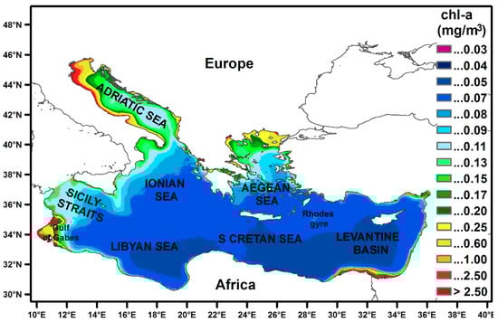
Figure 1.
The study area (Eastern Mediterranean Sea) along with the mean yearly chlorophyll climatology as computed from the Copernicus Marine Environment Monitoring Service (CMEMS) data for the period 1998–2016.
The chlorophyll data used were the Copernicus Marine Environment Monitoring Service (CMEMS) product OCEANCOLOUR_MED_CHL_L4_REP_OBSERVATIONS_009_078; these involve the reprocessed surface chlorophyll concentrations (at a 1 km resolution) from multi-satellite observations (SeaWiFS, MODIS-Aqua, MERIS, and VIIRS sensors). This CMEMS product is developed based on regional ocean color algorithms that differentiate between case-1 and case-2 waters [33,34,35,36]. The applied algorithms have increased the accuracy of the resulting products, especially for the low chlorophyll values that characterize the major part of the E Med. It is noted that surface chlorophyll concentrations derived with the use of global ocean color algorithms over-estimated the Med’s low chl-a in situ field and were characterized by an absolute percentage difference from the in situ observations that exceeded 100%. The use of the regional-Med algorithm MedOC4 [35] significantly reduced these over-estimations and resulted in absolute percentage differences below 50% from the in situ field. As a consequence, for a study like as the present one that focuses on the oligotrophic E Med waters, this chlorophyll product is considered the most suitable. The environmental data of the study were the numerical products of the European Centre for Medium-Range Weather Forecasts (ECMWF) ERA Interim reanalysis; their spatial resolution is approximately 80 km, but they can be retrieved bilinear interpolated at 0.125°. Specifically, the data retrieved were: the monthly means of daily means for 10 m wind speed, MSL pressure, and SST; the monthly means of daily forecast accumulations for precipitation; and the four analyses per day of the significant height of combined wind waves and swell that were used for computing its monthly means. It is noted that the major part of this study was performed in the framework of a Geographic Information System (GIS).
Monthly averages, as in other studies [5,15,30], were computed for all variables in a 1° × 1° grid of the study area for the study period; that is, 158 points covering the E Med Sea with 216 values each. It should be noted that such a coarse analysis was selected for several reasons: the present study was mainly focused on the open sea oligotrophic area, the absolute percentage errors even of the most suitable chlorophyll product used were still quite large and the native resolution of the numerical model was small. Consequently, the results were more accurate for the open sea that is characterized by less abrupt changes in chlorophyll concentrations. Means of the parameters were also calculated for each month in order to produce the monthly climatology. Based on this climatology for chlorophyll concentrations that is presented in Appendix A, the year was separated into two periods: the “high production period” (November–April) and the “low production period” (May–October) characterized by higher and lower chlorophyll values, respectively; the mean values for these periods were also computed for each year. The above is consistent with the study of Salgado-Hernanz et al. [32] where chlorophyll peaks were identified for the E Med from January to April and the initiation of chl-a growing period was not found before November even for areas of a highly possible secondary bloom in autumn.
Data’s seasonality was removed by subtracting each month’s climatology value from the mean monthly value to produce the “anomalies” of the parameters, as is usually implemented [11,16]. The maximum anomalies observed for the parameters during the study period were checked in order to define the extent of their variations.
The selected parameters (SST, 10 m wind speed, wave height, precipitation, and MSL pressure) with respect to their possible influence on chl-a are described in the introduction section. It is noteworthy that the wave height was also selected here, as it is an environmental factor that is quite similar to the wind but has a greater ability to describe the wind-mixing potential. The significant wave height for a fully developed sea is proportional to the second power of wind speed [37], quite similar to the wind stress, which mainly determines the wind-mixing and upwelling procedures [15]. According to the authors’ knowledge, the wave height is studied here for the first time as an environmental parameter possibly related to chlorophyll concentration.
For detecting possible relationships between surface chl-a and the selected environmental parameters, the correlations between their anomalies were calculated. Although correlations do not ensure a cause–effect relationship, they can be used together with other findings to reach useful conclusions. Chlorophyll data, as well as other parameters’ data (especially for precipitation), were not normally distributed for several points. Since the Spearman rank correlation coefficient is quite unaffected by the data distribution (as well as by outliers), it was selected for estimating the correlations between the anomalies of chl-a and the examined environmental factors. These correlations were calculated for all data and separately for the data of the high production period (November–April) and the low production period (May–October); they were also extracted on a seasonal basis for winter (December–February), spring (March–May), summer (June–August), and autumn (September–November). Their values were considered low (small) up to 0.3, moderate between 0.3 and 0.5, and strong (high) when exceeding 0.5. They were considered significant at a confidence level >95% (p-value < 0.05) and only the relevant results are presented.
Chlorophyll trends were computed for the mean values of the high and the low production periods of each year. The idea for such a discrimination originated from the study of Coppini et al. [29] where a chl-a trend calculation was conducted for the summer (May–September) period aiming toward the development of an indicator for eutrophication based on ocean color data that monitors eutrophication trends. In addition, the above mentioned feature differentiates the present study from the several others addressing this topic. First, Spearman rank correlation was applied in order to detect the points presenting significant trends at a confidence level of 95%. Then, for these points, the linear trend was estimated. Trends of the environmental factors examined were also calculated for the time period studied and with the same method for comparison purposes. It is noted that, Spearman rank correlation has been identified as a useful tool for detecting trends with time, giving quite similar results with the Mann–Kendall test [38,39], while linear trends are, in general, estimated [11,31].
3. Results
The main characteristics of the monthly climatology for the E Med Sea, as computed from the CMEMS monthly product for the period 1998–2016 (Appendix A) were: the ultra-oligotrophic condition of the southern open sea and especially of the Levantine Basin, which was extremely enhanced during July, August, and September; the highest chl-a values of the NW Adriatic, the gulf of Gabes, and the Nile river plume (NE Africa) coastal regions, which were maintained all year long; the more “productive” regions of the W Libyan Sea, the Sicily Straits, the Adriatic Sea, the W Ionian Sea, and the N Aegean; the Rhodes gyre, which was strongly shown through the monthly climatology during spring; and the specific behavior of the southern Adriatic gyre, which had lower chl-a values than the nearby regions throughout the year, except for March when it showed higher values, presenting blooming characteristics. In general, the E Med was characterized by a high production period that extended from November to April when the higher chlorophyll concentrations were observed (the highest were observed in February for most of the areas) and a low production one from May to October; the chlorophyll climatological mean values for these two periods are given in Figure 2.
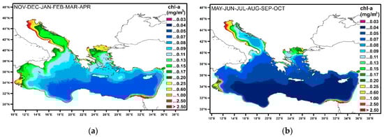
Figure 2.
Chlorophyll climatology for the high (a) and the low (b) production periods as computed from the CMEMS data for the period 1998–2016.
During the high production period (November–April): SST presents a N–S increasing gradient of 12.4–19.6 °C; the stronger winds were found over the western open sea area, but also in the Aegean; higher waves were present over the open sea, especially over its western part and mainly in the Ionian; lower precipitation amounts were observed over the southern part of the study area, while the Adriatic Sea, the Ionian Sea, the E Aegean, and the northern and eastern parts of the Levantine Basin presented higher values. During the low production period (May–October): SST ranged from 20.0 to 26.3 °C, with the higher values encountered in the E Levantine Basin; stronger winds were found in the Aegean; the area extending from the central Aegean down to Africa was characterized by higher waves; the precipitation was much lower and its higher values were found in the Adriatic, the E Ionian, and the N Aegean. All the above were derived from the relevant climatology which was computed with the use of the ERA Interim dataset for the period 1998–2016 and they are shown in Appendix B for the 158 points studied here.
3.1. Chlorophyll Correlations with Environmental Factors
The Spearman rank correlation coefficients between the monthly anomalies of chl-a and the environmental factors of SST, 10 m wind, wave height, and MSL pressure are presented here. It is worth mentioning the maximum anomalies of the examined parameters throughout the study period, which were calculated as a measure of their variability. Chlorophyll anomalies (Figure 3), presented their higher values over the Adriatic and the N Aegean Seas, as well as for several near-shore points, exceeding 80% and even 100% of the climatological mean value. For the open sea, they usually ranged between 20 and 60% of the climatological mean depending on the season (and for a few points between 10 and 20%, especially during summer); however, they were larger for the spring period ranging between 30 and 80% of the climatological mean value and even exceeding it, especially for points of the Rhodes gyre region and the Sicily Straits. SST presented lower anomaly values in winter and spring seasons, ranging from 0.5 to 1.5 °C; for the summer and autumn periods, the anomalies were found to be higher over the western and the eastern parts of the study area, respectively, exceeding 2 °C in many places. Wind anomalies were found to be 10–40% of the climatological mean with a few exceptions up to 50% for all seasons. Wave height anomalies were found to be 30–70% of the climatological value for the winter period, while for the other seasons, they were smaller, except for the N Aegean during summer. They presented their higher values for the Adriatic and the Aegean Seas, and the lower ones over the southern open sea and especially its central parts. Precipitation was the parameter with the greatest anomalies; they exceeded 50% of the climatological mean in all seasons, while over large areas, they were 2–3-fold greater that the climatological average, even during the low production period when the E Med is characterized by low rainfall amounts. MSL pressure anomalies presented a NW–SE decreasing gradient. For the high production period and especially during winter when the higher values were observed, they exceeded 10 hPa over the N Adriatic Sea and went down to 4 hPa over the eastern parts of the Levantine Sea. For the low production period, the anomalies were much smaller, with a higher value of 5 hPa observed for the N Adriatic in October. The amplitude of the parameters’ observed anomalies showed that it was worth studying their relations.
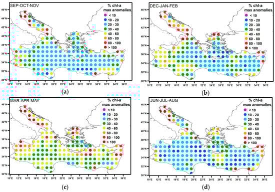
Figure 3.
Maximum chlorophyll anomalies observed each season for the time period 1998–2016 for: (a) autumn, (b) winter, (c) spring, (d) summer.
For the high production period, the significant correlations between chl-a and SST were all found to be negative and referred to the majority (81.6%) of the points (Figure 4a); only the N Adriatic Sea, the north and east Aegean parts, and several near-shore points were excluded. They were higher, even reaching −0.7, for the open sea (SSW part of the study area), i.e., excluding the eastern Levantine Basin, which presented low to moderate correlations. For the low production period, the points that presented a significant relation between the two parameters were much fewer (53 out of 158), while four of these points even presented positive correlations (over the gulf of Gabes and the eastern part of the Levantine Basin). During this period, the observed negative correlations were small in general (up to −0.4), and they were mainly observed over the northern parts of the study area (Adriatic, E Ionian, and Aegean Seas) (Figure 4b). The seasonal-based calculations are presented in Figure 5. In autumn, 68 out of the 158 points presented significant negative correlations of chl-a and SST, with moderate to high values for the central parts of the study area (SE Adriatic, E Ionian, Aegean, S Cretan, W Levantine, and E Libyan Seas). During winter, 80 points were found with statistically significant negative correlations between the two parameters, presenting moderate to strong relationships over the south and mainly the southwest parts of the E Med; this was especially true for the Libyan Sea where the correlations were up to −0.7. However, seven points with positive correlations were also found over the SE Aegean and the N Levantine near-shore regions. Spring was characterized by moderate and strong relationships between chl-a and SST for most (88%) of the E Med, mainly excluding the N Adriatic and the northern Aegean. For the summer period, 10 points out of 158 presented negative correlations and 12 points presented positive ones; low negative correlations characterized 43% of the Adriatic Sea and three points of moderate negative relationships were found over the E Levantine Basin, while the points presenting positive correlations were mainly found near the gulf of Gabes. The inverse relation between chl-a and SST was clear, characterized at almost every part of the E Med Sea depending on the season, except for summer, and it was more pronounced in spring. This inverse relationship was also observed for the data throughout the year for 135 out of 158 points that presented statistically significant correlations, especially over the central parts of the south E Med (Figure A3a), i.e., the W Libyan, the S Cretan, and the E Levantine Seas.
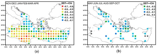
Figure 4.
Spearman rank correlation coefficients between chl-a and SST monthly anomalies for the high (a) and the low (b) production periods. Only significant correlations are shown.
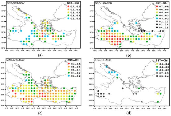
Figure 5.
Spearman rank correlation coefficients between chl-a and SST monthly anomalies on a seasonal basis: (a) autumn, (b) winter, (c) spring, and (d) summer. Only significant correlations are shown.
Chlorophyll and 10 m wind speed correlations were found to be positive and significant for 111 out of the 158 points during the high production period (November–April) over the southern parts of the study area and larger for the central parts (E Libyan and S Cretan Seas) where they were moderate to strong (Figure 6a). For the low production period (May–October), the correlations were very few and low, with 17 points presenting significant values and 5 of them negative ones (Figure 6b). When data throughout the year were considered, the results were similar to the ones of the high production period, with 102 points presenting statistically significant positive relationships, but with lower correlations (Figure A3b). The seasonal results are shown in Figure 7. For the autumn period, only 18 out of the 158 points were found with significant and positive correlations between the two parameters, mainly over the E Libyan Sea and the west part of S Cretan Sea with moderate values. The majority of the points (102 out of 158) presenting significant and positive correlations between chl-a and 10 m wind speed were found in winter. They were mainly observed over the southern part of the study area and the higher values (up to 0.8) were found for the S Cretan Sea. In spring, 36 points presented low to moderate positive correlations and their moderate values were found over the S Cretan Sea and the eastern part of the Levantine Basin. For the summer period, only 2 points were found with positive correlations and 10 with negative relations between the two parameters; the latter were mainly found over the southern part of the study area. In conclusion, positive significant correlations between chl-a and 10 m wind speed were calculated for the south seas, excluding summer, and were mainly found in winter, with the S Cretan Sea presenting the higher values.
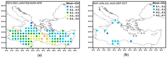
Figure 6.
Spearman rank correlation coefficients between chl-a and 10 m wind speed monthly anomalies for the high (a) and the low (b) production periods. Only significant correlations are shown.
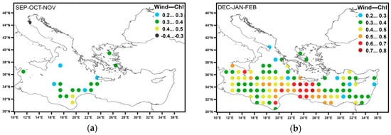
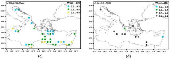
Figure 7.
Spearman rank correlation coefficients between chl-a and 10 m wind speed monthly anomalies on a seasonal basis: (a) autumn, (b) winter, (c) spring, and (d) summer. Only significant correlations are shown.
The correlations of chl-a and wave height for the high production period (Figure 8a) were found to be positive and significant over a major part (88%) of the area, i.e., for 139 out of the 158 points. The higher values were calculated for the southern part of the area and mainly in its central parts (E Libyan, S Cretan, and W Levantine regions) where they were moderate to strong, while the Adriatic Sea presented moderate correlations over its eastern and southern parts. During the low production period (Figure 8b), the positive correlations were few (30 points) and lower, with the S Adriatic and the N Ionian forming a compact region of quite high (up to 0.4) values. The seasonal results for the correlations between wave height and chlorophyll are shown in Figure 9. For the autumn period, 75 out of the 158 points presented low to moderate positive correlations; their moderate values were mainly found over the south-central part of the study area (E Libyan and western parts of S Cretan and W Levantine regions) and the Aegean Sea. For the winter season, the correlations were like the ones of the high production period but with higher values: 135 points presented significant correlations and only 11 of them presented low values; 47 of these points over the southern part of the sea were characterized by strong correlations, especially over the S Cretan Sea where the values were up to 0.8. In spring, 69 points were found with positive correlations presenting higher values for the southern part of the study area and the Adriatic Sea, while stronger correlations (up to 0.6) were observed for the central Adriatic Sea and the southern part of the Levantine Basin. For the summer period, the correlations over the southern parts of the area resulted in negative values for 29 points, and only parts of the Adriatic, the N Ionian and the E Levantine presented low to moderate positive values (13 points in total). The year-round results (Figure A3c) were like the ones found for the high production period but with lower values, with 136 points presenting positive correlations and up-to-moderate values found for the central Adriatic Sea and the south-central parts of the study area (E Libyan Sea, S Cretan Sea, and locally over the Levantine Basin). These correlations, compared to the ones between chl-a and 10 m wind speed, presented similar patterns but resulted in higher values and included more parts of the study area, especially the Adriatic Sea.
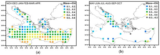
Figure 8.
Spearman rank correlation coefficients between chl-a and wave height monthly anomalies for the high (a) and the low (b) production periods. Only significant correlations are shown.
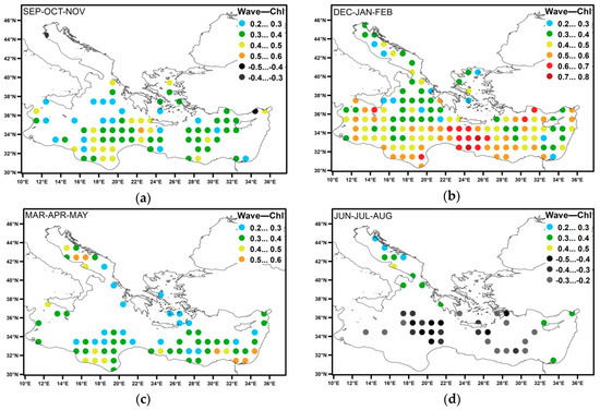
Figure 9.
Spearman rank correlation coefficients between chl-a and wave height monthly anomalies on a seasonal basis: (a) autumn, (b) winter, (c) spring, and (d) summer. Only significant correlations are shown.
Chlorophyll and precipitation were found to be positively correlated. Low to moderate correlations were calculated for the high production period (November–April) for 62 out of the 158 points over the SSW parts of the study area, especially over the Levantine Basin, near the Sicily Straits and locally over the Adriatic Sea (Figure 10a). For the low production period (May–October) these positive correlations (observed for 123 points) covered a wide part of the E Med, mainly with the exception of the SW and SE parts; their values showed moderate correlations, with the higher ones (0.4–0.5) for the S Adriatic, the Ionian, the E Libyan, and the S Cretan Seas (Figure 10b). When data throughout the year were considered (Figure A3d), the positive correlations referred to 111 points and they were low in general with a few exceptions of moderate values, mainly for the Levantine Sea. According to the seasonal results (Figure 11), moderate to strong (up to 0.6) positive correlations were found for the central and the southern Adriatic Sea in the spring and summer periods and locally over the N Aegean in the autumn–winter period. The open sea presented low to moderate correlations: over the Ionian in autumn and its west part during summer; locally over the Libyan Sea during all seasons except winter, mainly in summer; over the S Cretan Sea in winter; and the Levantine Sea presented such values during all seasons except summer, mainly in winter. For the winter season and for the other seasons, 63 and 38 out of the 158 points, respectively, were found to present positive relationships between chlorophyll and precipitation. In conclusion, positive significant correlations between chl-a and precipitation were calculated for the eastern parts in winter and for the western parts during the other seasons, mainly in summer.
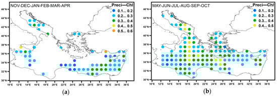
Figure 10.
Spearman rank correlation coefficients between chl-a and precipitation monthly anomalies for the high (a) and the low (b) production periods. Only significant correlations are shown.
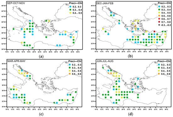
Figure 11.
Spearman rank correlation coefficients between chl-a and precipitation monthly anomalies on a seasonal basis: (a) autumn, (b) winter, (c) spring, and (d) summer. Only significant correlations are shown.
Stronger correlations between chl-a and the environmental parameters were found over the southern open sea, where the results of this study can be considered more accurate due to the coarse analysis. They were negative for chlorophyll and SST over the SW part in winter and all southern parts in spring, and positive between 10 m wind speed and wave height with chl-a over the central S parts and all southern parts, respectively, in winter. Quite interesting were the negative low to moderate correlations between chl-a and wave height that were observed for several points in summer. The correlations of chlorophyll with precipitation were up to moderate and they were found to the eastern part in winter and to the west part during the other seasons. The high production period was characterized by the correlations of chl-a with SST, 10 m wind speed and wave height, while the correlations between chlorophyll and precipitation were present mainly during the low production period, except for the S Levantine parts where they were observed for the high production period.
The correlations between chl-a and MSL pressure were very few in general, low and scattered for the low production period and the seasons of spring, summer, and autumn (not shown). The winter season (Figure 12a) presented significant negative correlations for 58 out of the 158 points; moderate to strong correlations over the western parts of the study area, near the Sicily Straits and locally over the Adriatic and the Ionian Seas; and up to moderate correlations over the S Cretan Sea, the N Levantine Sea, and at places in the Aegean. The correlations were fewer (they referred to 23 points) and lower when all the high production period was considered, with their higher values mainly near the Sicily Straits (Figure 12b).
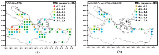
Figure 12.
Spearman rank correlation coefficients between chl-a and MSL pressure monthly anomalies for the high production period (a) and for the winter season (b). Only significant correlations are shown.
3.2. Chlorophyll Trends
All significant surface chlorophyll trends, as calculated for the period 1998–2016, based on the mean chl-a values of each year and separately for the high and the low production periods were found to be positive. They are shown in Figure 13 as percentages of their respective climatological value per year. The Adriatic Sea presented positive chl-a trends for the high production period (1–2% of the climatological value per year). For both the high and the low production periods, significant trends were found for the area near the Sicily Straits (with greater values, 1–2% of the climatological value per year, for the high production period) and the central and south Aegean parts (ranging in general from 0.5 to 1% of the climatological value per year), as well as to a few points of the Ionian and the Libyan Seas. The the S Cretan and the Levantine Seas presented increasing chl-a trends, mainly for the low production period (0.5–1% of the climatological value per year in most cases). In summary: during the high production period, 35 out of the 158 points presented statistically significant increasing trends, up to 2.8% of the climatological value per year, and mainly characterized the western part of the E Med; for the low production period, the significant trends were observed for more points (58 out of 158), they were again all increases of 0.4–2.5% of the climatological value per year, and they were mainly found in the eastern part of the study area.
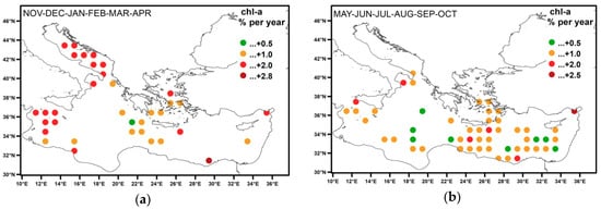
Figure 13.
Chlorophyll trends (% of the climatology per year) during 1998–2016 for the high (a) and the low (b) production periods. Only significant trends are shown.
For the same time period, the trends of the environmental factors SST, 10 m wind speed, wave height, and precipitation are presented in Appendix D. SST presented an increasing trend over a large part of the Ionian Sea for the high production period and over the southern part of the Levantine Sea for both periods (Figure A4). These areas were characterized by the absence of a correlation or low correlation between SST and chl-a, and only locally coincide with increasing chl-a trends. For the wave height, a large area of positive trends was found for both periods over the Adriatic Sea, the Ionian, the west part of the Cretan Sea, the N Aegean, and the northern part of the Levantine Sea; a negative trend was calculated for the SE Aegean (Figure A5). Over the Adriatic Sea, chl-a presented an increasing trend, and for this area, the correlations between wave height and chlorophyll were moderate mainly during the high production period; similar was the case locally over the Ionian Sea and over the western part of the S Cretan Sea where the two parameters presented strong correlations for the high production period (November–April); over the N Aegean, no increasing trend was found for chlorophyll and its correlations with wave height were found to be low; over the north Levantine Basin, chlorophyll did not show an increasing trend, while the relevant correlations were moderate; over the SE Aegean, where the wave height showed a negative trend, chl-a presented a positive one, and the correlations between them were found to be negative or absent for the low production period. Precipitation and 10 m wind speed did not present significant trends for the high production period. For the low production period, wind presented an increasing trend for the S Adriatic, the Ionian, and locally over the E Levantine, as well as a decreasing one for the SE Aegean (Figure A6a); for these regions, no correlation with chl-a was found. A positive trend for precipitation was calculated for the central Adriatic, the E Ionian, the W Aegean, the S Cretan, and the N Levantine (Figure A6b). The similar trends for chlorophyll coincide only for the S Cretan Sea where up to moderate positive correlations with precipitation were found. For the majority of the points where chlorophyll trends were met together with trends of other parameters, the results did not contradict- their estimated correlations.
In Appendix E, the chlorophyll concentrations for the high and the low production periods of November 1998–April 1999, November 2015–April 2016, May–October 1998, and May–October 2016 are given in order showing changes in concentrations based on ocean color data, which can be compared to in situ observations.
4. Discussion
4.1. Correlations among Chlorophyll and Environmental Variables
The SST presented an inverse significant relationship with chl-a, which characterized the major part of the study area during the high production period and in spring; this relation was minimized and even inversed in summer. In the study of Katara et al. [16] for the whole Mediterranean Sea, it was found as a preliminary result that all statistically significant correlations between chl-a and SST were negative. The two parameters were also found to be negatively correlated for the Aegean basin [40] and an inverse relation between them was revealed for specific areas of the E Med [19]. This kind of relationship supports the outcome that the strength of stratification, as inferred from the SST, is a major controller of phytoplankton abundance for the nutrient-limited Med Sea. Higher SSTs, representing stronger water column stratification, produce reduced vertical mixing and low nutrient amounts for the surface layer leading to low chl-a concentrations. Such a relation between SST and chl-a was detected for the non-blooming and the intermittently-blooming areas of the entire Med, such as the ones of its eastern part (i.e., the whole Basin except for some coastal parts) [12]. The results found here gave further evidence for the above through the higher inverse correlation of the parameters during the transitional periods of spring and autumn (for the northern part), when the mixed layer begins to become shallow or deepen, respectively [13,41]. With lower SST values denoting a deeper MLD, the later MLD starts to decrease in spring and the sooner it starts to increase again in autumn, the larger the positive influence it can have on phytoplankton, as seen through chlorophyll concentrations. This was also the case for the SSW part of the study area during winter, according to the MLD of the region. In addition, for the winter season (for the northern part) characterized by the deepest MLD and for the summer when the shallowest MLD was observed [13,41], the relative correlations were absent. Furthermore, the inverse correlation between SST and chlorophyll was minimized and even reversed for the summer season, showing the marginal or absent effects of SST decreases in an already nutrient-poor environment. It should also be noted that, although such an inverse relationship was anticipated between SST and chlorophyll or net primary production for the larger part of the oceans [24,27], this was not always the case, even for the Med. The two parameters were found presenting opposite trends for the major part of the E Med Sea for the period 1999–2004 in the global study of Behrenfeld et al. [24]. However, areas showing decreases in both SST and net primary production were also found in the same study, especially over the Levantine Basin. For the same time period, the results for the E Med showed decreases in SST along with both positive and negative variation for chlorophyll in another global study [27]. For a longer interval, December 2002–January 2015, the E Med was found to have increases for both chl-a and SST [28]. The latter studies point to the conclusion that SST alone cannot describe chl-a variations [28].
The significant correlations between chlorophyll and 10 m wind speed were all found to be positive (with the exception of a few points during summer). This positive relation of the parameters mainly characterized the southern parts of the E Med for the high production period and the winter season. The mechanism behind these positive correlations is the wind-induced mixing, which by deepening the MLD, could result in increased nutrient fluxes from the deeper layers to the surface, and as a consequence, to increased chlorophyll concentrations. Such correlations were found for the two parameters in the Med [16] and this inverse relationship was also identified for the Rhodes Gyre area [19]. The most relevant study was the global one of Kahru et al. [15] for the period November 1996–October 2009 on correlations between chlorophyll and wind satellite data throughout the year, which resulted in a similar pattern with the one of the present study: all the significant correlations were found to be positive and they were also mainly recorded over the southern open sea. In addition, the same areas as here were characterized by the higher correlations and comparable values were observed; however, more areas over the Levantine Basin were found to have significant correlations [15]. In the above-mentioned study [15], such correlations were found for areas with relatively shallow MLDs and nutrients were pointed out as the main limiting factor for phytoplankton growth. This was also the case here for the winter season when the MLD over the southern E Med is, in most parts, shallower than the one of the northern parts [13,41]; it is more likely for the wind mixing to deepen a shallower MLD, resulting in more available nutrients for the surface layers. The opposite result was observed during summer, when the deepening of the MLD decreased chl-a [15]. The few positive correlations between wind and chlorophyll that were found here for the summer period could be explained this way. Since the area is characterized by a deep chlorophyll maximum during this season [42], any deepening of the MLD could only diffuse the limited available nutrients leading to chl-a decreases or to a redistribution of the chlorophyll content down to depths where it is not detected by the ocean color measurements. The absence of correlations between chl-a and wind in the summer period over the Aegean Sea was also consistent with the results of other studies [40,43]. The prevailing summer winds in the Aegean Basin are northerlies and cause upwelling events over its eastern part that do not influence surface chlorophyll concentrations [40,43]; although the present study dealt with the wind speed and not with its direction, no significant correlations of the two parameters were found. All significant correlations between wave height and chlorophyll were positive (except for several points over the S Med during summer). This relationship mainly characterized the high production period and the winter season. In general, these correlations presented, as expected, similar patterns with the ones between wind and chlorophyll. However, their values were higher and more points presented significant positive correlations over the northern parts of the E Med and mainly for the Adriatic Sea. The number of points with significant negative relations between the parameters, for the summer period over the southern part of the study area, were also higher. The mechanism through which higher waves can result in increased chlorophyll concentrations (and decreased ones during summer) are the same as for the wind speed described above. Nevertheless, the wind influence on the sea surface can be better described through the wave height, especially for non-open seas, such as the Adriatic and the Aegean Seas; wind needs fetch to produce higher waves that can mix the water column. In addition, the waves respond to the wind stress, which better describes the wind mixing and upwelling procedures [15]. The results of the wave–chlorophyll correlations found here, which included more areas with significant results than the ones of the wind–chlorophyll relation, point to the conclusion that the wave height is more suitable than the wind speed, especially in cases of non-open sea areas, in studying possible relations with chl-a concentrations.
The significant correlations between chlorophyll and precipitation were all positive and were mainly found during the low production period, with the exception of the southern parts of the Levantine Basin, which presented such correlations in the high production period; in general, low to moderate values were found. An exception of moderate to strong positive correlations was found in the central and southern Adriatic Sea in the spring–summer period. The eastern parts of the study area presented these correlations in winter, while the western parts presented them in the other seasons, mainly in summer. Positive correlations between these parameters were found in the Med Sea [16] and larger precipitation amounts were related with higher chlorophyll values in specific areas of the E Med [19]. Considerable short-lived chl-a increases were recorded after extreme rainfall events during the early autumn and summer periods over the Hellenic Seas and mainly for the E Ionian and the N Aegean Seas; they were attributed to the atmospheric deposition of nutrients into the sea [21,22]. It is noted that the atmosphere was identified as an additional nutrient source for the E Med [23], especially during the low production period; the relevant correlations found here characterize a wide area during this period. In addition, the study area is subject to dust deposition that was found to be positively correlated with chlorophyll [44], and in its wet form can result in significant chl-a increases [45,46].
MSL pressure and chlorophyll were found to have significant negative correlations over quite a large area only for the winter season, mainly over the western part of the E Med where these correlations were larger. It is noted that MSL pressure monthly anomalies also had higher values over the western part where the majority of these correlations were found. One could argue that the areas presenting significant inverse correlations between the two parameters are also affected by deep barometric lows [25] that induce strong winds and high rainfall amounts.
4.2. Temporal Trends in Chlorophyll Concentrations
All the significant surface chlorophyll trends, estimated separately for the high and the low production periods of 1998–2016, were found to be positive. They mainly characterized the western part of the study area during the high production period and the eastern part for the low production period. They were not contradictory to the trends of the other parameters when seen together with their relevant correlations.
In a recent study of the same time period, only increasing chlorophyll trends were found [31]. Despite the different approaches followed, i.e., the present study was conducted using a much coarser analysis and it discriminated between the high and the low production periods, similar results in defining both the areas presenting significant trends and the trend magnitude were found. The results here, compared to another long-term study of Salgado-Hernanz et al. [32] for the time period 1998–2014, were in partial agreement regarding the increasing chlorophyll trends in the Adriatic Sea and the Sicily channel. On the other hand, in the above-mentioned study [32], a low decreasing trend was found for the rest of the E Med, which was not observed in the present work. For the E Med, the results of several studies presented considerable differences: mainly decreasing chlorophyll trends were found for 1998–2003 [11]; from 1979–1983 to 1998–2002 increasing trends for both SST and chl-a were observed, while for 1999–2004, a decreasing trend for SST along with increasing and decreasing chlorophyll trends were found [27]; for the May–September period of 1998–2009, positive and negative chl-a trends were calculated [29]; both decreasing and increasing chl-a trends were estimated for the period 1998–2009, along with much greater trend magnitudes [30]; and only increasing trends for both chl-a and SST were found for December 2002 to January 2015 [28], similar to the present study. Such different estimations were also found in studies referring to other parameters, i.e., for SST trends [27,28,47] and precipitation trends [48,49], when comparing them and in respect to the present work. However, for SST, most of them resulted in increasing trends [28,47]. The results of the studies mentioned above [11, 27-32] were described so briefly because it is obvious that the trend estimation is highly dependent on the time period studied. Much longer time series are needed for the detection of trends in order to reach safer results, exceeding 30 years, which is the usual practice for meteorological parameters; this has also been proposed for phytoplankton’s climate-driven trends [50].
Regarding environmental variables’ future changes that have been predicted by climate models for the Med, e.g., an increase for SST [47] and a decrease in precipitation [14,49], it is crucial to reveal the possible relations between these variables and chlorophyll concentrations. The estimation of the relevant correlations can unveil aspects of these relations. According to the results of the present study, the predicted future increase in SST and decrease in precipitation mentioned above could lead to chlorophyll decreases. However, the respective studies are quite scarce, especially for precipitation, upon which more work needs to be done. In addition, studies over long time series, such as the one conducted here, but with higher spatial resolution, are proposed. As far as the chlorophyll trends are concerned, which have been more extensively studied with controversial results, longer and more homogenous time series are required to be built.
5. Conclusions
The main results of this work can be summarized for the study area of the E Med and the period 1998–2016 as follows: SST was inversely related to surface chl-a in the major part of the Sea; this relation was more pronounced in spring and not valid for the summer season. Wind speed and mainly wave height were positively correlated with chlorophyll, especially over the southern open part of the Sea; however, during the summer period, a negative relation was observed. For precipitation and chl-a, all the significant correlations were positive and mainly valid for the low production period. MSL pressure and chl-a presented significant negative correlations for the winter season and mainly over the western part of the Sea. All the significant surface chlorophyll trends were found to be positive; nevertheless, the trend estimation requires much longer time series than the available ones.
Author Contributions
Conceptualization, D.K. (Dionysia Kotta); Data curation, D.K. (Dionysia Kotta); Formal analysis, D.K. (Dionysia Kotta); Investigation, D.K. (Dionysia Kotta); Methodology, D.K. (Dionysia Kotta); Project administration, D.K. (Dionysia Kotta) and D.K. (Dimitra Kitsiou); Resources, D.K. (Dionysia Kotta); Supervision, D.K. (Dionysia Kotta) and D.K. (Dimitra Kitsiou); Validation, D.K. (Dionysia Kotta) and D.K. (Dimitra Kitsiou); Visualization, D.K. (Dionysia Kotta); Writing–original draft, D.K. (Dionysia Kotta); Writing–review and editing, D.K. (Dionysia Kotta) and D.K. (Dimitra Kitsiou).
Funding
This research received no external funding.
Acknowledgments
Copernicus Marine Environment Monitoring Service and ECMWF are acknowledged for the data.
Conflicts of Interest
The authors declare no conflict of interest.
Appendix A
The monthly chlorophyll climatology, as computed for the 1998–2016 time period, is given here.


Figure A1.
Chlorophyll monthly climatology as computed for the period 1998–2016 for January to December (a–l).
Appendix B
The climatology of the high and the low production periods for SST, 10 m wind speed, and precipitation as computed with the use of the ERA Interim dataset for the period 1998–2016 is shown in this appendix.


Figure A2.
SST (a,b), 10 m wind speed (c,d), wave height (e,f), and precipitation (g,h) climatology for the period 1998–2016 of the 158 points studied here for the high (November–April) and the low (May–October) production periods, respectively, as derived from the ERA Interim data set.
Appendix C
Spearman rank correlation coefficients between the monthly anomalies of chl-a and the environmental factors examined on a yearly basis are presented in this appendix.

Figure A3.
Spearman rank correlation coefficients throughout the year between the monthly anomalies of chl-a with: (a) SST, (b) 10 m wind speed, (c) wave height, and (d) precipitation. Only significant correlations are shown.
Appendix D
The trends of the environmental factors of SST, 10 m wind speed, wave height, and precipitation for the period 1998–2016 are given here. It is noted that these results are not representative for climate studies since they refer to a limited time period.

Figure A4.
SST trends (°C per year) during 1998–2016 for the high (a) and the low (b) production periods. Only significant trends are shown.

Figure A5.
Wave height trends (% of the climatology per year) during 1998–2016 for the high (a) and the low (b) production periods. Only significant trends are shown.

Figure A6.
The 10 m wind (a) and precipitation (b) trends (% of the climatology per year) during 1998–2016 for the low production period. Only significant trends are shown. For the high production period, no significant trends were detected.
Appendix E
The chlorophyll concentrations for the high and the low production periods of November 1998–April 1999, November 2015–April 2016, May–October 1998, and May–October 2016 are given in this appendix for comparison purposes.

Figure A7.
Chlorophyll concentrations for the high production periods of November 1998–April 1999 (a) and November 2015–April 2016 (b), and the low production periods of May–October 1998 (c) and May–October 2016 (d).
References
- Field, C.B.; Behrenfeld, M.J.; Randerson, J.T.; Falkowski, P. Primary production of the biosphere: Integrating terrestrial and oceanic components. Science 1998, 281, 237–240. [Google Scholar] [CrossRef] [PubMed]
- Vargas, C.A.; Escribano, R.; Poulet, S. Phytoplankton food quality determines time windows for successful zooplankton reproductive pulses. Ecology 2006, 8, 2992–2999. [Google Scholar] [CrossRef]
- Gregg, W.W.; Conkright, M.E.; Ginoux, P.; O’Reilly, J.E.; Casey, N.W. Ocean primary production and climate: Global decadal changes. Geophys. Res. Lett. 2003, 30, 1809. [Google Scholar] [CrossRef]
- Hays, G.C.; Richardson, A.J.; Robinson, C. Climate change and marine plankton. Trends Ecol. Evol. 2005, 20, 337–344. [Google Scholar] [CrossRef] [PubMed]
- Feng, J.; Durant, J.M.; Stige, L.C.; Hessen, D.O.; Hjermann, D.Ø.; Zhu, L.; Llope, M.; Stenseth, N.C. Contrasting correlation patterns between environmental factors and chlorophyll levels in the global ocean. Glob. Biogeochem. Cycles 2015, 29, 2095–2107. [Google Scholar] [CrossRef]
- Maritorena, S.; Siegel, D.A. Consistent merging of satellite ocean color data sets using a bio-optical model. Remote Sens. Environ. 2005, 94, 429–440. [Google Scholar] [CrossRef]
- Joint, I.; Groom, S.B. Estimation of phytoplankton production from space: Current status and future potential of satellite remote sensing. J. Exp. Mar. Bio. Ecol. 2000, 250, 233–255. [Google Scholar] [CrossRef]
- Turley, C.; Bianchi, M.; Christaki, U.; Conan, P.; Harris, J.; Psarra, S.; Ruddy, G.; Stutt, E.; Tselepides, A.; Van Wambekeet, F. Relationship between primary producers and bacteria in an oligotrophic sea--the Mediterranean and biogeochemical implications. Mar. Ecol. Prog. Ser. 2000, 193, 11–18. [Google Scholar] [CrossRef]
- D’Ortenzio, F.; Ribera D’Alcalà, M. On the trophic regimes of the Mediterranean Sea: A satellite analysis. Biogeosciences 2009, 6, 139–148. [Google Scholar] [CrossRef]
- Karydis, M.; Kitsiou, D. Eutrophication and environmental policy in the Mediterranean Sea: A review. Environ. Monit. Assess. 2012, 184, 4931–4984. [Google Scholar] [CrossRef]
- Barale, V.; Jaquet, J.M.; Ndiaye, M. Algal blooming patterns and anomalies in the Mediterranean Sea as derived from the SeaWiFS data set (1998–2003). Remote Sens. Environ. 2008, 112, 3300–3313. [Google Scholar] [CrossRef]
- Volpe, G.; Nardelli, B.B.; Cipollini, P.; Santoleri, R.; Robinson, I.S. Seasonal to interannual phytoplankton response to physical processes in the Mediterranean Sea from satellite observations. Remote Sens. Environ. 2012, 117, 223–235. [Google Scholar] [CrossRef]
- D’Ortenzio, F.; Ludicone, D.; de Boyer Montegut, C.; Testor, P.; Antoine, D.; Marullo, S.; Santoleri, R.; Madec, G. Seasonal variability of the mixed layer depth in the Mediterranean Sea as derived from in situ profiles. Geophys. Res. Lett. 2005, 32, L12605. [Google Scholar] [CrossRef]
- Giorgi, F.; Lionello, P. Climate change projections for the Mediterranean region. Glob. Planet Chang. 2008, 63, 90–104. [Google Scholar] [CrossRef]
- Kahru, M.; Gille, S.T.; Murtugudde, R.; Strutton, P.G.; Manzano-Sarabia, M.; Wang, H.; Mitchell, B.G. Global correlations between winds and ocean chlorophyll. J. Geophys. Res. 2010, 115, C12040. [Google Scholar] [CrossRef]
- Katara, I.; Illian, J.; Pierce, G.J.; Beth Scott, B.; Wang, J. Atmospheric forcing on chlorophyll concentration in the Mediterranean. Hydrobiologia 2008, 612, 33–48. [Google Scholar] [CrossRef]
- Valavanis, V.D.; Katara, I.; Palialexis, A. Critical regions: A GIS-based modelling approach for the mapping of marine productivity hotspots. Aquat. Sci. 2004, 36, 234–243. [Google Scholar] [CrossRef]
- Doney, S.C. Oceanography: Plankton in a warmer world. Nature 2006, 444, 695–696. [Google Scholar] [CrossRef]
- Kotta, D.; Kitsiou, D. Chlorophyll-a variations in terms of meteorological forcing: The Rhodes Gyre and the Cyclades region. Fresen. Environ. Bull. 2014, 23, 3131–3139. [Google Scholar]
- Kim, T.W.; Najjar, R.G.; Lee, K. Influence of precipitation events on phytoplankton biomass in coastal waters of the eastern United States. Glob. Biogeochem. Cycles 2014, 28, 1–13. [Google Scholar] [CrossRef]
- Kotta, D.; Kitsiou, D.; Kassomenos, P. First Rains as Extreme Events Influencing Marine Primary Production. In Proceedings of the 13th International Conference on Meteorology, Climatology and Atmospheric Physics, Thessaloniki, Greece, 19–21 September 2016; pp. 263–270. [Google Scholar] [CrossRef]
- Kotta, D.; Kitsiou, D.; Kassomenos, P. Summer Rainfall Event: The Skill of Extreme Forecast Index and Effects on Marine Chlorophyll Concentrations. In Proceedings of the 14th International Conference on Meteorology, Climatology and Atmospheric Physics COMECAP 2018, Alexandroupolis, Greece, 15–17 October 2018; pp. 547–552. [Google Scholar]
- Christodoulaki, S.; Petihakis, G.; Kanakidou, M.; Mihalopoulos, N.; Tsiaras, K.; Triantafyllou, G. Atmospheric deposition in the Eastern Mediterranean: A driving force for ecosystem dynamics. J. Mar. Syst. 2013, 109–110, 78–93. [Google Scholar] [CrossRef]
- Behrenfeld, M.J.; O’Malley, R.T.; Siegel, D.A.; McClain, C.R.; Sarmiento, J.L.; Feldman, G.C.; Milligan, A.J.; Falkowski, P.G.; Letelier, R.M.; Boss, E.S. Climate-driven trends in contemporary ocean productivity. Nature 2006, 444, 752–755. [Google Scholar] [CrossRef]
- Cavicchia, L.; von Storch, H.; Gualdi, S. A long-term climatology of medicanes. Clim. Dyn. 2014, 43, 1183–1195. [Google Scholar] [CrossRef]
- Kotta, D.; Kitsiou, D. Medicanes Triggering Chlorophyll Increase. J. Mar. Sci. Eng. 2019, 7, 75. [Google Scholar] [CrossRef]
- Martinez, E.; Antoine, D.; D’Ortenzio, F.; Gentili, B. Climate-Driven Basin-Scale Decadal Oscillations of Oceanic Phytoplankton. Science 2009, 326, 1253–1256. [Google Scholar] [CrossRef]
- Dunstan, P.K.; Foster, S.D.; King, E.; Risbey, J.; O’Kane Terence, J.; Monselesan, D.; Hobday, A.J.; Hartog, J.R.; Thompson, P.A. Global patterns of change and variation in sea surface temperature and chlorophyll. Sci. Rep. 2018, 8, 14624. [Google Scholar] [CrossRef]
- Coppini, G.; Lyubarstev, V.; Pinardi, N.; Colella, S.; Santoleri, R.; Christiansen, T. The Use of Ocean-Colour Data to Estimate Chl-a Trends in European Seas. Int. J. Geosci. 2013, 4, 927–949. [Google Scholar] [CrossRef]
- Colella, S.; Falcini, F.; Rinaldi, E.; Sammartino, M.; Santoleri, R. Mediterranean Ocean Colour Chlorophyll Trends. PLoS ONE 2016, 11, e0155756. [Google Scholar] [CrossRef]
- Sathyendranath, S.; Pardo, S.; Benincasa, M.; Brando, V.E.; Brewin, R.J.W.; Mélin, F.; Santoleri, R. Copernicus Marine Service Ocean State Report. J. Oper. Oceanogr. 2018, 11, s23–s26. [Google Scholar] [CrossRef]
- Salgado-Hernanz, P.M.; Racault, M.F.; Font-Muñoz, J.S.; Basterretxea, G. Trends in phytoplankton phenology in the Mediterranean Sea based on ocean-colour remote sensing. Remote Sens. Environ. 2019, 221, 50–64. [Google Scholar] [CrossRef]
- D’Alimonte, D.; Zibordi, G. Phytoplankton Determination in an Optically Complex Coastal Region Using a Multilayer Perceptron Neural Network. IEEE Trans. Geosci. Remote Sens. 2003, 41, 2861–2868. [Google Scholar] [CrossRef]
- D’Alimonte, D.; Mélin, F.; Zibordi, G.; Berthon, J.F. Use of the novelty detection technique to identify the range of applicability of the empirical ocean color algorithms. IEEE Trans. Geosci. Remote Sens. 2003, 41, 2833–2843. [Google Scholar] [CrossRef]
- Volpe, G.; Santoleri, R.; Vellucci, V.; d’Alcalà, M.R.; Marullo, S.; D’Ortenzio, F. The colour of the Mediterranean Sea: Global versus regional bio-optical algorithms evaluation and implication for satellite chlorophyll estimates. Remote Sens. Environ. 2007, 107, 625–638. [Google Scholar] [CrossRef]
- Berthon, J.F.; Zibordi, G.; Doyle, J.P.; Grossi, S.; Van der Linde, D.; Targa, C. Coastal Atmosphere and Sea Time Series (CoASTS): Data analysis. In SeaWiFS Postlaunch Technical Report Series; NASA Tech. Memo. 2002-206892; Hooker, S.B., Firestone, E.R., Eds.; NASA Goddard Space Flight Center: Greenbelt, MD, USA, 2002; Volume 20, pp. 1–25. [Google Scholar]
- Pierson, W.J.; Moskowitz, L. A proposed spectral form for fully developed wind seas based on the similarity theory of Kitaigorodski. J. Geophys. Res. 1964, 69, 5181–5190. [Google Scholar] [CrossRef]
- Gauthier, T.D. Detecting Trends Using Spearman’s Rank Correlation Coefficient. Envirion. Forensics 2001, 2, 359–362. [Google Scholar] [CrossRef]
- Yue, S.; Pilon, P.; Cavadias, G. Power of the Mann-Kendall and Spearman’s rho tests for detecting monotonic trends in hydrological series. J. Hydrol. 2002, 254–271. [Google Scholar] [CrossRef]
- Skliris, N.; Mantziafou, A.; Sofianos, S.; Gkanasos, A. Satellite-derived variability of the Aegean Sea ecohydrodynamics. Cont. Shelf Res. 2010, 30, 403–418. [Google Scholar] [CrossRef]
- Houpert, L.; Testor, P.; Durrieu de Madron, X.; Somot, S.; D’Ortenzio, F.; Estournel, C.; Lavigne, H. Seasonal cycle of the mixed layer, the seasonal thermocline and the upper-ocean heat storage rate in the Mediterranean Sea derived from observations. Prog. Oceanogr. 2015, 132, 333–352. [Google Scholar] [CrossRef]
- Siokou-Frangou, I.; Christaki, U.; Mazzocchi, M.G.; Montresor, M.; Ribera D’Alcalà, M.; Vaquè, D.; Zingone, A. Plankton in the open Mediterranean Sea: A review. Biogeosciences 2010, 7, 1543–1586. [Google Scholar] [CrossRef]
- Androulidakis, Y.S.; Krestenitis, Y.N.; Psarra, S. Coastal upwelling over the North Aegean Sea: 611 Observations and simulations. Cont. Shelf Res. 2017, 149, 32–51. [Google Scholar] [CrossRef]
- Gallisai, R.; Peters, F.; Volpe, G.; Basart, S.; Baldasano, J.M. Saharan Dust deposition may affect phytoplankton growth in the Mediterranean Sea at ecological time scales. PLoS ONE 2014, 9, e110762. [Google Scholar] [CrossRef]
- Ridame, C.; Dekaezemacker, J.; Guieu, C.; Bonnet, S.; L’Helguen, S.; Malien, F. Phytoplanktonic response to contrasted Saharan dust deposition events during mesocosm experiments in LNLC environment. Biogeosci. Discuss. 2014, 11, 753–796. [Google Scholar] [CrossRef]
- Kotta, D.; Kitsiou, D. Exploring Possible Influence of Dust Episodes on Surface Marine Chlorophyll Concentrations. J. Mar. Sci. Eng. 2019, 7, 50. [Google Scholar] [CrossRef]
- Shaltout, M.; Omstedt, A. Recent sea surface temperature trends and future scenarios for the Mediterranean Sea. Oceanologia 2014, 56, 411–443. [Google Scholar] [CrossRef]
- Romanou, A.; Tselioudis, G.; Zerefos, C.; Clayson, C.; Curry, J.; Andersson, A. Evaporation-precipitation variability over the Mediterranean and the Black Seas from satellite and reanalysis estimates. J. Clim. 2010, 23, 5268–5287. [Google Scholar] [CrossRef]
- Shaltout, M.; Omstedt, A. Recent precipitation trends and future scenarios over the Mediterranean Sea. Geofizika 2014, 31, 127–150. [Google Scholar] [CrossRef]
- Henson, S.A.; Cole, H.S.; Hopkins, J.; Martin, A.P.; Yool, A. Detection of climate change-driven trends in phytoplankton phenology. Glob. Chang. Biol. 2018, 24, e101–e111. [Google Scholar] [CrossRef]
© 2019 by the authors. Licensee MDPI, Basel, Switzerland. This article is an open access article distributed under the terms and conditions of the Creative Commons Attribution (CC BY) license (http://creativecommons.org/licenses/by/4.0/).