Automated Parameter Determination for Horizontal Curves for the Purposes of Road Safety Models with the Use of the Global Positioning System

Abstract

This paper presents the results of research conducted to develop an automated system capable of determining parameters for horizontal curves. The system presented in this article could calculate the actual course of a road by means of a two-stage positioning of recorded points along the road. In the first stage, measurements were taken with a Real-Time Network (RTN) receiver installed in a research vehicle. In the second stage, pictures from three cameras, also installed in the vehicle, were analyzed in order to correct the accuracy of the location of the measurement points along the road. The RTN messages and the pictures from the cameras were sent to a mobile workstation which integrated the received signals in an ArcGIS (Esri) environment. The system provides a way to quickly accumulate highly accurate data on the actual geometric parameters of a road. The computer scripts developed by the authors on the basis of the acquired data could automatically determine the parameters of the horizontal curves. The solution was tested in the field and some comments on its advantages and disadvantages are presented in this paper. The automation of data acquisition with regards to the run of a road provides effective data input for mathematical models that include the effect of horizontal curve parameters on road safety. These could be used to implement more effective ways of improving road safety.

1. Introduction

One of the key requirements for effective and efficient road infrastructure management and planning is collecting, gathering, and processing of data at the levels of road safety in the entire road network, on road segments, or at particular junctions. Decision-making in this area must be supported by a good knowledge of the current road safety level and any hazards which may change that level in the years to come [1,2].

With the availability of historical data on collisions, casualties/injuries, traffic volumes, speeds, and other road/traffic parameters, it is possible to build mathematical models for road safety measures, which could determine the risk levels for any given element of the road network. Thus, it becomes possible to identify segments with the highest risk levels [3,4].

However, it is much more difficult to predict future safety levels for any given time horizon for existing, newly designed, or rebuilt roads. For this, a methodology is needed to forecast specific road safety measures in relation to different sources of hazards related to traffic, roads, and the roadside. In the future, knowledge about road safety on existing, newly designed, and rebuilt roads will be essential to determine the costs and benefits of various initiatives to improve road safety (e.g., building an additional lane, enforcing speed supervision, adding safety barriers, rebuilding horizontal curves, etc.) [3,5].

The set of independent variables which affect the values and variability of particular road safety measures on road sections is very broad. Based on the available literature, approximately 90 independent variables have been identified and were considered in the design of models used to assess the analyzed road safety factors by researchers dealing with the subject.

One of the groups of variables considered in developing models for road safety measures is those which pertain to a road’s horizontal alignment, related to the existence of horizontal curves. These include:

• straight-line segments and segments that include curves [6,7],
• the length of straight-line road segments [8,9,10],
• the density of horizontal curves/curve length per road kilometer/presence of high deflection angle curves [8,11,12,13],
• the deflection angle of a road [8,14,15],
• the number of horizontal curves [16],
• the presence of a transition curve [17],
• the radius/length of a horizontal curve [6,8,9,10],
• curvature [18,19,20,21].

To date, road safety models used in Poland have not included the parameters of horizontal curves due to difficulties with data acquisition. The improved horizontal curve parameter measurement techniques have been used in other countries [22,23,24]. Most of these models include variables that mention road geometry parameters, but their specific effect on road safety has not been indicated [25]. Using the parameters of horizontal curves is particularly important for the road network in Poland, given the high percentage of fatalities in run-off-road accidents. It is estimated that ca. 40% of fatalities in these type of accidents take place in areas with horizontal curves, which demonstrates the importance of this problem—the combination of horizontal curves with an unsafe roadside. The presence of horizontal curves and their parameters have a significant effect on road safety [26,27,28,29]. Horizontal curves are closely correlated with speed and visibility [30]. The characteristics of speed profiles and the profile and curvature of a vehicle’s trajectory on curves are affected by the following qualitative features of a road: radius, deflection angle, road width, and pavement conditions due to weather (dry and wet) [31]. Visibility limitations are related to hazards in the form of elements located in the area of curves such as junctions, elements of road interchanges (ramps), and pedestrian crossings. Additional hazards may be due to the need to overtake with high-speed dispersion which, with limited visibility, results in an increased risk of head-on collisions.

All of these hazards, together with statistics which show that on average, c.a. 10% of all collisions and 14% of all fatalities that occur annually on the Polish roads take place on horizontal curves (c.a. 400 fatalities) point to the seriousness of this problem and to the need to extend existing road safety models by including horizontal curve parameters.

The construction and testing of a system which could effectively obtain horizontal curve data are one of the directions of the research of this team of authors [32]. The second, equally important direction is the analysis of the acquired data. The results of the analysis will contribute to the development of mathematical models for road safety and, in consequence, lead to the implementation of the right treatments.

This paper presents computer tools which automate data collection and analysis in order to identify geometric parameters of non-urban roads. The pilot research described was carried out on national road No. 20, located in the Pomeranian Voivodeship (Poland), with the use of a system of cameras and Global Positioning System (GPS) devices. A data processing methodology is presented below, which takes the data collected in the way described above and makes it usable in the development of road safety models.

2. Materials and Methods

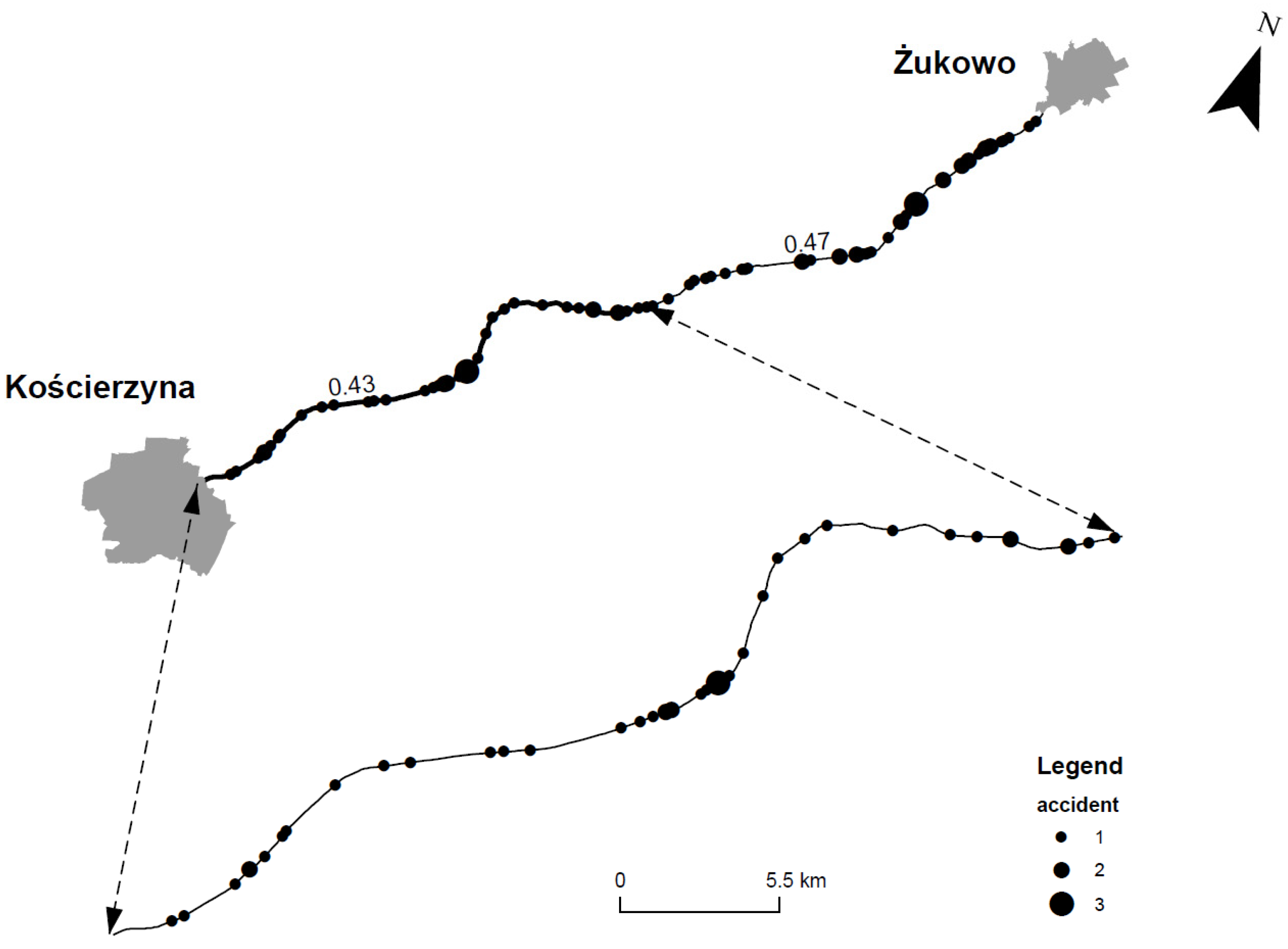
Data recording with the use of a system built for the purposes of this research and verification of the results were carried out on pre-selected road segments. An example of a measured segment is shown in Figure 1.

The selection basis for the segments was road geometry. The first of the selected segments included a long, uninterrupted sequence of horizontal curves. The second one consisted of horizontal curves of varying curvature, clearly separated with straight-line segments.

The research apparatus consisted of two types of sensors. The first group comprised three integrated digital cameras. It was decided to use GoPro HERO3+ Black edition cameras. All of the these worked in the film recording mode. The resolution was set to 1080 p, and the frame rate was 24 fps, and the view angle was set to ultra-wide (full utilization of matrix, without cropping). Moreover, the measuring system included a mobile Global Navigation Satellite System (GNSS) receiver (Leica Viva CS15) with a built-in GSM modem, allowing for access to adjustments made available by Real-Time Network (RTN). This method was selected because the whole area of interest was covered by mobile internet cellular network. During the experiments, adjustments were obtained from the ASG—EUPOS network using Master and Auxiliary Concept (MAC) solution. The positions recorded by the receiver were transmitted in real-time to the portable computer with ArcGIS (Esri) software. This solution provided preliminary verification of the acquired data already during the experiments. In the event of unpredicted disturbances in data recording, the team could simply repeat the experiment. The films acquired during the measurements were computer post-processed. The processing was used to synchronize the film with the time measurement, then, using picture analysis, data regarding the location of the vehicle on the road were obtained. In effect, the offset between the vehicle location and the axis line of the road was obtained. All positions acquired from GPS were adjusted for the calculated offset. Such data preparation minimized errors due to the driving line instability. The final data integration was carried out using ArcGIS (Esri).

The accumulated data was re-checked for correctness. The checks covered both the horizontal coordinates data and any recording errors in the data. This was accomplished by checking whether the recorded points plotted on the actual orthophotomap of the investigated road were consistent with its outline or plotted outside of it. The methodological procedures were performed in order to eliminate the effects of extreme values on the results, possibly leading to erroneous conclusions. The next step in the analysis was to check whether the error for the recorded point fell in the 0.0050 m to 0.012 m interval.

The data was then selected and grouped. Points were verified in terms of relative proximity. First, points with neighboring points at the distance of the assumed minimum tolerance, e.g., 1 m, were identified. This is a necessary condition for further analysis, and the proximity arises from locations where the vehicle speed was reduced to 0 km/h. The next check was related to interruptions in measurement taking, resulting from the horizon being obscured by thick vegetation, trees, or high-rise buildings. A longer interruption in the position recording would increase distances between subsequently recorded points. In the case of distances larger than the maximum tolerance of 100 m, points were treated as belonging to separate measurement sequences. Only points belonging to the same sequence were analyzed as a whole in further parts of the algorithm.

3. Theory and Calculation

A non-urban road may be treated as a continuous line and divided into closed and limited segments. According to the Stone–Weierstrass theorem, these segments may be described with a polynomial. In our case, this means that the shape of the actual road within the single segment could be described with a certain analytical function and with any level of accuracy. From field measurements, we had a finite set of points located on the investigated road. As assumed earlier, these points should belong to the curve that describes the road. This formulation of the problem reduces it to the problem that has been solved many times before, i.e., finding the best fit curve.

The correct solution of the approximation problem calls for defining the family of the approximation functions. The team assumed that within a single segment [a,b], the road could be described as a straight line or a section of a circle. In order to define the borders of the curves, relations between three subsequent points $P_i\left(x_i,y_i\right)$; $P_{i+1}\left(x_{i+1},y_{i+1}\right)$; $P_{i+2}\left(x_{i+2},y_{i+2}\right)$ located along the road axis were considered. If in a given location the road was straight (no curves), the points should belong to the same straight line, thus they were described by the function ${\psi }_m^l\left(x\right)$ (where m denotes function identifier, e.g., 1, 2, 3…), in our case, the polynomial $\left(1\right)$. It was assumed that in order to differentiate the functions which describe road segments as straight lines, the marker ${\psi }_m^l$ would be added, and for road sections classified as curves, marker ${\psi }_m^o$ was added. The conditions of collinearity of the three points may be expressed with two straight-line equations (Equation (1)), which will represent the same straight line if all the coefficients are identical.

$$\{\begin{array}{l}{\psi }_1^l:0=\left(x_{i+1}-x_i\right)y+\left(y_i-y_{i+1}\right)x-y_i{x}_{i+1}+y_{i+1}{x}_i\hfill \\ {\psi }_2^l:0=\left(x_{i+2}-x_{i+1}\right)y+\left(y_{i+1}-y_{i+2}\right)x-y_{i+1}{x}_{i+2}+y_{i+2}{x}_{i+1}\hfill \end{array}$$

(1)

For the purposes of further considerations, the differences of the subsequent coefficients of simple equations were marked as E₁, E₂, and E₃ (Equation (2)).

$$\begin{array}{l}{E}_1=\left(x_i+x_{i+2}\right)y_{i+1}-\left(y_i+y_{i+2}\right)x_2=0\hfill \\ E_2=y_i-2y_{i+1}+y_{i+2}=0\hfill \\ E_3=x_i-2x_{i+1}+x_{i+2}=0\hfill \end{array}$$

(2)

The above relationships could be used to assign each recorded point of the road to either a straight line or to a section of a circle. The calculations answer the question as to whether a given curve connects to another curve or to a straight section.

It must be noted that the condition of collinearity of the points is not strictly met even on a straight-lined segment of the road. This is due to the finite level of accuracy with which the position of each subsequent measuring point was identified. However, this issue could be resolved by making the condition less rigorous. Based on known uncertainties in defining the positions of the points, using a complete differential, maximum uncertainty for expressions E₁, E₂, and E₃ were calculated (Equation (3)). With the above assumptions, we reformulate the necessary condition for the existence of a curve, which can be expressed as

$$\{\begin{array}{c}\left|\left(x_1+x_3\right)y_2-\left(y_1+y_3\right)x_2\right|>\Delta E_1\\ \left|y_1-2y_2+y_3\right|>\Delta E_2\\ \left|x_1-2x_2+x_3\right|>\Delta E_3\end{array}$$

(3)

where ΔE₁, ΔE₂, and ΔE₃ denote the maximum uncertainties for expressions E₁, E₂, and E₃.

On the basis of the points allocated to a straight line, we could calculate the parameters of the straight line with approximation, using the straight-line equation as a polynomial (Equation (4)).

$$f_1\left(x\right)=a_0+a_{1}x=y\left(x\right)$$

(4)

The function ${\psi }_m^l\left(a_0, a_1\right)$ for points $\left\{\left(x_i,y_i\right)\left[i=1,2\dots n\right]\right\}$ is consistent with the format of Equation (5),

$${\psi }_m^l\left(a_0, a_1\right)={\displaystyle \sum }_{i=1}^n{\left(y_i-a_0-a_1{x}_i\right)}^2$$

(5)

where n denotes the number of points of the considered road segment.

By solving the system of Equations (6) and (7), we receive formulas for the coefficients which define a straight line describing a given road segment (Equation (8)):

$$\frac{\partial {\psi }_m^l\left(a_0,a_1\right)}{\partial a_0}=2{\displaystyle \sum }_{i=1}^n\left(y_i-a_0-a_1{x}_i\right)\left(-1\right)=0$$

(6)

$$\frac{\partial {\psi }_m^l\left(a_0,a_1\right)}{\partial a_1}=2{\displaystyle \sum }_{i=1}^n\left(y_i-a_0-a_1{x}_i\right)\left(-x_i\right)=0$$

(7)

$$a_1=\frac{n{{\displaystyle \sum }}_{i=1}^n{x}_i{y}_i-{{\displaystyle \sum }}_{i=1}^n{x}_i}{n{{\displaystyle \sum }}_{i=1}^n{x}_i^2-{\left({{\displaystyle \sum }}_{i=1}^n{x}_i\right)}^2}; a_0=\frac{{{\displaystyle \sum }}_{i=1}^n{y}_i{{\displaystyle \sum }}_{i=1}^n{x}_i^2-{{\displaystyle \sum }}_{i=1}^n{x}_i{{\displaystyle \sum }}_{i=1}^n{x}_i{y}_i}{n{{\displaystyle \sum }}_{i=1}^n{x}_i^2-{\left({{\displaystyle \sum }}_{i=1}^n{x}_i\right)}^2}$$

(8)

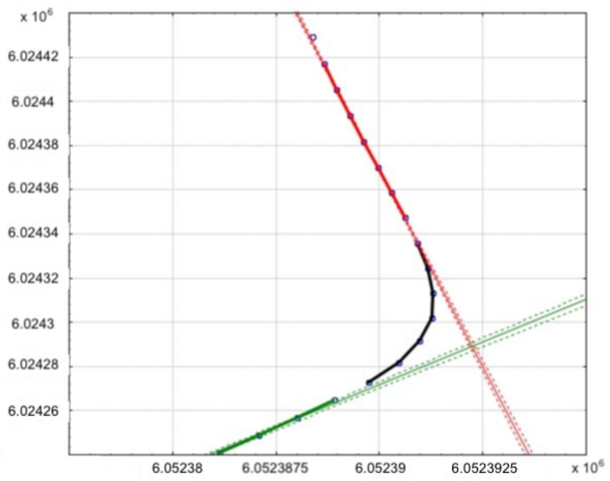
Determining straight-line segments of the road as functions makes it possible to determine the angle at which the roads would cross. For example, the functions which describe line l₁ (red on the graph) and l₂ (green on the graph) which could be seen in Figure 2, could be described with functions (Equation (9)):

$${\psi }_1^l=3.5043\times {10}^7-4.4481·x;{\psi }_2^l=-2.7039\times {10}^5+0.9649·x;$$

(9)

Based on the points classified as being part of a curve, we can approximate a curve. The processed data was used to determine such parameters as the center of the circle, the radius, and the curve length. Beginning with a circle equation in its canonical form (Equation (10)), it could be transformed into to the format of Equation (11).

$${\left(x-a\right)}^2+{\left(y-b\right)}^2=r^2$$

(10)

$$y^2+x^2+a^2+b^2-r^2-2ax-2by=0$$

(11)

We introduce new variables a₀, a₁, a₂ (consistent with Equation (12)). These transformations turn the circle equation into a second-degree polynomial (Equation (13)):

$$a_0=a^2+b^2-r^2; a_1=-2a; a_2=-2b$$

(12)

$$f_2\left(x\right)=a_0+a_{1}x+a_{2}y+y^2+x^2=y\left(x\right)$$

(13)

The function ${\psi }_m^o\left(a_0, a_1, a_2\right)$ for the points $\left\{\left(x_i,y_i\right)\left[i=1,2\dots n\right]\right\}$ takes on the format of Equation (14). Using the approximation of a square function, we can solve equation system (15)

$${\psi }_m^o\left(a_0, a_1, a_2\right)={\displaystyle \sum }_{i=1}^n{\left(a_0+a_{1}x+a_{2}y+y^2+x^2\right)}^2$$

(14)

$$\{\begin{array}{l}\frac{\partial {\psi }_m^o\left(a_0, a_1, a_2\right)}{\partial a_0}=2{\displaystyle \sum }\left(y^2+x^2+a_0+a_{1}x+a_{2}y\right)·\left(1\right)=0\\ \frac{\partial {\psi }_m^o\left(a_0, a_1, a_2\right)}{\partial a_1}=2{\displaystyle \sum }\left(y^2+x^2+a_0+a_{1}x+a_{2}y\right)·\left(x\right)=0\\ \frac{\partial {\psi }_m^o\left(a_0, a_1, a_2\right)}{\partial a_2}=2{\displaystyle \sum }\left(y^2+x^2+a_0+a_{1}x+a_{2}y\right)·\left(y\right)=0\end{array}$$

(15)

By implementing mathematical consideration through script-creation, we obtained descriptions of all the road segments (one curve with two straight-line segments). The sample scripts can be found in the supplement to this paper. These tools could be used to determine the parameters of road curves.

4. Results

The methods described above were used to obtain valuable information about road geometry. Sample data for the surveyed road section could be found in

Table 1. Data characterizing segments of road curves.

Objected	Circle Diamete [m]	Length of Curve [m]	Beginning of Curve [m]	Middle of Curve [m]	End of Curve [m]
40	801.42	124.49	288,853.56	288,915.81	288,978.06
46	256.31	99.27	285,797.75	285,847.39	285,897.02
48	895.37	157.25	285,503.81	285,582.43	285,661.05
56	471.05	170.11	281,647.82	281,732.87	281,817.92
60	509.93	167.99	280,894.10	280,978.09	281,062.08
62	550.03	189.95	280,483.19	280,578.16	280,673.14
63	181.14	89.18	280,381.84	280,426.44	280,471.03
66	622.82	100.68	280,076.36	280,126.71	280,177.05
68	271.47	216.05	279,704.29	279,812.32	279,920.35
70	888.12	104.33	279,562.34	279,614.49	279,666.66
78	162.05	91.12	277,357.82	277,403.37	277,448.93
80	423.91	164.48	277,064.02	277,146.26	277,228.50
82	393.77	97.34	276,200.00	276,248.67	276,297.34
84	121.67	26.11	275,921.27	275,934.33	275,947.39
86	610.66	133.62	274,109.48	274,176.29	274,243.11
88	392.09	176.43	271,277.14	271,365.36	271,453.57
94	914.79	126.69	269,862.06	269,925.41	269,988.76
96	1648.89	175.97	269,208.75	269,296.74	269,384.72
98	754.86	159.12	269,036.61	269,116.18	269,195.74
100	394.50	113.36	268,666.87	268,723.55	268,780.23
108	535.59	251.16	266,850.73	266,976.31	267,101.89
110	419.80	154.17	265,571.92	265,649.01	265,726.10
112	731.21	173.12	265,269.80	265,356.36	265,442.92
114	304.73	103.93	264,963.62	265,015.58	265,067.55

.

The principle for obtaining road curve parameters in the sample fragment is shown in Figure 3.

Based on the experiments acquired during the tests, the research team decided that one more stage in the data processing was needed. The two-stage algorithm failed to provide an optimum classification for the points located at the curve limits, as it did not assign them clearly to either the curve or to a straight-line. The maximum curve fitting error at this stage was 4 m; hence, the second stage was introduced to reduce this error, and thus, unambiguously assign a point to either the curve or the straight line. A generally better fit could have been achieved if some extreme points had been allocated to the straight-line, rather than to the circle. In order to eliminate this point classification error at the curve extremities, a third level of data analysis was introduced to provide the best assignment of points to either a straight line or to a curve. Previous research resulted in the assignment of points to a straight-line or a curve in a local approach—3 subsequent points were considered. On the basis of the determined point classification, a further section of the algorithm checked subsequent segments of the curve, determined by the assignment of a curved or straight line. We selected the first group of points which share the same class: according to Figure 4, these are points which are in a straight line P, with the exception of the last point. Whether the point is in the straight line or in the curve is subject to analysis (the point marked with a red circle, Figure 4) and the remaining points were assigned to the curve class L. On the basis of the points classified as straight-line, we calculated the parameters of the straight line using linear approximation. On the basis of the points classified as a curve, we fit in a circle. With the parameters of the circle and the straight line available, we calculated the distance of point n and received the value dp as the distance from point n to the straight line, and dl as the distance of point n from the curve.

If dl > dp, then point n fits the straight line more than the curve to which it was assigned, so point n was reassigned to the straight line. Afterward, the next point in the curve was investigated, the analysis was carried out again, and we calculated new parameters for the straight line and the curve, and tested point n+1. The analysis continued until dp was larger than dl or the curve had the minimum number of points for approximation, which equals 4.

If dl < dp, then the point was correctly assigned to the curve and was not reclassified; instead, the last point of the straight-line was tested. The same procedure was used to test subsequent points of the straight-line until dl was larger than dp or the number of points for straight-line approximation was equal to 3.

5. Discussion

The main purpose of this research was to present and assess IT tools which automate the determination of the geometric parameters of non-urban roads. The assessment of these tools was carried out with the use of real data recorded on roads. The goal was achieved by testing several hypotheses regarding the correlations between geometric road parameters and road safety. This field study covered several segments of non-urban roads with a total length of 152 km. The results presented in this article refer to one selected part of the track which had a length 23 km. The test segment was characterized with a large number of horizontal curves and a high incidence of road collisions. The values in

Table 2. Safety characteristics of the analyzed road section.

Parameter	Value
Length of curve segments [km]	5.758
Length of straight-line segments [km]	18.200
Collisions on curves	24
Collisions on straight-lines	17
Numbers of collisions/1km curve	4.16
Number of collisions/1km straight-line	1.06

demonstrate that collision density on curved segments was four times higher (measured as the number of collisions per km of road) than on straight-line segments.

The collected road data was grouped into those describing curves and straight-line road. The use of functions to describe the various segments of the road proved difficult at the points where curves meet straight lines. In these areas, the recorded points $P_i\left(x_i,y_i\right)$ could be classified to the functions which describe road sections as straight lines ${\psi }^l$ and, at the same time, as curves ${\psi }^o$. A solution to this problem involved a numerical method which was proposed to unambiguously assign each point to one function only. The code of the proposed script could be found in supplementary materials.

As shown in the test results obtained by the team, other factors affect the safety of specific road sections, which are as follows: the number of horizontal curves as a sequence of connected curves, horizontal alignment of the road, the direction of on-curve movement, and the total length of curves. While the first of the factors, i.e., the sequence of connected curves, has been researched previously [9], this was not in the context of the total length of curves. The road characteristics presented in Figure 4 illustrates the strong correlation between the length of a road curve and the accidents on that section. The results suggest that the method was useful and should be developed further. The tool for road safety management described here could be used as one way to automate the procedure.

It should be noted; however, that the accuracy of rural road accident positioning leaves a lot to wish for. Although road police have had accident-positioning equipment in operation for two years, mistakes are still made. Therefore, the road accident database needs verification. If this could be accomplished, the results would show an even greater match between accident locations and curves on the roads. The next step should be to implement the method on the remainder of the road network. The alignment of regional and local roads is a far more serious hazard than that on national roads.

Authors should discuss the results and how they can be interpreted with perspectives of previous studies and working hypotheses. The findings of this study and their implications should be discussed in the broadest possible context. Future research directions may also be highlighted.

6. Conclusions

According to the results of the research carried out by the research team, road safety analyses should include road geometry factors related to horizontal curves. These factors include the number of horizontal curves as a sequence of connected curves, the radiuses of horizontal curves, the direction of travel along the curve, and the total length of the curves. The first of these factors, i.e., a sequence of connected curves, was investigated [9], but not in the context of the length of all curves. The road characteristics presented in Figure 3 illustrate the correlation between the road curve and collisions on a given road segment (accumulation of the number of collisions on horizontal curves). The results presented show that the methodology was useful and needs to be further developed. In the context of the road inspection introduced four years ago to the national road network as one of the road safety management elements, the tool described here could contribute to automating this procedure.

It should be noted that the precision with which collision locations are documented on rural roads today is woefully inadequate. The traffic police have only been equipped with devices that can determine the location of incidents two years ago; however, there are errors in recording incident coordinates. There is a need; therefore, for the verification of the collision database. More precise data can be used to correctly adjust the parameters of horizontal curves to build road safety measures. The next step should be the implementation of the method on the remaining road network. Traffic hazards related to road geometry on regional and local roads have even more serious consequences than on national roads.