Glacier Dynamics in Changme Khangpu Basin, Sikkim Himalaya, India, between 1975 and 2016

1
Department of Geography, North-Eastern Hill University, Shillong, Meghalaya 793022, India
2
Centre for the Study of Regional Development, School of Social Sciences, Jawaharlal Nehru University, New Delhi 110067, India
*
Author to whom correspondence should be addressed.
Geosciences 2019, 9(6), 259; https://doi.org/10.3390/geosciences9060259
Submission received: 2 May 2019
/
Revised: 22 May 2019
/
Accepted: 23 May 2019
/
Published: 10 June 2019
(This article belongs to the Special Issue Cryosphere II)
Abstract
:This study provides a high resolution glacier database in the Changme Khangpu Basin (CKB) using LANDSAT 8 (2014) and Sentinel-2A image (2016), mapping of 81 glaciers that cover a 75.78 ± 1.54 km2 area. Composite maps of land surface temperature, slope and Normalized differential Snow Index have been successfully utilized in delineating near accurate debris cover boundary of glaciers. The cumulative controlling parameters of aspect, elevation, slope, and debris cover have been assessed to evaluate the nature of glacier distribution and dynamics. The local topographic settings seem to have significantly determined the glacier distribution in the CKB. Almost 20% area erstwhile under glacier cover has been lost since 1975 at an average rate of −0.453 ± 0.001 km2a−1. The recent decade (2001–2016) has witnessed a higher rate of area shrinkage (−0.665 ± 0.243 km2a−1), compared to a relatively lower rate of recession (−0.170 ± 0.536 km2a−1) between 1988 and 2001. The lower rates of glacial recession can most likely be induced regionally due to relatively cooler decadal late summer temperatures and peak in the monsoon spell. Glaciers with western and north-western aspects showed more vulnerability to area loss than the rest of the aspects. Lower altitude glaciers have receded faster than ones perched up on higher elevations. The rate of glacier area recession has been nearly twice that on clean glaciers as compared to debris-covered glaciers in the CKB.
1. Introduction
Large variability and oscillation in climate post-industrial revolution has negatively impacted the health of mountain glaciers and their dynamics. These changes have altered the glacier area, volume, length and width, and snout positions, along with changes in other physical properties like debris cover, ice densities, ice velocities, glacier surface appearance, glacier surface temperature, etc. [1]. Tropical and subtropical glaciers have been studied to be more sensitive to such changes [2]. The modern day analysis of these glaciers is significantly crucial as these support the 10 largest river systems in Asia, along with a population of over 1.3 billion [3]. Furthermore, the future runoff from the glacierized catchments can be predicted from the present glacier-climate interaction assessment, essential from any policy-making perspective [4].
Even within the east-west extension of the Himalayas, the distribution and the fluctuation of glaciers are highly variable over time and space [5,6]. Glaciers in Karakoram, part of the Hindu Kush Himalaya (HKH) are relatively stable, and some of these have even exhibited little advance over the last decade [6]. On the contrary, the Khatling glacier in the Garhwal Himalayas is retreating at an alarming rate of 88 ± 0.3 ma−1 [7]. A relative slower rate (0.08 ± 0.07 km2a−1) of glacier recession has however been reported in the Ravi basin of the Himachal Himalayas [8]. Research on the HKH using remote sensing data shows that the Sikkim region reflected maximum glacier retreat, followed by Karakoram and the Himachal Himalayas [5]. Such spatiotemporal variety in glacier recession is probably due to topographic, geologic and climatic interferences [6,9,10,11]. Therefore, it is imperative to assess the topographic and climatic parameters to analyze the distribution and variability of glaciers. Due to the paucity of higher-resolution accurate glacier inventories, the preparation of a neat, accurate higher-resolution glacier database is required. Hence, the assessment of glacier-climate interaction requires repeated creation of the higher resolution glacier inventories and observation of glacier parameters over the temporal and spatial scale. Corona and Declassified Hexagon aerial photograph series have proved to be a robust dataset for glaciological studies [12,13]. There are no published studies on the Changme Khangpu basin (CKB) monitoring of glaciers.
The basin is located on the eastern part of the HKH, the least studied and least understood the region, having extreme topography, coupled with different climate systems. Considering the local level asymmetry in topography, climate and glaciers, the present study provides a near accurate high-resolution glacier database (2016). This study also aims to quantify glacier dynamics since 1975.
2. Regional Setting
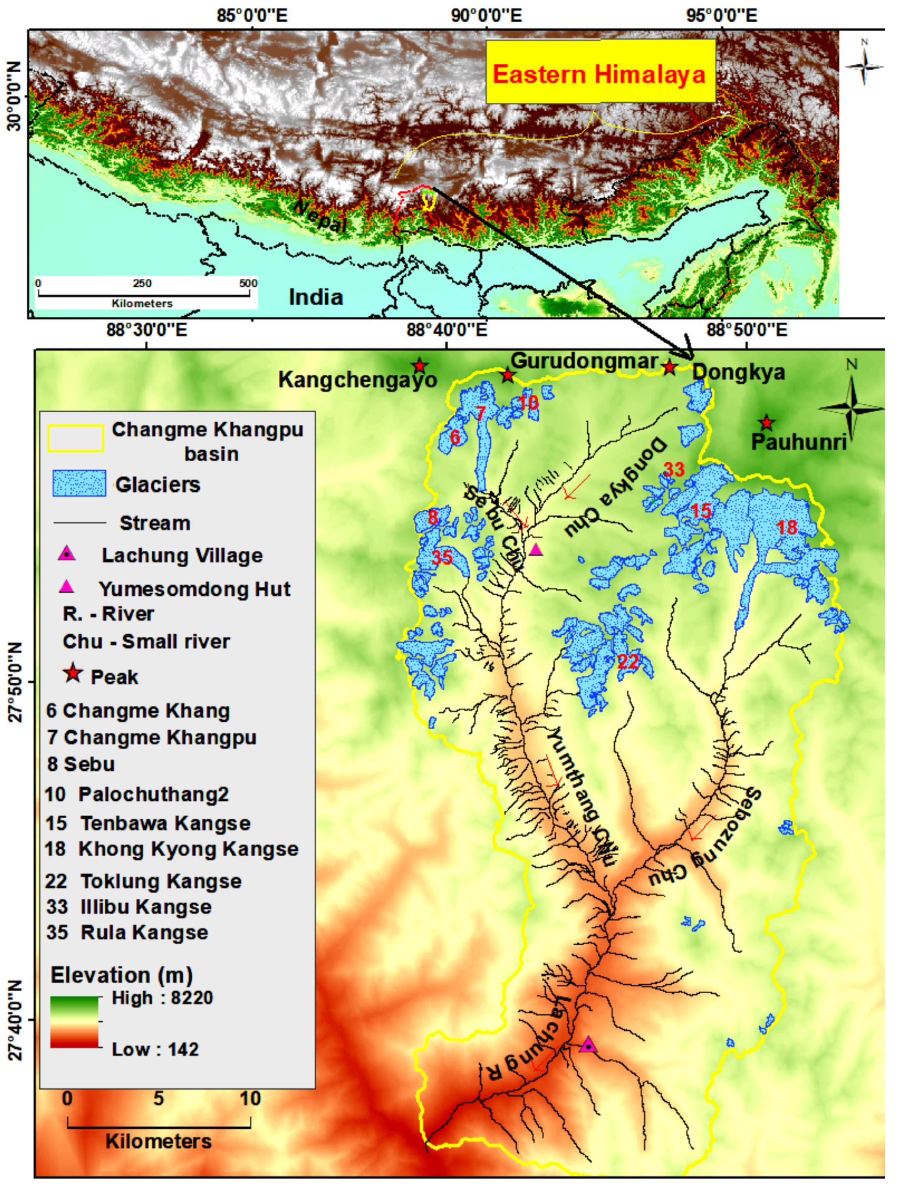
The upper catchment of the Tista river basin, a major tributary of River Brahmaputra, represents Sikkim Himalaya and comprises of a total of 449 glaciers, covering an area of 706 km2, with an estimated ice volume of 39.61 km3 [14]. Out of the five 5th order basins (Supplementary Table S1), the CKB marks the eastern most glacier bearing basins of the Sikkim Himalayas, located between 27°36’15.393” N and 27°59’14.07” N; 88°38’12.805” E and 88°53’13.214” E [14] (Figure 1). Kangchengayo, Yulhekang, Gurudongmar, Dongkya, Pauhunri are the major mountain peaks of Kangchengayo-Pauhunri massif, that demarcate the northern boundary of this basin. The Yumthang Chu and Sebozung Chu confluence at Dombang flows into the Lachung Chu that drains the CKB. The word ’chu’ is the local name for a stream. The Changme Khangpu (CK), Illibu Kangse, and Khonkyong Khangse are some of the major glaciers in this basin.
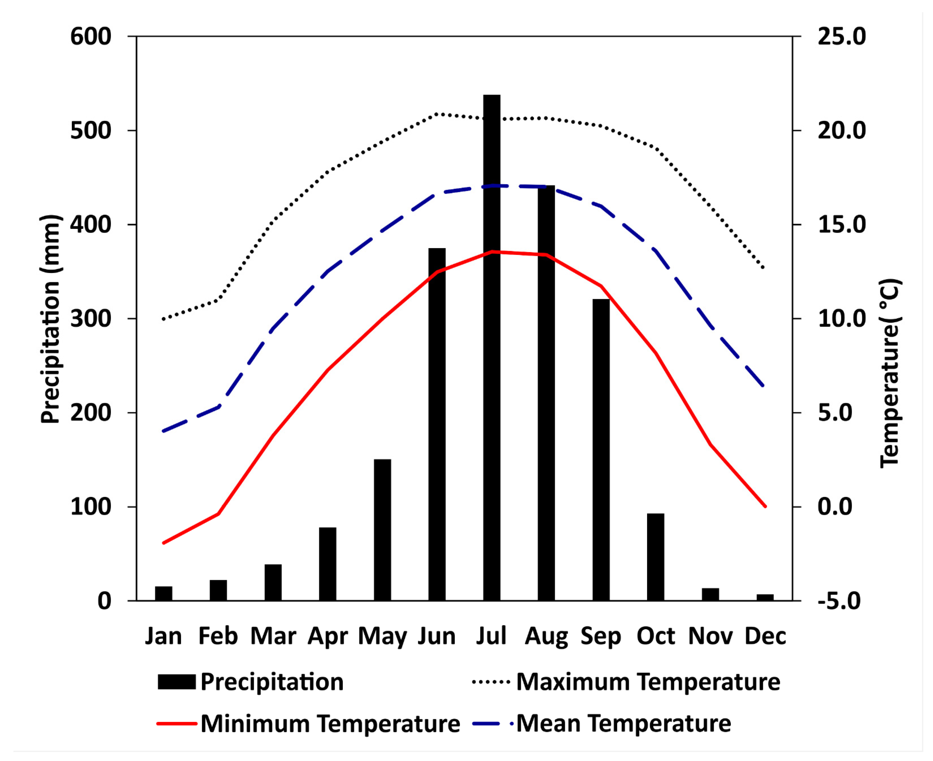
Unlike the glaciers in other parts of the HKH, glaciers of the Eastern Himalayas (EH) are solely the summer accumulation type. The climate is characterized by little precipitation during the winter months, and therefore, are very sensitive to summer precipitation and air temperature [11,15,16,17]. Due to the proximity of Sikkim Himalaya to the Bay of Bengal, the South West monsoon directly provides torrential precipitation in this region. The climograph (Figure 2) (1901–2002) shows that long term average temperatures do not exceed 20 °C, whereas, monthly precipitation varies from 7 mm in December to 538 mm in July. The highest precipitation occurs in the month of July, followed by August (442 mm), and June (375 mm), whereas December and January are consecutively dry months. Debnath et al. [18] have reported that the Kangchengayo-Pauhunri massif experienced a trend of increased atmospheric temperature almost for all of the months except February, April, and May. The CKB lies on the windward side of the Kangchengayo-Pauhunri massif. Mann-Kendall trend analysis of long-term precipitation, average temperatures (1950–2014) and Sen’s slope analysis of the rate of change have furnished a more specific view of climate anomalies in the CKB (Table 1) [19,20]. Monsoon and post-monsoon seasons are observed to be warming (at 0.0001 significance level) at rates of 0.021 °Ca−1 and 0.027 °Ca−1, and the temperature of winter and pre-monsoon seasons are observed to be increasing at the rate of 0.014 °Ca−1 and 0.019 °Ca−1 (at 0.001 and 0.003 significance levels), respectively. Precipitation in the winter and pre-monsoon seasons show increasing trends at a significant level, but monsoon and post-monsoon seasons do not reflect any trend. The winter and pre-monsoon lesser warm temperatures may be attributed to wetter atmospheric conditions in these seasons.
3. Data Source
The specific regional climatic characteristic of the Sikkim Himalayas restricts cloud-free satellite data during the period of pre-monsoon and monsoon seasons. Hence, the minimal cloud coverage images of the post-monsoon months (October to early January) have been analyzed [5,18]. In this study, temporal satellite data of the declassified Hexagon satellite images (KH-9) for the year 1975, Landsat 4 Thematic Mapper (TM) (1988), Landsat 7 Enhanced Thematic Mapper Plus (ETM+) (2001) and Landsat 8 Operational Land Imager and Thermal Infrared Sensor (OLI-TIRS) (2014), Sentinel-2A image (2016) and images on the Google Earth platform were used. Map published by The Swiss Foundation for Alpine Research (1:150,000) of the Sikkim Himalayas (1981) was used for the local level information for major peaks, spots, bench marks, glaciers and glacial lakes in this study area. The KH-9 image, Landsat images, and Shuttle Radar Topography Mission digital elevation model (SRTM DEM) downloaded from the USGS website (http://earthexplorer.usgs.gov), and Sentinel-2A image were been downloaded from the Copernicus Open Access Hub (https://scihub.copernicus.eu/dhus/#/home). The details of the data set used is given in Table 2. The SRTM DEM (30 m) satellite images were analyzed because of its better accuracy. A accuracy assessment of freely available DEM images has been done using the statistical method of lesser root mean square error (RMSE) [18].
Unfortunately, the poor network of meteorological stations persists over the Asian high mountainous region [21]. The scarcity of the instrumental climatic data was overcome using various satellite or average of observational based gridded data [21,22,23]. For this study basin, the monthly gridded (0.5° × 0.5°) precipitation (in mm) and temperature (in °C) data for the period of 1950 to 2014 were extracted from the CRU (Climate Research Unit) website (http://www.cru.uea.ac.uk/data). In addition, monthly climatic data of the North District of Sikkim for the period 1901 to 2002 have been downloaded from the India Water portal (http://www.indiawaterportal.org/met_data/).
4. Methodology
A Multi-criteria technique (MCT) was applied to delineate clean glaciers and debris-covered glaciers, using optical as well as thermal remote sensing data and the DEM derived morphometric parameters.
4.1. Pre-Processing and the Rectification of Satellite Images
The pre-processing was carried in the following manner:
- The first step of the MCT was based on radiometric correction of Landsat sensor images by converting the digital number (DN) values of the bands into a common meaningful physical unit (i.e., top of atmospheric or TOA reflectance) [18]. The algorithm provided by NASA (2009) (https://landsat.gsfc.nasa.gov/wp-content/uploads/2016/08/Landsat7_Handbook.pdf) [24] and (2015) (https://www.greenpolicy360.net/mw/images/Landsat8DataUsersHandbook.pdf) [25] were used for conversion of TM, ETM+ and LANDSAT 8 sensor images respectively. The DN values of Sentinel-2A (MSI) bands were also converted into surface reflectance values that have been further used for the manual digitization of glaciers.
- Panchromatic sharpening (Pan-sharpening) is a technique that combines the high-resolution panchromatic data with medium-resolution multispectral data that create a multispectral image with higher-resolution features. The Pansharpening of 2001 (ETM+) and 2014 (OLI-TIRS) images help in enhancing spatial resolution of multispectral bands (up to 15 m). It was aimed at clear visualization of the glacier termini, glacier boundary, and morphology [8]. The Pan-sharpened bands of LANDSAT series have proved to be a good base map for the rectification of Corona and Hexagon images [8,26].
- The reduction of the distortion pattern towards the edges of the declassified KH-9 images is a necessary requirement of image pre-processing. In this regard, KH-9 images were co-registered with the Pan-sharpened band of LANDSAT 8. The KH-9 images have a complex geometry and large size (2 GB). Therefore, 7 subsets of the KH-9 images for the entire CKB were generated and 150 to 200 common points for each subset were identified in the co-registration process. The co-registration technique of KH-9, given by Padmanabha et al. [27] and Surazakov and Aizen [28], was used. The average horizontal shift between the KH-9 and LANDSAT 8 Pan image amounts to 7.51 m (0.94 pixels). The Sentinel-2A images were co-registered with LANDSAT 8 Pan-sharpened bands, where a 11 m (1.08 pixel) horizontal shift was recorded.
4.2. Mapping Glacier Boundary
4.2.1. Normalized Differential Indexing and Band Ratio
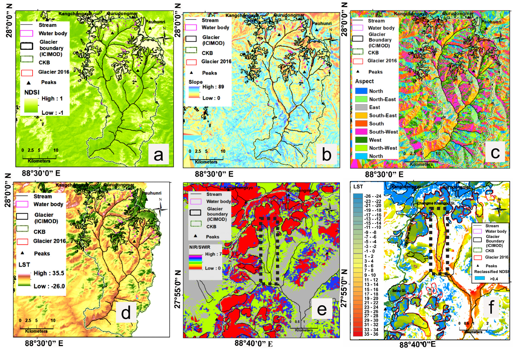
The automated algorithms consisting of various normalized differential indices such as Normalized Differential Snow Index (NDSI), Normalized Differential Water Index (NDWI), and Normalized Differential Vegetation Index (NDVI) were applied to delineate clean glacier ice. The threshold of the NDSI and band rationing are robust and time effective approaches for clean glacier ice mapping [29,30,31] but not for debris-covered [31,32,33]. The present study shows that the given threshold value of NDSI (+0.4 for TM,ETM+ and OLI imagery) coincide with the debris free glacier boundaries but does not match with the debris-covered glacier boundary (Figure 3a). The spectral reflectance value from the ice, which is completely buried under thick supraglacial debris, may not be different from the surrounding non-glaciated areas, and hence NDSI proves to be incompetent in delineating debris covered parts of glacier ice [34]. Snow and glacier ice reflect up to 95% of its incoming solar energy at the visible (VIS) band, but reflects 50–80% at the near-infrared (NIR) region, while rock or debris-covered surface reflectivity is highly varied at visible and near-infrared (VNIR), shortwave infrared (SWIR) and thermal infrared (TIR) regions [35]. The reflectivity and surface temperature of debris cover, varies according to its constituent material [36]. Some researchers have recommended the NIR/SWIR band ratio (using the DN values) to demarcate debris-covered glacier boundaries [34,35]. In our study, Figure 3e represents the NIR/SWIR map which represents a better identification of the debris-covered parts of the glacier. The NIR/SWIR map presents a relatively well defined debris-covered part, as well as clean snow and ice masses of glaciers, but not at a satisfactory level.
4.2.2. Morphometric Parameters
In recent decades, researchers have tried to overcome this problem using morphometric parameters along with thermal information [37,38]. The morphometric parameters comprise the contour pattern, slope gradient, curvature, aspect, break in slope, initiation of streams, emergence of proglacial ponds, etc., derived from the SRTM DEM. The upper limit of the glacier boundary goes up to a 45° gradient in many cases, which have been identified from the reclassified slope map of the CKB (Figure 3b). This reclassified slope map highlights the glacier terminal landforms like laterofrontal moraines. The computed aspect map (Figure 3c) has been used to demarcate the glacier divide.
4.2.3. Land Surface Temperature Measurement
Finally, the land surface temperature (LST) map (Figure 3d) was prepared from the thermal bands of Landsat imageries (2001, 2014). The DN value of LANDSAT images has been converted into top of atmospheric (TOA) radiance to calculate the at-satellite brightness temperature [25]. The USGS [25] provided methodology was been applied for achieving this result. The at-satellite brightness temperature was converted into LST with the help of land surface emissivity (LSE). The LSE was calculated from the assigned threshold value of NDVI that has been performed by previous researchers [39,40,41]. Finally, the LST of the area owing a <15° slope, was masked out. It was observed that the composite map of LST and slope efficiently differentiated the debris-covered part of a glacier (Figure 3f). Therefore, it has been found that the LST, slope and NDSI maps, cumulatively, help to delineate the debris-covered glacier boundaries with comparative ease. It is necessary that the threshold value in each case is chosen carefully. Near the frontal part of CK, the LST reaches around 9 °C (at 4820 m altitude), but decreases to below 0 °C at the altitude of 5250 masl.
4.2.4. Glacier Boundary Delineation and Inventory Map
Manual digitization of the glacier boundary was performed using Sentinel-2A satellite image, Pan-sharpened OLI image (2014) and the satellite images on the Google Earth platform. The outcrops within the glacier mass were delineated and excluded from the glacier area. The smaller than 0.02 km2 isolated ice patches were excluded for the glacier body delineation [8]. The Global Land Ice Measurements from Space (GLIMS) guidelines (http://www.glims.org/MapsAndDocs/guides.html) were followed to define glacier boundaries and classify glaciers. Rock glaciers (RG) are excluded from the glacier inventory [8], although, several rock glaciers exist in the study region. RG in this basin have been identified through the set of criterion mentioned earlier by Whalley and Azizi [42], Chand and Sharma [8]. The topographic influence and significance on the glacier distribution were analyzed through statistical methods. Uncertainty of the mapping was carried out for a higher-resolution glacier inventory, as given by Granshaw and Fountain [43]; Bolch et al. [44,45]. This study recorded 2.0%, 3.6%, 7.1% and 1.9% mapping uncertainty for the images of Sentinel-2 (2016), Landsat ETM+ (2001), Landsat TM (1988) and KH-9 Hexagon (1975), respectively. This multi criterion approach is the utmost important element for accurate boundary delineation of clean and debris-covered glaciers. The monochromatic shades, shadow effect, etc., parameters have been applied to delineate the glacier boundary for the 1975 image from the KH-9 images.
4.3. Temporal Changes
A temporal study of glaciers was carried out for the years of 1975, 1988, 2001, and 2016. For year 2001, due to cloud coverage on some part of the study area, few glaciers could not be delineated to perfection. Therefore, such glaciers were excluded from the study for temporal variation. The uncertainties associated with glacier area changes (EAC) was calculated using the following formula [46]:
where EAC denotes glacier area changes; EA1 and EA2 are the uncertainties associated with the glaciers area of two different periods that are being compared. The snout position change detection was done only for the Changme Khangpu (CK) glacier, (bench mark glacier).
4.4. Field Measurements and Validation of the Mapping
The prepared map, including glaciers and associated landforms derived from satellite data of 2016 has been rectified in the field during the field surveys. Field surveys were carried during the pre-monsoon (i.e., in the month of May) and the post-monsoon period (i.e., in the months of October, November) from 2015 to 2017. The benchmark glaciers and associated surrounding morphology were verified in the field with hand-held GPS.
4.5. Statistical Methods
Shapiro-Wilk distribution test statistics and Q-Q plots were employed to identify the nature of data, i.e., whether the data falls under Gaussian distribution or not. Kendall’s tau_b correlation was used as a non-parametric method to analyze the data. To establish a relationship between the categorical variables (e.g., aspect, frequency and glacial area), box-whisker plots were prepared (Figures 4a, 6a and 8a,b).
5. Result and Discussion
5.1. Regional Distribution of Glaciers in the CKB
This study generated an improved, up to date and comprehensive glacier inventory for the CKB (Supplementary Table S2). The present study would be an important input for the glaciological study of the Eastern Himalayas. In the CKB, a total of 81 glaciers existed in 2016, covering an area of 75.78 ±1.54 km2. Glacier size in this basin ranges from 0.02 to 13.8 km2 (Figure 4a). The distribution of glaciers in the CKB do not fit into a Gaussian distribution (Figure 4a–c) (Table 3) due to high skewness value and high standard deviation (SD). The median size of glaciers is much smaller (0.31 km2), indicating a dominance of small-sized glaciers (Figure 4a). The mean size (0.95 km2) is also comparatively much smaller than many other basins such as, the Upper Ganga (1.06 km2), Chenab (1.15 km2), Beas (1.08 km2), Zemu (1.24 km2), Talung basin (1.54 km2), and Shyok (1.4 km2) [8,9,33]. The observed total glacierised area, as well as the total number of glaciers in this study (2016) were much different from the glacier inventory data from the International Centre for Integrated Mountain Development (ICIMOD) (2011) (92 glaciers covering a surface area of 81.32 km2). Figure 5 indicates a set of small glaciers that have been delineated by ICIMOD (2011), but was not present in the 2001 LANDSAT image.
5.2. The Controlling Topographic Parameters
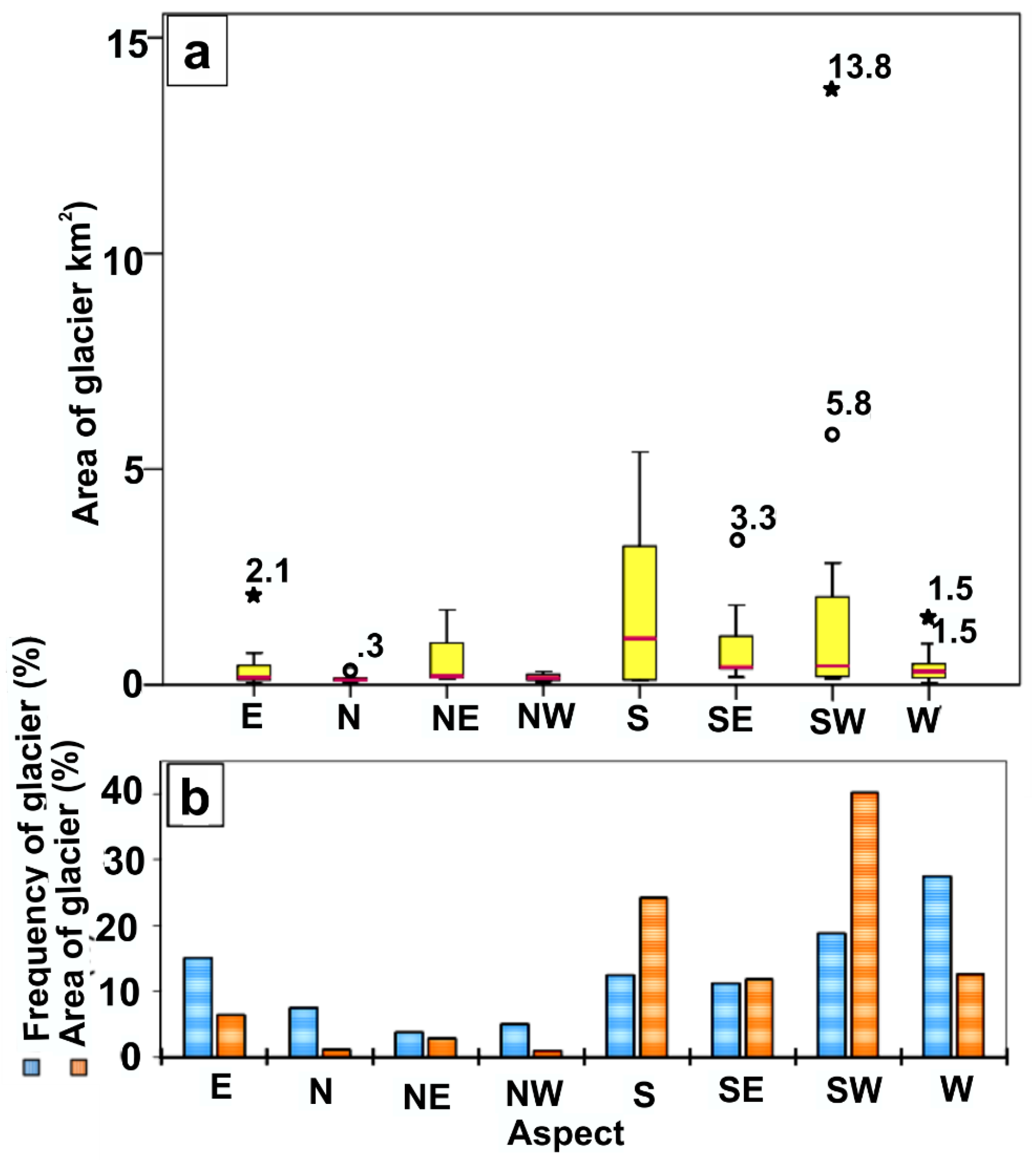
Previous studies have identified numerous climatic and non-climatic parameters such as temperature, precipitation, glacier area, slope, aspect, shape, hypsometry, elevation, etc. as the controlling factors of glacier distribution on the Third Pole region [47,48]. This study shows the large-sized glaciers have mostly south, south-east, and south-west aspect (Figure 4a and Figure 6a). Figure 6a,b shows not only the larger glaciers but also higher frequency and maximum glacial area that are distributed on the aspects mentioned above. Nearly 43% of glaciers are situated on the southern aspect, occupying about 73% of the total glacier area. On the contrary, most of the small-sized glaciers are situated on the eastern, northern, north-eastern, and north-western aspect. The niche glacier, in the study area, is presented as Figure 7a–c. This group of niche glacier is very small in size (0.18 km2 and 0.13 km2), and having a steep slope (average slope is 30°) and on the northern aspect. The field photograph (Figure 7c) presents a fresh talus cone that has descended from the snout of niche-1, and the toe of the talus cone has been truncated by the stream Sebu Chu.
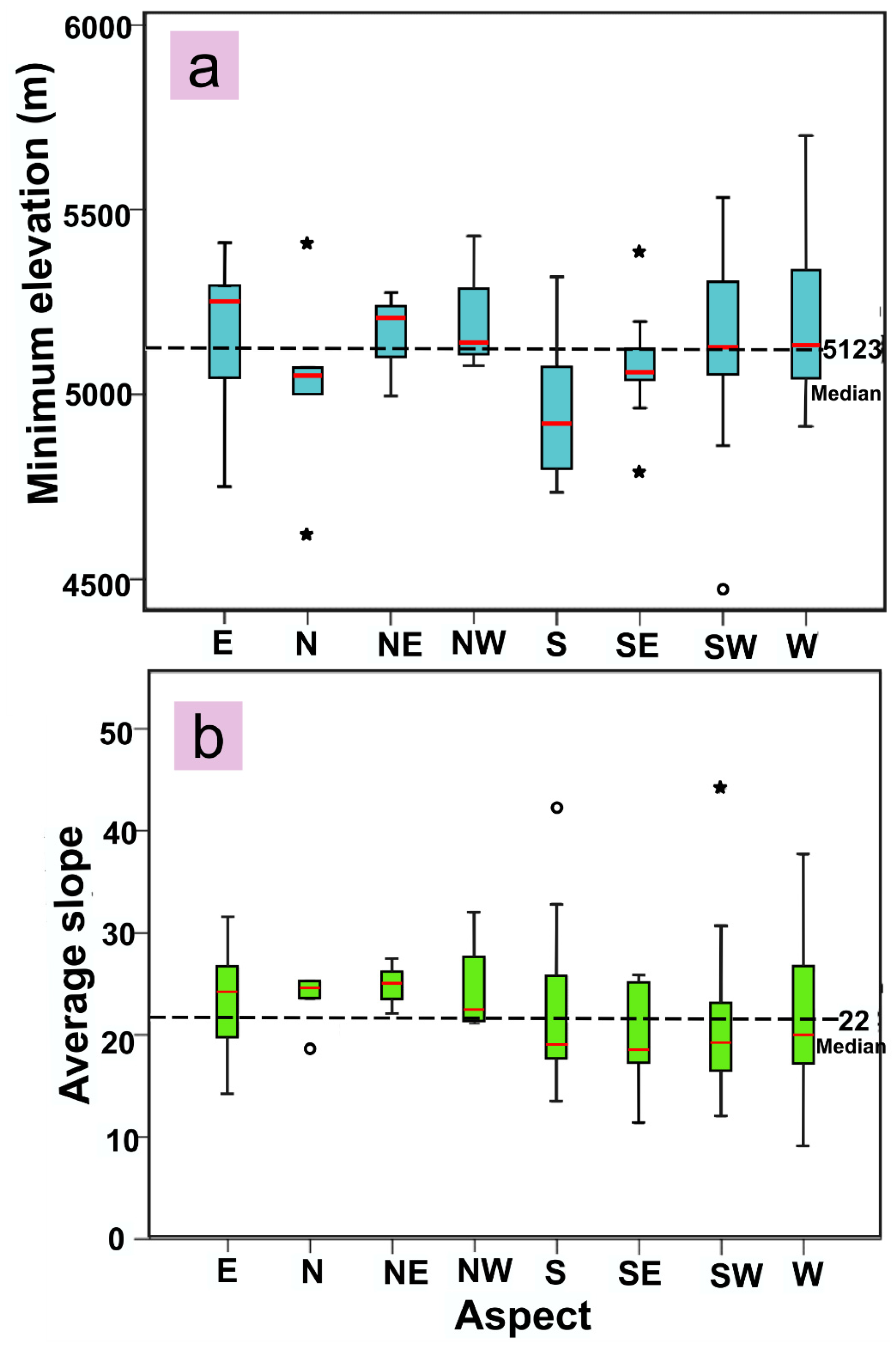
Glacier termini, situated at a lower elevations are more vulnerable to climate change, therefore, the minimum altitude of glaciers become an essential parameter to investigate [8]. In the CKB, glaciers’ termini on southern, south-eastern and northern aspects are situated at the lower altitude (<5100 m) as compared to the other aspects (Figure 8a). Glaciers’ termini on the southern aspect, are situated at the lowest elevation (<5000 m), probably due to the existence of large-sized glaciers on this aspect. The moderate negative relationship (significant at 0.05 level) exists between glacier size, and the minimum elevation occupied by the glacier (Supplementary Table S3). This relationship signifies that the bigger glaciers generally attain relatively lower altitudes.
The most crucial topographic parameter is the slope. Glaciers, here, are distributed on an average slope ranging from 9° to 44°. A significant (at 0.01 level) negative correlation (−0.323) between glacier size and average slope (Supplementary Table S4) also suggests larger glaciers possess a gentle slope and smaller glaciers have a steeper slope (Figure 8b). Glaciers distributed on the southern, south-eastern, south-western and western aspect have gentle slopes (less than 20°). This study reveals that the glacier size in the CKB is determined by the local topographic parameters such as average slope, aspect and altitude.
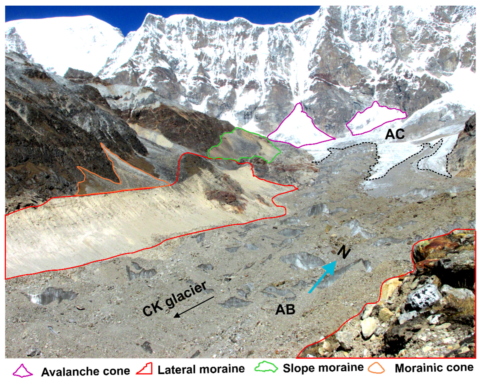
Previous studies had postulated a relationship between surface slope, supraglacial debris cover, and aspects [49]. In the CKB, the maximum proportion (87.6%) of the glaciers are debris free and only 12.1% are debris-covered, yet the average size of these debris-covered glaciers are many times larger than the clean glaciers (Figure 9a,b). The proportion of debris-covered glaciers in the CKB is similar to the basins of North-Western Himalayas, e.g., Jhelum (12%), and Yamuna (18%). The biggest debris-covered glaciers are Khong Kyong Kangse (13.79 ± 0.19 km2), followed by Tenbawa Kangse (5.81 ± 0.11 km2), CK (4.94 ± 0.11 km2), and Rula Kangse (3.35 ± 0.06 km2). About 48% area of the CK glacier is under supraglacial debris cover (Figure 10).
Besides, a considerable number (11) of RG exist in the CKB. The two RG, in the study area, have been represented in Figure 11a,b. Both of them extend to the western direction. The RG-1 is formed on the gentle floor and most probably evolved from a palaeo non-active debris-covered glacier (Figure 11a). Figure 10 exhibits the fresh scree extending downslope from the termini of RG-1. A thermokarst pond has formed between the front of Illibu Kangse glacier and RG-1 (Figure 11c).
The SW monsoon winds provide precipitation at the southern aspect of the mountain; therefore, the glaciers lying on the windward side are directly fed by the same. It appears the interplay between the SW monsoon and southern aspect provides the most favorable condition for the formation of large-sized glaciers and expansion of termini at lower altitudes. Being on the leeward side, the northern, north-western and north-eastern aspects receive relatively less direct-precipitation, and therefore, these higher altitude glaciers possess restricted sizes. Thus, this study reveals that the nature of glacier distribution in the CKB has a profound control of topo-climatic interplay.
5.3. Overall Glacial Area Dynamics in the CKB
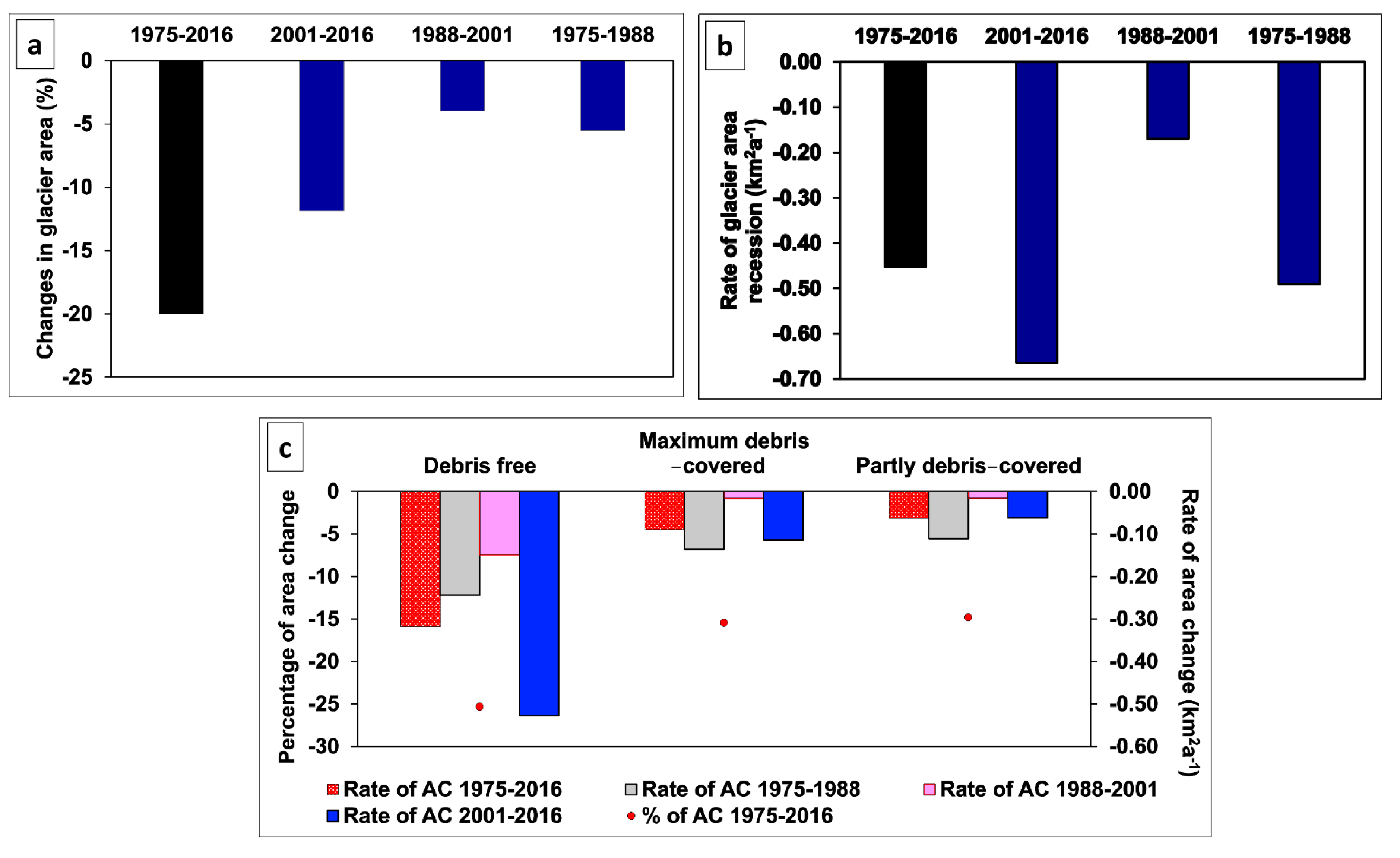
The glacier area dynamic analysis was carried out for 79 glaciers, having an area of 0.02 km2 or more. Here, a 20% glacier area (−18.56 ± 2.61 km2) was lost since 1975 (Figure 12a) (Supplementary Table S5). The overall glacier recession rate in 42 years was recorded at −0.453 ± 0.001 km2·a−1 (−0.507 ± 0.001%), although, decadal variability was observed (Table 4). The annual rate of deglaciation was lower between years 1988 and 2001 (−0.170 ± 0.536 km2·a−1) compared to the previous decade (1975–1988). However, this rate took pace (−0.665 ± 0.243 km2·a−1) during the recent period (2001–2016), but the glacier studies in the Ravi and Chenab basin (NW Himalaya) indicated a decline in the rate of retreat during the past decade (2001–2013) [8,50].
The decadal glacier variability in the CKB somewhat coincides with the decadal late-summer (July, August, and September, i.e., JAS) temperature variability [51,52]. The late-summer temperature at decadal level was reconstructed by Bhattacharyya & Chaudhary [51] and Yadava et al. [52] for the North Sikkim Himalayas based on dendrochronology. Bhattacharyya & Chaudhary [51] recorded that 1978–1987 was the warmest (+0.25 °C) decade at Yumthang (middle part of the CK basin), followed by cooler years in the early 1990s. In addition, Yadava et al. [52] have reconstructed decadal scale warming and cooling periods in Lachung (in the CK Basin) and Lachen since 1852, and reported that the decade 1996–2005 as the warmest period. Borgaonkar et al. [53] found that the Sub-Himalayan West Bengal and Sikkim monsoon rainfall curve attained its peak in the 1990s.
Therefore, it has been summarized that the warmer 1978–1987 decade perhaps accelerated ice melting and hence, a higher rate of deglaciation was observed for 1975–1988. The comparatively cooler late-summer temperature and accelerated monsoon rainfall in the following decade (1990s) may have reduced the ice melting and resulting in the declining rate of deglaciation between 1988 and 2001. Again, the warmest JAS temperature of 1996 to 2005 could have been responsible factor in the rapid pace of area loss (2001–2016) in CKB, not negating the response time influence in glacier studies.
Glacier dynamics are a function of the amount of ablation and accumulation of glacier ice that is controlled by local topo-climatic parameters [50,54]. Here, the regional climatic amelioration was proved to be a determinant factor in the nature of glacial recession. The annual rate of deglaciation (−0.507 ± 0.001%) in the CKB is different from the Ladakh Himalayas (−0.4%), the Garhwal Himalayas (−0.12 to −0.07%), and the Bhutan Himalayas (−0.3%) [55]. Our study points toward the unique nature of the decadal rate of deglaciation in the CKB, as compared to other regions of the HKH. In addition, the topographic parameters have also been assessed in the following sections.
5.4. Role of Topography on Glacial Area Dynamics
5.4.1. Glacier Size as a Controlling Parameter
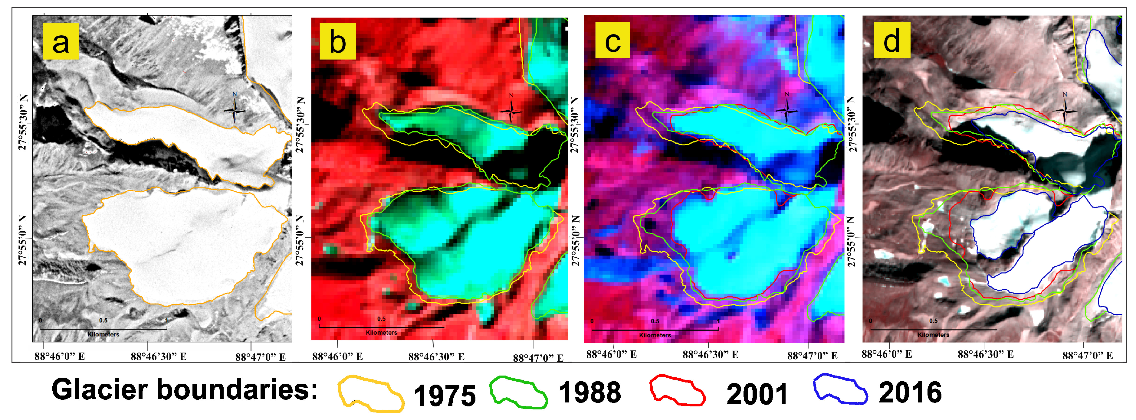
Glacial areas are interrelated with volume or mass which is directly proportional to the changing climate [50,56]. In the CKB, 10% of glaciers have disappeared since 1975, which constitutes about 1.52% of the total glacierised area. The very small-sized glaciers, i.e., cirque and niche (average size is 0.18 km2) disappeared during this study period. In the CKB, a negative correlation (-0.58) between glaciers’ size and area loss (significant at 0.05 level) (Supplementary Table S6) signify a faster response of the smaller glaciers subjected to climate change than larger ones. The bigger glaciers Khongkyong Kangse, Tenbawa Kangse, and CK have lost 11%, 12% and 15% of the total area, respectively. About 6% of glaciers have emerged as a result of the fragmentation from the main glacier since 1975 (Figure 13).
5.4.2. Impact of Debris Cover on Glacial Ice Loss
Debris have a significant influence on the glacier response to climate change [57,58]. This study also reports that the area loss from the debris free glaciers is nearly twice (−0.618% a−1) than debris-covered glaciers (−0.376% a−1 for the maximum debris-covered glacier, −0.361% a−1 for the partially debris-covered glaciers) (Table 5) (Figure 12). It might be due to glaciers with supraglacial debris-covered ablation areas respond differently to climate change than debris free glaciers [57], (2) 5 small-sized debris free niche and cirque glaciers have disappeared during the 42 years’ from this basin.
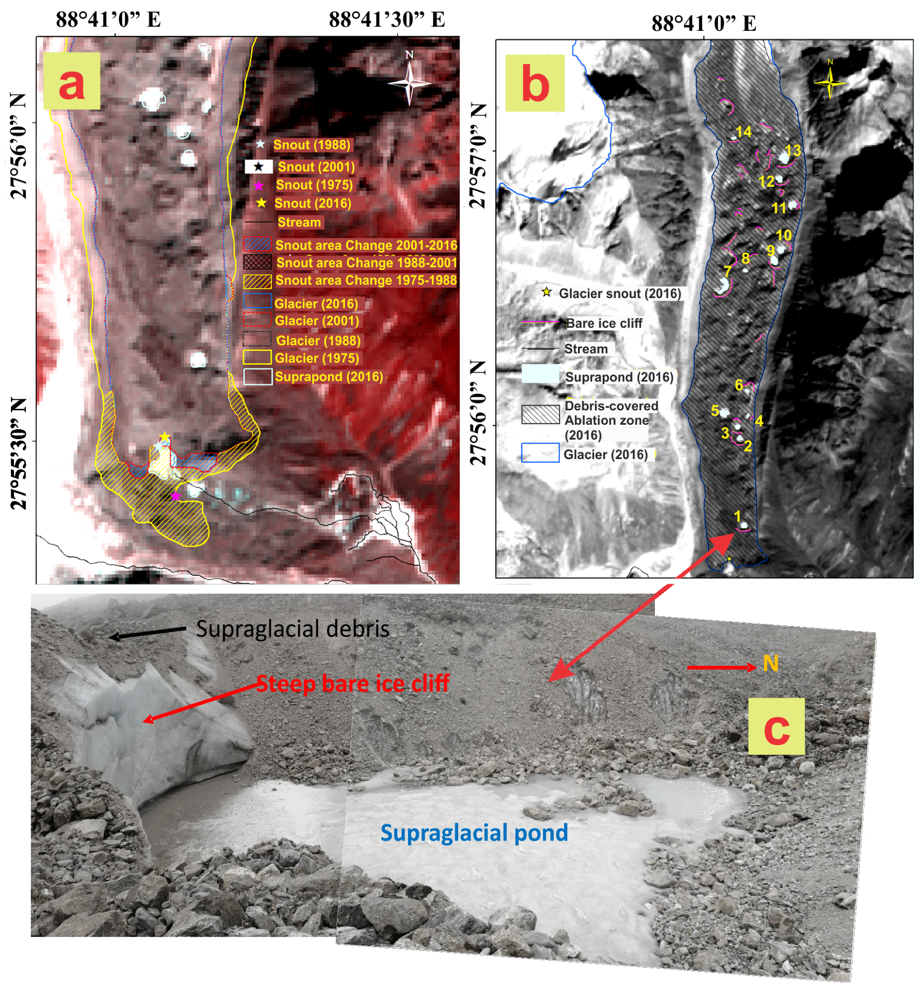
Figure 14a exhibits the snout position of the CK glacier which has receded by 175 m since 1975 at the rate of −4.4 ma−1. Although, the snout position remained stagnant between 1988 and 2016. Therefore, it has been found that the snout of CK glacier retreated at a slower rate than the glaciers of the Western Himalayas. This result might be a consequence of an interplay between glacier ice melting and supraglacial debris thickness, because thick debris often acts as a heat insulator on the ice and hence less glacier ice melting and less snout dynamics [58].
One of the essential components of the ablation budget for the debris-covered glaciers are supraglacial ponds, which act as great mediums of water storage and energy transfer [59]. The thinning of debris-covered glaciers are accelerated mainly with the development of supraglacial ponds [16]. The surface of the supraglacial ponds can absorb seven times greater heat than the average heat absorption of supraglacial debris and the combined effect of this supra-pond, and ice cliffs play a role factor in debris-covered glacier thinning [60]. A total of 14 identifiable supraglacial ponds on the CK glacier have developed since 2001, and were visited during 2016 field season (Figure 14b,c).
5.4.3. Aspect and Altitude as the Controlling Factors
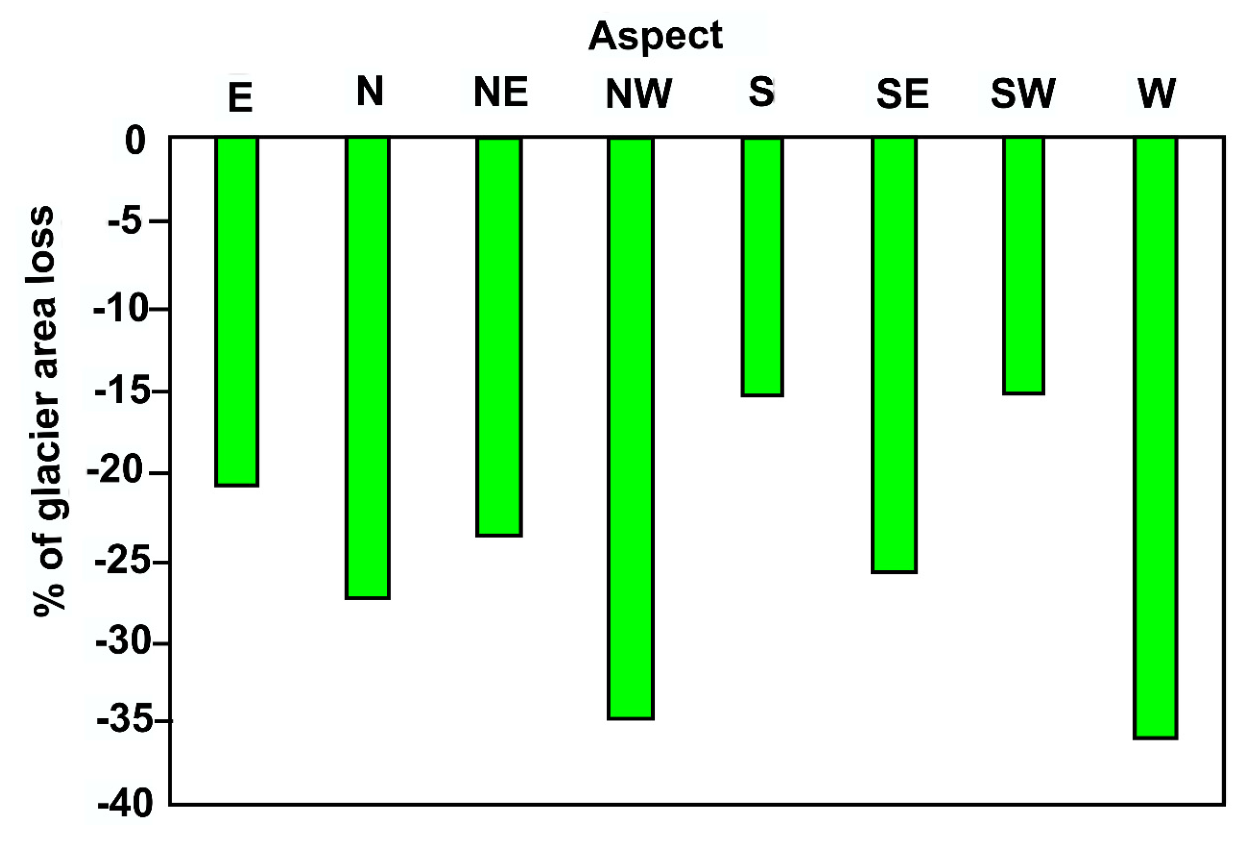
This study records that the maximum percentage of glaciers receded from the western (36%) and north-western aspects (35%), but relatively lesser in the southern (15%) and south-western (15%) aspects (Figure 15). Therefore, specific aspects reveals themselves as vital determinants of deglaciation in the CKB, probably supporting the assumption that the glaciers are of the Summer Accumulation Type.
Altitude governs the rates of melting of glacier ice [50]. A negative correlation (significant at the 0.0001 level) (Supplementary Table S7) has been found to existbetween the percentage of glacier area loss and the lowest altitude. This relationship indicates that the glaciers extending to a lower altitude are prone to lose more glacier mass than the ones perched on higher altitudes, barring the niche type smaller ice bodies. It may be related to the capacity of the lower denser altitudinal atmosphere to hold more heat energy than the upper lighter ones [61].
6. Conclusions
This research presents a semi-automated clean glacier and debris-covered glacier delineation and data, for the Changme Khangpu Basin. The two maps, i.e., 1. NIR/SWIR, and 2. Composite of LST, slope, and NDSI maps helped in delineating near accurate debris-covered boundary. This research provides an updated and comprehensive glacier inventory in the CKB as well, recording a total of 81 glaciers, covering an area of 75.78 ±1.54 km2. Glaciers are much smaller in this basin, with the size ranging from 0.03 to 13.79 km2. The input-output mechanism, along with seasonal control on these elements may be the reason for sustaining a higher number of smaller glaciers in this region as compared to the Western Himalayas. Frequency of glaciers and area distribution are markedly controlled by aspect, snout elevation, and average slope. About 73% of large-sized glaciers are concentrated on the southern, south-eastern and south-western aspect, with an average slope of ≤20°. Glaciers with supraglacial debris cover in the CKB are larger in size, and gentler in slope. Glaciers situated on the southern aspect have a strong connection with the SW monsoon, and as a result, average minimum altitude extends to the lower elevation (less than 5000 m) as compared to the other aspects.
About 20% of glacier area has been lost from the CKB at the rate of -0.507 ± 0.001% between 1975 and 2016. The regional level decadal late summer temperature and monsoon precipitation anomaly appear to be a determinants in glacial dynamics in this basin. The lower rate of glacier area shrinkage during 1988–2001 was followed by the highest rate of area loss in the recent decade (2001–2016). The lower (−0.170 ± 0.536 km2a−1) retreat during 1988–2001 might have been as a result of regional level late-summer temperature fall, and a peak in monsoon precipitation in the early 1990s. The early 21st century late-summer warming probably triggered the recession at a faster pace (−0.665 ± 0.243 km2a−1), but cannot be the only concluding reason. Besides, glacial dynamics in the CKB are controlled by the local topographic parameters. The western and north-western aspects show more recession as compared to the other aspects. The study reveals that clean glaciers have nearly twice the rate of recession as compared to debris-covered glaciers. One of the debris-covered benchmark glaciers, Changme Khangpu (CK) receded at the rate of −4.4 ma−1. The future research on debris-covered area and supraglacial pond dynamics can provide precise information on the climate–glacier interplay in the similar regions.
Supplementary Materials
The following are available online at https://www.mdpi.com/2076-3263/9/6/259/s1, Table S1: List of five 5th order basin of Tista, Table S2: Details of Inventoried glaciers in the CKB, India (2016), Table S3: Correlation between glacier size (km2) and minimum elevation (m) of glaciers, Table S4: Correlation between glacier size (km2) and mean slope of glaciers, Table S5: Significance test statistics for glacier area change (1975–2016), Table S6: Correlation between glacier size (km2) and glacier area change (1975–2016), Table S7: Correlation between glaciers minimum elevation (m) and percentage of glacier area change (1975–2016).
Author Contributions
All of the authors have given significant contributions to prepare this research paper. Being the subject mentor and joint-supervisor, the conceptualization of this research was flourished by M.C.S. M.C.S, also, has given significant contribution in the investigation, project administration, supervision, validation, visualization, and performed the rigorous effort in the writing-review and editing. M.D., a pupil of M.C.S. and H.J.S., has gathered resources, software, data curation, and also has done the formal analysis, methodology development, and the writing-original draft. H.J.S., being an academic supervisor and mentor, contributed in the project administration, supervision, validation, visualization, and also gave enormous effort in the writing-review & editing. Both of the supervisors assisted in the funding acquisition to publish this research paper in the reputed open access journal.
Funding
We acknowledge the Council of Scientific and Industrial Research - University Grants Commission (CSIR-UGC), India, for providing a Senior Research Fellowship (SRF) to conduct this research (Sr. no. 206142040).
Acknowledgments
Authors would like to thank the USGS for free access to Landsat archive and SRTM data. Authors are grateful to the Govt. of Sikkim, India, for granting permission to conduct field survey in the study area, and Uttam Lal of the Department of Geography, at Sikkim University, for initiating and providing logistics for the field survey, under the IUCCC project of the DST, Govt. of India. We are also thankful to Parvendra Kumar of the Department of General & Applied Geography, HS Gour Central University Sagar, India, and Arindam Chowdhury of the Department of Geography, North-Eastern Hill University, India, for assisting in the field survey. Besides, we are expressing our sincere gratitude to the respected reviewers and the assistant editor of the journal, for their ample suggestions to enhance the paper writing.
Conflicts of Interest
The authors declare no conflict of interest.
References
- Haeberli, W.; Hoelzle, M.; Paul, F.; Zemp, M. Integrated monitoring of mountain glaciers as key indicators of global climate change: the European Alps. Ann. Glaciol. 2007, 46, 150–160. [Google Scholar] [CrossRef] [Green Version]
- Veettil, B.K.; Wang, S. An update on recent glacier changes in Mexico using Sentinel-2A data. Geogr. Ann. Ser. A Phys. Geogr. 2018, 100, 307–318. [Google Scholar] [CrossRef]
- Williams, M.W. The Status of Glaciers in the Hindu Kush – Himalayan Region. Mt. Res. Dev. 2013, 33, 114–115. [Google Scholar] [CrossRef]
- Haireti, A.; Tateishi, R.; Alsaaideh, B.; Gharechelou, S. Multi -criteri a techn nique for mapping of debris- covered and clean- ice glaciers in Shaksgam valley using Landsat TM and ASTER GDEM. J. Mt. Sci 2016, 13, 703–714. [Google Scholar] [CrossRef]
- Bahuguna, I.M.; Rathore, B.P.; Brahmbhatt, R.; Sharma, M.; Dhar, S.; Randhawa, S.S.; Kumar, K.; Romshoo, S.; Shah, R.D.; Ganjoo, R.K.; et al. Are the Himalayan glaciers retreating? Curr. Sci. 2014, 106, 1008–1013. [Google Scholar]
- Qureshi, M.A.; Yi, C.; Xu, X.; Li, Y. Glacier status during the period 1973 e 2014 in the Hunza Basin, Western Karakoram. Quat. Int. 2017, 444, 125–136. [Google Scholar] [CrossRef]
- Raj, K.B.G.; Rao, V.V.N.; Kumar, K.V.; Diwakar, P.G. Alarming recession of glaciers in Bhilangna basin, Garhwal Himalaya, from 1965 to 2014 analysed from Corona and Cartosat data. Geomat. Nat. Hazards Risk 2017, 8, 1424–1439. [Google Scholar] [Green Version]
- Chand, P.; Sharma, M.C. Glacier changes in the Ravi basin, North-Western Himalaya (India) during the last four decades (1971-2010/13). Glob. Planet. Chang. 2015, 135, 133–147. [Google Scholar] [CrossRef]
- Bajracharya, S.R.; Shrestha, B. The Status of Glaciers in the Hindu Kush-Himalayan Region; International Centre for Integrated Mountain Development (ICIMOD): Kathmandu, Nepal, 2011; ISBN 978 92 9115 217. [Google Scholar]
- Dobreva, I.D.; Bishop, M.P.; Bush, A.B.G. Climate-glacier dynamics and topographic forcing in the Karakoram Himalaya: Concepts, issues and research directions. Water 2017, 9, 405. [Google Scholar] [CrossRef]
- Thompson, S.; Benn, D.I.; Mertes, J.; Luckman, A. Stagnation and mass loss on a Himalayan debris-covered glacier: Processes, patterns and rates. J. Glaciol. 2016, 62, 467–485. [Google Scholar] [CrossRef]
- Robson, B.A.; Nuth, C.; Nielsen, P.R.; Girod, L.; Hendrickx, M. Spatial Variability in Patterns of Glacier Change across the Manaslu Range, Central Himalaya. Front. Earth Sci. 2018, 6, 1–19. [Google Scholar] [CrossRef]
- Das, S.; Sharma, M.C. Glacier changes between 1971 and 2016 in the Jankar Chhu Watershed, Lahaul Himalaya, India. J. Glaciol. 2018, 1–16. [Google Scholar] [CrossRef]
- Raina, V.K.; Srivastava, D. Glacier Atlas of India; Geological Survey of India: Bangalore, India, 2008.
- Fujita, K.; Ageta, Y. Effect of summer accumulation on glacier mass balance on the Tibetan Plateau revealed by mass-balance model. J. Glaciol. 2000, 46, 244–252. [Google Scholar] [CrossRef] [Green Version]
- Salerno, F.; Thakuri, S.; Tartari, G.; Nuimura, T.; Sunako, S.; Sakai, A.; Fujita, K. Debris-covered glacier anomaly? Morphological factors controlling changes in the mass balance, surface area, terminus position, and snow line altitude of Himalayan glaciers. Earth Planet. Sci. Lett. 2017, 471, 19–31. [Google Scholar] [CrossRef]
- Thakuri, S.; Salerno, F.; Smiraglia, C.; Bolch, T.; D’Agata, C.; Viviano, G.; Tartari, G. Tracing glacier changes since the 1960s on the south slope of Mt. Everest (central Southern Himalaya) using optical satellite imagery. Cryosphere 2014, 8, 1297–1315. [Google Scholar] [CrossRef] [Green Version]
- Debnath, M.; Syiemlieh, H.J.; Sharma, M.C.; Kumar, R.; Chowdhury, A.; Lal, U. Glacial lake dynamics and lake surface temperature assessment along the Kangchengayo-Pauhunri Massif, Sikkim Himalaya, 1988–2014. Remote Sens. Appl. Soc. Environ. 2018, 9, 26–41. [Google Scholar] [CrossRef]
- Mann, H.B. Nonparametric Tests Against Trend. Econometrica 1945, 13, 245–259. [Google Scholar] [CrossRef]
- Kendall, M.G. Rank Correlation Methods, 4th ed.; Charles Griffin: London, UK, 1975. [Google Scholar]
- Bookhagen, B.; Burbank, D.W. Topography, Relief, and TRMM-derived rainfall variations along the Himalaya. Geophys. Res. Lett. 2006, 33, 17–18. [Google Scholar]
- Chaturvedi, R.K.; Kulkarni, A.V.; Karyakarte, Y.; Govindasamy, B. Glacial mass balance changes in the Karakoram and Himalaya based on CMIP5 multi-model climate projections Glacial mass balance changes in the Karakoram and Himalaya based on CMIP5 multi-model. Clim. Chang. 2014, 123. [Google Scholar] [CrossRef]
- Sakai, A.; Nuimura, T.; Fujita, K.; Takenaka, S.; Nagai, H.; Lamsal, D. Climate regime of Asian glaciers revealed by GAMDAM glacier inventory. Cryosphere 2015, 9, 865–880. [Google Scholar] [CrossRef] [Green Version]
- NASA Landsat 7 science data user’s handbook. Available online: https://landsat.gsfc.nasa.gov/landsat-7-science-data-users-handbook/ (accessed on 25 May 2019).
- USGS Landsat 8 (L8) Data Users Handbook Version 1.0 June 2015. Available online: https://www.usgs.gov/land-resources/nli/landsat/landsat-8-data-users-handbook (accessed on 25 May 2019).
- Usmanova, Z.; Shahgedanova, M.; Severskiy, I.; Nosenko, G.; Kapitsa, V. Assessment of Glacier Area Change in the Tekes River Basin, Central Tien Shan, Kazakhstan Between 1976 and 2013 Using Landsat and KH-9 Imagery. Cryosph. Discuss. 2016, 1–47. [Google Scholar] [CrossRef]
- Padmanabha, E.A.; Shashivardhan, P.; Shashivardhan, P.; Shashivardhan Reddy, P.; Narender, B.; Muralikrishnan, S.; Dadhwal, V.K. Photogrammetric processing of hexagon stereo data for change detection studies. ISPRS Ann. Photogramm. Remote Sens. Spat. Inf. Sci. 2014, II-8, 151–157. [Google Scholar] [CrossRef] [Green Version]
- Surazakov, A.; Aizen, V. Positional accuracy evaluation of declassified Hexagon KH-9 mapping camera imagery. Photogramm. Eng. Remote Sens. 2010, 5, 603–608. [Google Scholar] [CrossRef]
- Bolch, T.; Kamp, U. Glacier Mapping in High Mountains Using DEMs, Landsat and ASTER Data, Proceedings of the 8th International Symposium on High Mountain Remote Sensing Cartography, La Paz, Bolivia, 20–27 March 2005; Kaufmann, V., Sulzer, W., Eds.; Karl Franzens University: Graz, Austria, 2006; pp. 13–24. [Google Scholar]
- Racoviteanu, A.E.; Arnaud, Y.; Williams, M.W.; Ordoñez, J. Decadal changes in glacier parameters in the Cordillera Blanca, Peru, derived from remote sensing. J. Glaciol. 2008, 54, 499–510. [Google Scholar] [CrossRef] [Green Version]
- Racoviteanu, A.E.; Paul, F.; Raup, B.; Khalsa, S.J.S.; Armstrong, R. Challenges and recommendations in mapping of glacier parameters from space: Results of the 2008 global land ice measurements from space (GLIMS) workshop, Boulder, Colorado, USA. Ann. Glaciol. 2010, 50, 53–69. [Google Scholar] [CrossRef]
- Paul, F.; Huggel, C.; Kääb, A. Combining satellite multispectral image data and a digital elevation model for mapping debris-covered glaciers. Remote Sens. Environ. 2004, 89, 510–518. [Google Scholar] [CrossRef]
- Bhambri, R.; Bolch, T.; Chaujar, R.K.; Kulshreshtha, S.C. Glacier changes in the Garhwal Himalaya, India, from 1968 to 2006 based on remote sensing. J. Glaciol. 2011, 57, 543–556. [Google Scholar] [CrossRef] [Green Version]
- Pratibha, S.; Kulkarni, A.V. Decadal change in supraglacial debris cover in Baspa basin, Western Himalaya. Curr. Sci. 2018, 114, 25–30. [Google Scholar] [CrossRef]
- Ka, A.; Bolch, T.; Casey, K.; Heid, T.; Kargel, J.S.; Leonard, G.J.; Paul, F.; Raup, B.H. Glacier mapping and monitoring using multispectral data. Glob. Land Ice Meas. Space 2014, 75–112. [Google Scholar] [CrossRef]
- Casey, K.A.; Kääb, A.; Benn, D.I. Characterization of glacier debris cover via in situ and optical remote sensing methods: a case study in the Khumbu. Cryosph. Discuss. 2011, 5, 499–564. [Google Scholar] [CrossRef]
- Bolch, T.; Buchroithner, M.; Kunert, A.; Kamp, U. Automated Delineation of Debris-Covered Glaciers Based on ASTER Data. In Proceedings of the 27th EARSel Symp, Bozen, Italy, 4–7 June 2007; pp. 403–410. [Google Scholar]
- Alifu, H.; Tateishi, R.; Johnson, B. A new band ratio technique for mapping debris-covered glaciers using Landsat imagery and a digital elevation model. Int. J. Remote Sens. 2015, 36, 2063–2075. [Google Scholar] [CrossRef]
- Gillespie, A. Land Surface Emissivity. In Encyclopedia of Remote Sensing; Njoku, E.G., Ed.; Springer: New York, NY, USA, 2016; pp. 401–402. [Google Scholar]
- Sobrino, J.A.; Jiménez-Muñoz, J.C.; Sòria, G.; Romaguera, M.; Guanter, L.; Moreno, J.; Plaza, A.; Martínez, P. Land surface emissivity retrieval from different VNIR and TIR sensors. IEEE Trans. Geosci. Remote Sens. 2008, 46, 316–327. [Google Scholar] [CrossRef]
- Wang, F.; Qin, Z.; Song, C.; Tu, L.; Karnieli, A.; Zhao, S. An improved mono-window algorithm for land surface temperature retrieval from landsat 8 thermal infrared sensor data. Remote Sens. 2015, 7, 4268–4289. [Google Scholar] [CrossRef]
- Whalley, W.B.; Azizi, F. Rock glaciers and protalus landforms: Analogous forms and ice sources on Earth and Mars. J. Geophys. Res. 2003, 108, 1–17. [Google Scholar] [CrossRef]
- Granshaw, F.D.; Fountain, A.G. Glacier change (1958–1998) in the North Cascades National Park Complex, Washington, USA Frank. J. Glaciol. 2006, 52, 251–256. [Google Scholar] [CrossRef]
- Bolch, T.; Menounos, B.; Wheate, R. Landsat-based inventory of glaciers in western Canada, 1985-2005. Remote Sens. Environ. 2010, 114, 127–137. [Google Scholar] [CrossRef]
- Bolch, T.; Yao, T.; Kang, S.; Buchroithner, M.F.; Scherer, D.; Maussion, F.; Huintjes, E.; Schneider, C. A glacier inventory for the western Nyainqentanglha range and the Nam Co Basin, Tibet, and glacier changes 1976–2009. Cryosphere 2010, 4, 419–433. [Google Scholar] [CrossRef]
- Hall, D.K.; Bayr, K.J.; Schöner, W.; Bindschadler, R.A.; Chien, J.Y.L. Consideration of the errors inherent in mapping historical glacier positions in Austria from the ground and space (1893-2001). Remote Sens. Environ. 2003, 86, 566–577. [Google Scholar] [CrossRef]
- Wang, X.; Chen, H.; Chen, Y. Topography-Related Glacier Area Changes in Central Tianshan from 1989 to 2015 Derived from Landsat Images and ASTER GDEM Data. Water 2018, 10. [Google Scholar] [CrossRef]
- Li, Y.; Li, Y. Topographic and geometric controls on glacier changes in the central Tien Shan, China, since the Little Ice Age. Ann. Glaciol. 2014, 55, 177–186. [Google Scholar] [CrossRef] [Green Version]
- Nagai, H.; Fujita, K.; Nuimura, T.; Sakai, A. Southwest-facing slopes control the formation of debris-covered glaciers in the Bhutan Himalaya. Cryosphere 2013, 7, 1303–1314. [Google Scholar] [CrossRef] [Green Version]
- Brahmbhatt, R.M.; Bahuguna, I.M.; Rathore, B.P.; Kulkarni, A.V.; Shah, R.D.; Rajawat, A.S.; Kargel, J.S. Significance of glacio-morphological factors in glacier retreat: a case study of part of Chenab basin, Himalaya. J. Mt. Sci. 2017, 14, 128–141. [Google Scholar] [CrossRef]
- Bhattacharyya, A.; Chaudhary, V. Late-Summer Temperature Reconstruction of the Eastern Himalayan Region Based on Tree-Ring Data of Abies densa. Arctic, Antarct. Alp. Res. 2006, 35, 196–202. [Google Scholar] [CrossRef]
- Yadava, A.K.; Yadav, R.R.; Misra, K.G.; Singh, J. Tree ring evidence of late summer warming in Sikkim, northeast India. Quat. Int. 2015, 371, 175–180. [Google Scholar] [CrossRef]
- Borgaonkar, H.P.; Gandhi, N.; Ram, S.; Krishnan, R. Tree-ring reconstruction of late summer temperatures in northern Sikkim (eastern Himalayas). Palaeogeogr. Palaeoclimatol. Palaeoecol. 2018, 504, 125–135. [Google Scholar] [CrossRef]
- Ojha, S.; Fujita, K.; Sakai, A.; Nagai, H.; Lamsal, D. Topographic controls on the debris-cover extent of glaciers in the Eastern Himalayas: Regional analysis using a novel high-resolution glacier inventory. Quat. Int. 2017, 455, 82–92. [Google Scholar] [CrossRef]
- Bolch, T.; Kulkarni, A.; Kääb, A.; Huggel, C.; Paul, F.; Cogley, J.G.; Fujita, K.; Scheel, M.; Bajracharya, S.; Stoffel, M. The State and Fate of Himalayan Glaciers. Science 2012, 336, 310–314. [Google Scholar] [CrossRef] [Green Version]
- Kulkarni, A.V.; Rathore, B.P.; Singh, S.K.; Bahuguna, I.M. Understanding changes in the Himalayan cryosphere using remote sensing techniques. Int. J. Remote Sens. 2011, 32, 601–615. [Google Scholar] [CrossRef]
- Benn, D.I.; Kirkbride, M.P.; Owen, L.A.; Brazier, V. Glaciated Valley Landsystems. In Glacial Landsystems; Evans, D.J.A., Ed.; Hodder Arnold: London, UK, 2005; pp. 372–406. [Google Scholar]
- Benn, D.; Bolch, T.; Hands, K.; Kingdom, U.; Gulley, J.; Luckman, A.; Nicholson, L.I.; Quincey, Q.; Thompson, S.; Toumi, R.; et al. Response of debris-covered glaciers in the Mount Everest region to recent warming, and implications for outburst flood hazards. Earth-Sci. Rev. 2012, 114, 156–174. [Google Scholar] [CrossRef] [Green Version]
- Watson, C.S.; Quincey, D.J.; Carrivick, J.L.; Smith, M.W.; Richardson, R. Heterogeneous water storage and thermal regime of supraglacial ponds on debris-covered glaciers. Earth Surf. Process. Landforms 2018, 43, 229–241. [Google Scholar] [CrossRef]
- Sakai, A.; Takeuchi, N.; Fujita, K.; Nakawo, M. Role of supraglacial ponds in the ablation process of a debris-covered glacier in the Nepal Himalayas. IAHS Publ. 2000, 265, 119–130. [Google Scholar]
- Benn, D.I.; Evans, D.J.A. Glaciers & Glaciation, 2nd ed.; Hodder Education: London, UK, 2010. [Google Scholar]
Figure 1.
Location map of the study region: Changme Khangpu basin is located in the north-eastern part of Sikkim, a part of Eastern Himalaya, India.
Figure 1.
Location map of the study region: Changme Khangpu basin is located in the north-eastern part of Sikkim, a part of Eastern Himalaya, India.

Figure 2.
Climograph of North District, Sikkim represents average monthly data from 1901 to 2002; Data Source: India Water Portal (https://www.indiawaterportal.org/met_data/).
Figure 2.
Climograph of North District, Sikkim represents average monthly data from 1901 to 2002; Data Source: India Water Portal (https://www.indiawaterportal.org/met_data/).

Figure 3.
Parameters used for glacier boundary delineation: (a) NDSI map, (b) slope map (in °), (c) aspect map, (d) land surface temperature map (in °C), (e) NIR/SWIR map, (f) Composite map of LST, the glacier boundary modified from the International Centre for Integrated Mountain Development (ICIMOD) (2011) draped on (a–e) map, the (f) map contains the ICIMOD (2011) and 2016 glacier boundary. The dashed rectangular boxes in (e) and (f) map highlights the debris covered boundary of CK glacier.

Figure 4.
Distribution of glaciers (2016) (a) box-whisker plot of glacier surface area. The words SW, SE and S represent aspect of south-west, south-east and south, respectively; (b) histogram of glacier distribution; (c) normal Q-Q plot of glaciers.
Figure 4.
Distribution of glaciers (2016) (a) box-whisker plot of glacier surface area. The words SW, SE and S represent aspect of south-west, south-east and south, respectively; (b) histogram of glacier distribution; (c) normal Q-Q plot of glaciers.
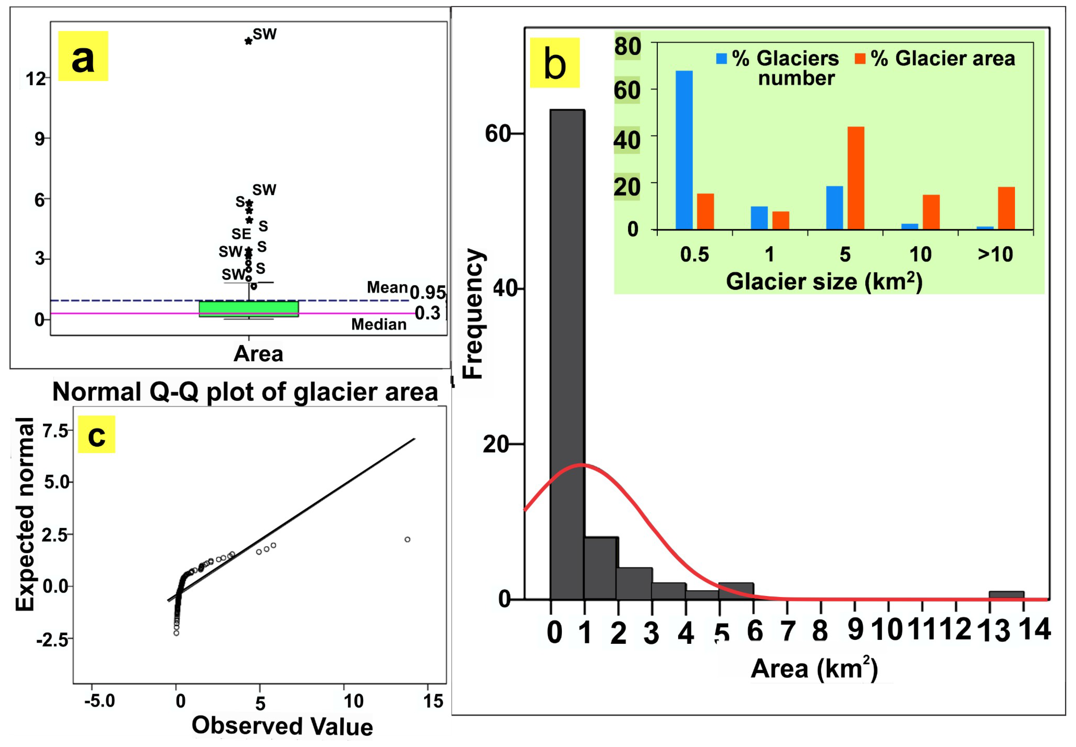
Figure 5.
Differences between glacier outlines delineated by ICIMOD (2011) and the present study of the periods 2001 (LANDSAT ETM+) and 2016 (LANDSAT OLI-TIRS): (a) The 2001 glacier boundary and ICIMOD glacier boundary (2011) have been draped on the LANDSAT ETM+ (2001) image, (b) 2016 glacier boundary and ICIMOD (2011) have been draped on the LANDSAT OLI-TIRS image (2014).
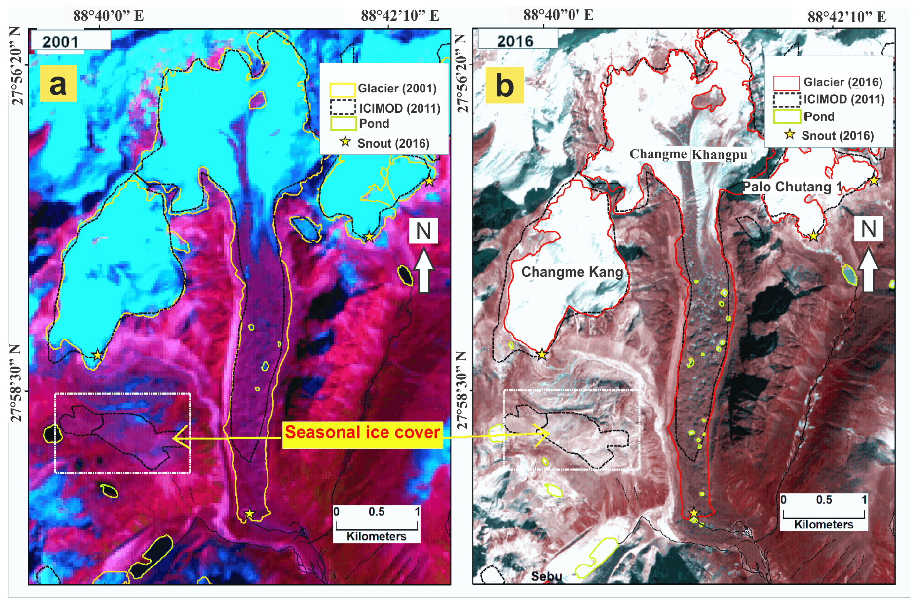
Figure 6.
Aspect-wise distribution of glacier area and frequency (2016). (a) Glacier area distribution on different aspects with median line (red color) and extreme values, (b) Percentage of glacier frequency and glacier area according to aspect.
Figure 6.
Aspect-wise distribution of glacier area and frequency (2016). (a) Glacier area distribution on different aspects with median line (red color) and extreme values, (b) Percentage of glacier frequency and glacier area according to aspect.

Figure 7.
The niche glaciers developed on the northern slope, (a) field photograph (November 2015) of two niche glaciers developed on a single mountain slope separated by an Arête (red dashed line); (b) field photograph (November 2018) of the side face of niche-1 glacier; (c) field photograph (November 2016) of a fresh talus cone spread below the snout of the niche-1 glacier and the toe being truncated by the stream (Sebu Chu) (blue dashed line).

Figure 8.
Box-whisker graphs plotted on the different aspects; (a) glaciers minimum elevations and (b) average slope of glaciers. Star mark in both graphs signify extreme values.
Figure 8.
Box-whisker graphs plotted on the different aspects; (a) glaciers minimum elevations and (b) average slope of glaciers. Star mark in both graphs signify extreme values.

Figure 9.
Division of glaciers according to debris cover in the ablation zone; (a) frequency distribution (in percentage) of glaciers according to type (excluding the rock glaciers), (b) proportion of area according to the glacier type.
Figure 9.
Division of glaciers according to debris cover in the ablation zone; (a) frequency distribution (in percentage) of glaciers according to type (excluding the rock glaciers), (b) proportion of area according to the glacier type.

Figure 10.
Field photograph of the upper reaches of the debris-covered glacier CK lateral moraines (red polygons) enclosing the glacier; the black dashed separation line marking the accumulation area (AC), in the upper part and debris-covered ablation area (AB), in the lower part; the avalanche cones (magenta colored polygons).

Figure 11.
Rock glaciers (RG) in the CKB; (a) The RG-1 on the gentle slope. The RG-2 transformed from the initial laterofrontal moraine; (b) field photograph (November, 2016) showing the fresh scree on the mountain slope which is descending from the RG-1; (c) thermokarst pond (P).
Figure 11.
Rock glaciers (RG) in the CKB; (a) The RG-1 on the gentle slope. The RG-2 transformed from the initial laterofrontal moraine; (b) field photograph (November, 2016) showing the fresh scree on the mountain slope which is descending from the RG-1; (c) thermokarst pond (P).
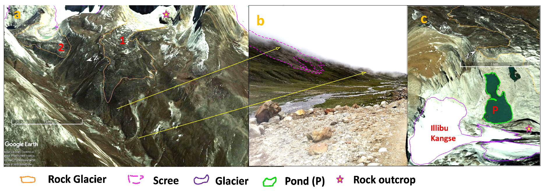
Figure 12.
The bar graphs represent glacier area dynamics: 1975–2016, 1975–1988, 1988–2001, 2001–2016 (a) percentage of total glacier area changes (b) Rate of total glacier area recession (c) Percentage of glacier area recession, and rate of glacier area recession according to the type of glaciers.
Figure 12.
The bar graphs represent glacier area dynamics: 1975–2016, 1975–1988, 1988–2001, 2001–2016 (a) percentage of total glacier area changes (b) Rate of total glacier area recession (c) Percentage of glacier area recession, and rate of glacier area recession according to the type of glaciers.

Figure 13.
Fragmentation of a glacier into two. Different set of underlying images are: (a) Corona image (1975); (b) LANDSAT TM (1988); (c) LANDSAT ETM+ (2001); (d) Sentinel 2A (2016).
Figure 13.
Fragmentation of a glacier into two. Different set of underlying images are: (a) Corona image (1975); (b) LANDSAT TM (1988); (c) LANDSAT ETM+ (2001); (d) Sentinel 2A (2016).

Figure 14.
(a) Snout position and snout area changes of the CK glacier since 1975 to 2016. Base map: Sentinel 2A; (b) supraglacial ponds on the debris-covered ablation zone of CK glacier; (c) southernmost (No. 1) supraglacial pond (1410 m2 area) covered by debris.
Figure 14.
(a) Snout position and snout area changes of the CK glacier since 1975 to 2016. Base map: Sentinel 2A; (b) supraglacial ponds on the debris-covered ablation zone of CK glacier; (c) southernmost (No. 1) supraglacial pond (1410 m2 area) covered by debris.

Figure 15.
Varying percentage of glacier area loss on different aspects.

Table 1.
Long-term (1950–2016) trend analysis of monthly precipitation and temperature in the Changme Khangpu Basin; Data Source: (http://www.cru.uea.ac.uk/data).
Table 1.
Long-term (1950–2016) trend analysis of monthly precipitation and temperature in the Changme Khangpu Basin; Data Source: (http://www.cru.uea.ac.uk/data).
| Precipitation | Temperature | |||||
|---|---|---|---|---|---|---|
| Season | Kendall’s Tau | Level of Significance | Sen’s Slope (mm a−1) | Kendall’s Tau | Level of Significance | Sen’s Slope (°C a−1) |
| Winter | 0.165 | 0.027 | 0.188 | 0.264 | 0.001 | 0.014 |
| Pre-monsoon | 0.266 | 0.001 | 1.083 | 0.232 | 0.003 | 0.019 |
| Monsoon | 0.001 | 0.498 | 0.010 | 0.381 | <0.0001 | 0.021 |
| Post-monsoon | 0.019 | 0.415 | 0.061 | 0.339 | <0.0001 | 0.027 |
Table 2.
Details of the data set.
| Satellite Sensors | Acquired Date | Repeat Coverage Interval (Days) | Spatial Resolution |
|---|---|---|---|
| Declassified Hexagon (KH9) | 20 February 1975 | N.A. | 8 m |
| LANDSAT TM | 1 December 1988 | 16 | MS* & TIRS* (30 m) |
| LANDSAT ETM+ | 26 October 2001 | 16 | MS* & TIRS*(30 m); Pan* (15 m) |
| LANDSAT OLI-TIRS | 7 Novermber 2014 | 16 | MS* (30 m); TIRS*(100 m); Pan* (15 m) |
| Sentinel-2A | 6 January 2016 | 5 | 10 m |
| Google Earth Images | 2015–2016 | N.A. | 1.65 to 2.62 m |
| SRTM DEM | 11–22 February 2000 | N.A. | 30 m |
| CRU temperature & Precipitation | 1950–2014 | N.A. | 0.50° × 0.50° |
| Monthly Temperature and Precipitation (India Waterportal) | 1901–2002 | N.A. | In situ |
| Swiss Foundation For Alpine Research’s map of Sikkim Himalaya | 1981 | N.A. | 1:150,000 |
Note: SRTM DEM refers to Shuttle Radar Topography Mission digital elevation model; CRU refers to Climate Research Unit; TM refers to Thematic Mapper; ETM+ refers to Enhanced Thematic Mapper Plus; MS denotes multispectral bands; TIRS denotes Thermal Infrared Sensor bands; Pan denotes Panchromatic band.
Table 3.
Tests of Normality of glacier distribution.
| General Statistics of Glacier Area in 2016 | |||
|---|---|---|---|
| N | 81 | ||
| Skewness | 4.741 | ||
| Std. Error of Skewness | 0.269 | ||
| Kurtosis | 28.453 | ||
| Std. Error of Kurtosis | 0.532 | ||
| Shapiro-Wilk | |||
| Statistic | df | Sig. | |
| Area | 0.476 | 81 | 0.000 |
Note: N, frequency of glaciers.
Table 4.
Nature of glacier area change during the study period (1975–2016).
| Period | % of Area Change | Rate of Change (km2·a−1) | Uncertainty of Rate of Area Change |
|---|---|---|---|
| 1975–2016 | −20.72 (±3.25) | −0.453 | ±0.001 |
| 2001–2016 | −11.84 (±4.51) | −0.665 | ±0.243 |
| 1988–2001 | −3.97 (±8.01) | −0.170 | ±0.536 |
| 1975–1988 | −6.35 (±7.37) | −0.491 | ±0.499 |
Note: *AC denotes the term of area change of glaciers.
Table 5.
Variation in glacier area shrinkage according to glacier types based on debris cover.
| Tot. Glacier Area (1975) | Tot. Glacier Area Change 1975–2016 | % of AC 1975–2016 | Rate of % of AC 1975–2016 | Rate AC 1975–2016 | Rate AC 1975–1988 | Rate AC 1988–2001 | Rate AC 2001–2016 | |
|---|---|---|---|---|---|---|---|---|
| Debris free | 51.451 | −13.032 | −25.329 | −0.618 | −0.318 | −0.244 | −0.149 | −0.528 |
| Maximum Debris covered | 23.887 | −3.685 | −15.426 | −0.376 | −0.090 | −0.136 | −0.016 | −0.114 |
| Partly debris covered | 17.419 | −2.578 | −14.801 | −0.361 | −0.063 | −0.111 | −0.016 | −0.062 |
*TA, TAC, AC denotes the term of total area, total area change and area change of glaciers, respectively.
© 2019 by the authors. Licensee MDPI, Basel, Switzerland. This article is an open access article distributed under the terms and conditions of the Creative Commons Attribution (CC BY) license (http://creativecommons.org/licenses/by/4.0/).
Share and Cite
MDPI and ACS Style
Debnath, M.; Sharma, M.C.; Syiemlieh, H.J. Glacier Dynamics in Changme Khangpu Basin, Sikkim Himalaya, India, between 1975 and 2016. Geosciences 2019, 9, 259. https://doi.org/10.3390/geosciences9060259
AMA Style
Debnath M, Sharma MC, Syiemlieh HJ. Glacier Dynamics in Changme Khangpu Basin, Sikkim Himalaya, India, between 1975 and 2016. Geosciences. 2019; 9(6):259. https://doi.org/10.3390/geosciences9060259
Chicago/Turabian StyleDebnath, Manasi, Milap Chand Sharma, and Hiambok Jones Syiemlieh. 2019. "Glacier Dynamics in Changme Khangpu Basin, Sikkim Himalaya, India, between 1975 and 2016" Geosciences 9, no. 6: 259. https://doi.org/10.3390/geosciences9060259
Note that from the first issue of 2016, this journal uses article numbers instead of page numbers. See further details here.