Generation of Sub-Hourly Rainfall Events through a Point Stochastic Rainfall Model

Abstract

The aim of this paper is to present a stochastic model to generate sub-hourly rainfall events at a given point. Historical events used as the input have been extracted by the sub-hourly rainfall series available for a defined rain gauge station based on a fixed inter-event time and selected if their average intensity was larger than a critical fixed one. The sub-hourly events generated by applying the proposed methodology are completely stochastic and their main characteristics, i.e., shape, duration and average intensity, have been derived as a function of the statistics of the historical events analyzed. In order to characterize the shape, dimensionless hyetographs have been derived. They have been statistically modelled by using the Beta cumulative distribution. Average intensity and duration of the historical events were first modelled separately by fitting several probability distributions and selecting the best one using the more common statistical criteria. Then, their correlation was modelled using the Frank’s copula. In order to test the methodology, two sites in Sicily, Italy, where 10 min’ recorded rainfall data were available, were analyzed. Finally, comparison between the statistics of the simulated events and those of the measured data demonstrates the good performance of the model.

1. Introduction

The simulation of sub-hourly rainfall events is an important field of hydrological research [1,2], being mainly useful for, e.g., designing water control structures in urban areas or urban drainage systems, and for flood frequency evaluations in small natural catchments, characterized by rapid hydrological response [3,4].

For these purposes, the availability of a long sample of high temporal-resolution rainfall events (shorter than 1 h) is necessary. However, unfortunately, long series of recorded rainfall characterized by high temporal resolution are not available in most of the rain gauge stations in Sicily. Usually, if long series of rainfall data are available, their temporal resolution is often unfortunately lower than that required for the application of a statistical model; in contrast, if high-resolution rainfall data are available, their sample is often not sufficiently long to perform reliable statistical analyses. In these cases, the synthetic generation of long series of high-resolution rainfall events using stochastic point process representations of rainfall (e.g., through Monte Carlo approach) [5,6,7,8,9,10] can be a very practical alternative.

In the literature, there are two main groups of rainfall stochastic generation models: profile-based and pulse-based.

A profile-based model [7,11,12,13,14], i.e., those proposed by Eagleson [12], Blazkova and Beven [7] or Robinson and Sivapalan [14], is focused on a single rainfall event. These models generally characterize the rainfall event through the identification of the inter-event time and adopt joint or separate statistical distributions to describe the main characteristics of a storm event (duration and rainfall depth or, alternatively, duration and average intensity). The total volume of the considered rainfall event is then divided into discrete depth values at a specified time-step (e.g., 10 min) via i.e., mass curve [11,12,13].

The second type of model (pulse-based) characterizes storm occurrences as localized events distributed randomly in time and whose occurrences follow a Poisson process. Each rainfall event causes a cluster of rain cells, and every cell can be assumed as a pulse with a random duration and random intensity generally supposed to be constant throughout the cell duration. Cells are distributed in time according either to the Neyman–Scott cluster model [5,6,15,16] or Bartlett–Lewis cluster model [17,18,19,20]. Because of their ability to offer an accurate representation of continuous rainfall series, they can be very useful for several purposes in hydrology.

However, for their application, many parameters have to be estimated and a considerable size of historical rainfall data records has to be available in a continuous form. Moreover, as highlighted by Cameron et al. [2], although these models are able to reproduce with high accuracy the observed inter-arrival times characteristics at different timescales, their performance to simulate the extreme statistics at short timescales is less accurate. Consequently, several authors [1,7] suggested the possibility of using profile-based models for their case studies.

Following this latter type of models, we developed a methodology to derive stochastic sub-hourly rainfall events at a given point, easily applicable in several situations. The main advantage of the rainfall model here presented is that, for its implementation, it does not need of the availability of a considerable size of rainfall data. A few years of high-resolution rainfall data, non-necessarily continuous, are sufficient to calibrate the model.

Rainfall events, in terms of their main characteristics, i.e., duration and average intensity, are stochastically generated using a bivariate copula-based model, while in order to characterize the shape, dimensionless events (mass curves) have been considered. As highlighted by several authors [11,13,21,22], for a particular location or within a meteorologically homogeneous regions, temporal structure of storms is expected to exhibit similarities despite their different durations and total storm depth [22].

For those concerning duration and average intensity, Cordova and Rodriguez-Iturbe [23] demonstrated how for each location, a well-defined correlation structure exists between the main characteristics of an event, i.e., storm duration and rainfall intensity. Based on this study, many other authors have analyzed this correlation structure [24,25,26] by applying several bivariate distributions, thereby demonstrating that to assume these characteristics to be independent of each other is an unrealistic hypothesis [27].

In this context, the application of copula theory to analyze the statistical dependence between storm duration and rainfall intensity represents an effective choice [27,28,29]. The main advantage in the use of copulas is that the considered variables do not need to be independent of each other or to be modelled by the same kind of marginal distributions. In order to generate pairs of duration and average intensity, it is necessary to model these characteristics by using a statistical probability distribution, and then to link them by using a joint probability distribution, and in particular by using copulas [28,30,31,32,33].

A first version of the proposed methodology was already presented in a previous work by the authors [9]; that version, however, in the validation phase, showed some limitations, especially for the one concerning the historic events definition and separation, and for the rainfall’s temporal pattern characterization. Consequently, the model has been partially redesigned and it has been validated in order to overcome some of its shortcomings.

The model has been calibrated using the rainfall data collected in two different sites in Sicily, Italy. In both cases, recorded available rainfall series have been divided into wet and dry periods in function of a fixed inter-event time. Of all the historical rainfall events thus derived, only those that had average intensities larger than a fixed critical value were considered as input to the stochastic model of rainfall.

2. Stochastic Model of Rainfall

2.1. Overview

This section presents the layout of the proposed rainfall model structure. Following Vandenberghe et al. approach [34], the model consists of two main sections: after the statistical analysis of the main characteristics of the historical records, the first section performs the generation of pairs of duration and rainfall average intensity by using a bivariate copula model. The second one performs the generation of temporal patterns of rainfall through the statistical analysis of historical dimensionless hyetographs.

2.2. Rainfall Data

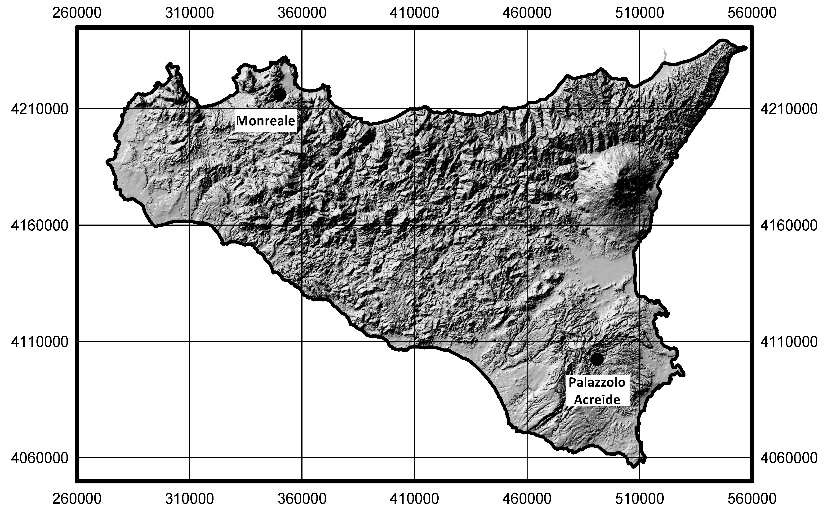
For the implementation of the model, 10 min rainfall data recorded in two sites located in Sicily have been considered (Figure 1). The rainfall data belong to the database of the “Servizio Informativo Agrometeorologico Siciliano” (SIAS; www.sias.regione.sicilia.it). The first site is Monreale rain gauge station, placed in the northwest part of the island, with data available in the period from 2003 to 2009. The second site is Palazzolo Acreide rain gauge station, placed in the southeast part of Sicily, with data available from the period from 2002 to 2007.

An average annual rainfall of 850 mm and 600 mm is observed for Monreale and Palazzolo Acreide rain gauge stations respectively. Climate pattern is the typical Mediterranean one with rainy season concentrated during the winter period and usually non-rainy days during the summer. As a consequence, all the rainfall events occur in 50–55 rainy days and, in terms of extreme events, an average value of about 13–15 significant rainfall events per year is observed [35].

2.3. Derivation of Rainfall Events

For the model implementation, it was first necessary to identify independent significant rainfall events in the collected time series. Rainfall registrations can be interpreted as rainfall sequences characterized by alternative wet periods, where a certain amount of rainfall is registered for each considered time step, and dry periods, where no rain or less than a certain amount of rain is registered for more consecutive time-steps. Wet periods are defined in function of their cumulative rainfall depth, duration and temporal pattern, while dry periods are characterized only by their duration. Wet and dry periods are separated from each other through the inter-event time definition.

The estimation of this time can differ greatly [7,22,27], depending in many cases on the model used for the rainfall analysis. The criteria used here, according to what proposed by Koutsoyiannis and Foufoula-Georgiou [21], is to define storms as rainfall events which are independent from each other, as based on Poisson storm arrivals. Here, the measure of the correlation between two successive events was evaluated by fitting an exponential distribution to the samples of rainfall depth-duration obtained separating the historical series for different inter-event time considered and checking the goodness of fit through the chi-square test application. The minimum inter-event time for which the chi-square test is satisfied is the inter-event time that has to be considered. Following this procedure, a minimum inter-event time that equals to 2 h for Monreale rain gauge station and to 4 h for Palazzolo Acreide rain gauge station has been recognized and adopted.

The second step of the analysis is the choice of those to be considered as hydrologically “significant” events for the possible formation of a flooding. Therefore, in order to carry out this analysis, it was decided, according to the Rahman et al. approach [36], to select only those rainfall episodes which average intensity was greater than a fixed threshold intensity. Following this approach, the threshold intensity can be calculated as function of the 2-year return time Intensity-Duration-Frequency (IDF) curve:

$$I_{D,thres}=\alpha ·I_{D,T=2}=\alpha ·a\left(T\right)·t^{\left(n-1\right)},$$

(1)

where α is the reduction factor and the I_{D,T = 2} is the IDF curve expressed with a classical two-parameters power law with parameters a (function of the return period) and n.

The 2-year return time IDF curve was estimated by applying the Two Components Extreme Value (TCEV) distribution [37], already adopted in Sicily for the statistical modelling of extreme rainfall [35]. In order to apply Equation (1), it was also necessary to determinate the reduction factor α. The use of an appropriate value of this parameter allowed us to select “significant” events, meaning that events with smaller intensity are not included. Here, the reduction factor α has been linked to the annual mean number of rainfall episodes quantified by the application of the TCEV, as outlined in [35].

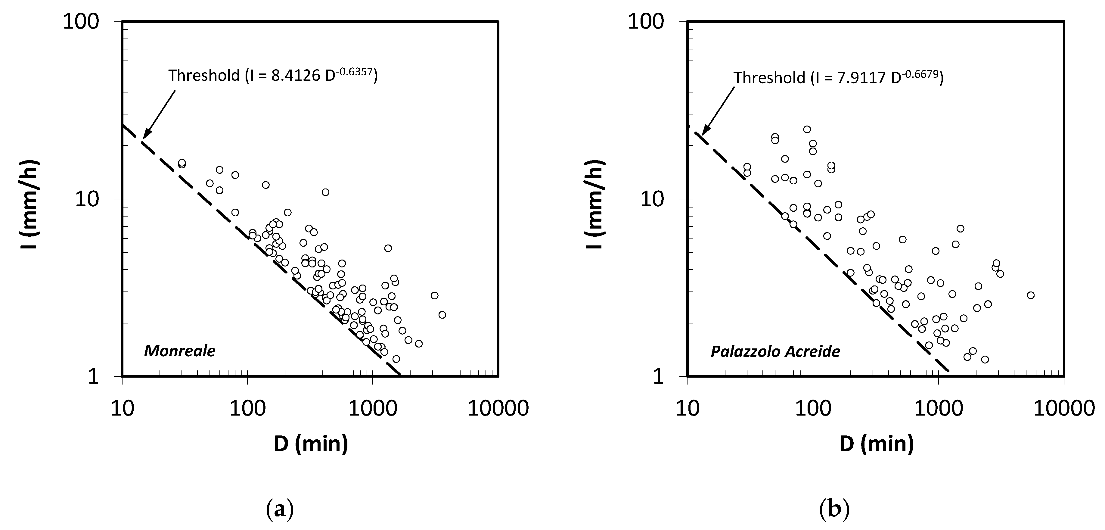
Following this, the annual mean number of rainfall episodes was estimated equals to about 15 for the Monreale rain gauge station and equals to about 13 for the Palazzolo Acreide rain gauge station. To ensure this average annual number of rainfall episodes, the value of the reduction factor α was set equal to 0.3 in both cases. With these assumptions, 105 independent rainfall events for Monreale and 83 independent rainfall events for Palazzolo Acreide were selected from the recorded dataset (Figure 2). Specific information of the dataset and the main statistics of the rainfall events thus derived is provided in

Table 1. Rainfall dataset and statistics of the selected rainfall events.

	Intensity (mm/h)	Volume (mm)	Duration (min)
Monreale
Length of record	7 (2003–2009)
Number of events	105
Max	16	148.6	3600
Min	1.25	7.8	30
Mean	4.37	31.45	657.14
Standard deviation	3.12	23.70	611.34
Palazzolo Acreide
Length of record	6 (2002–2007)
Number of events	83
Max	24.67	259.2	5430
Min	0.63	7	30
Mean	6.38	41.40	775.42
Standard deviation	5.53	47.91	965.54

.

2.4. Generation of Main Storm Characteristics

It is well known in the literature how the main storm characteristics, such as rainfall duration and its intensity or rainfall depth, are correlated [23,24,25,26,27].

This correlation was also established for the analyzed data for both sites under study. The simple graphical analysis showed in Figure 2 and the statistical analysis performed by application of different measures of correlation between rainfall variables, as the Pearson, the Kendall and the Spearman coefficients (

Table 2. Estimated values of different measures of correlation between rainfall variables.

	Intensity versus Duration
	Monreale	Palazzolo Acreide
Kendall	−0.663	−0.625
Pearson	−0.521	−0.466
Spearman	−0.838	−0.810

), confirm this hypothesis and indicate how the duration (D) and the correspondent average rainfall intensity (I) of an event have to be analyzed conjointly. In this contest, models based on the copula theory are a good alternative.

The main advantage of this approach is that no hypothesis is necessary for the variables to be independent or have the same type of marginal distributions.

Let two dependent random variables U₁ and U₂ uniformly distributed between 0 and 1, their joint distribution function, named Copula C, is:

$$C\left(u_1,u_2\right)=Pr\{U_1\le u_1,U_2\le u_2\},$$

(2)

where u₁ and u₂ denote realizations. Successively, given two random variables, X and Y, characterized respectively by their marginal distribution function F_x(x) and F_y(y), through a change of variables

$$F_x\left(x\right)=U_1\mathrm{and}{F}_y\left(y\right)=U_2,$$

(3)

it is possible to obtain the multivariate distribution function as follow:

$$C\left(F_x\left(x\right),F_y\left(y\right)\right)=F\left(x,y\right)=F\left(X\le x;Y\le y\right),$$

(4)

The central theorem of copula’s theory (Sklar’s theorem) assures that if F_x(x) and F_y(y) are continuous, then C is unique. Several authors, as Nelsen [38] or Genest and Favre [32] presented in their studies many applications about the use of copulas in these fields and showed how quite a few families of copulas can be used for modelling the correlation between two variables.

However, only a few families of copulas are able to model the negative correlation between two variables, as happen to the duration and average intensity correlation. Among them, in the present study, as already carried out by other authors [27,28,30], the family of the Archimedean copulas has been considered. The choice has been orientated towards this family of copulas because it is widely used for hydrological applications given its easy construction and its simple closed form expression.

Assuming that ϕ is a convex decreasing function with domain (0,1] and range [0,∞) satisfying the condition that ϕ(1) = 0, a copula is named Archimedean if can be expressed in the form:

$$C_{\varphi }\left(u_1,u_2\right)={\varphi }^{-1}\left\{\varphi \left(u_1\right)+\varphi \left(u_2\right)\right\}forall{u}_1,u_2ϵ\left[0,1\right],$$

(5)

where ϕ, called generator (or generating function) of the Copula C_ϕ, is a function dependent from the θ parameter of the copula.

Several authors [27,28,29] illustrated how, among the strict Archimedean copulas, only the Ali–Mikhail–Haq and the Frank’s copula families can be used when the correlation amongst hydrologic variables is negative. In particular, Frank’s copula is well suited to model the dependence between average rainfall intensity and storm duration in comparison with other families of copulas [27]. The Ali–Mikhail–Haq copula family shows, in fact, a limited range of dependence (Kendall’s coefficient τ_k has to be major than −0.1817) which restrict its use in application. Looking at the values reported in Table 2, it is possible to verify how, for both the analyzed sites, Kendall’s coefficient is out to the Ali-Mikhail-Haq copula’s range of dependence, so this copula cannot be applied for this case study. Consequently, Frank’s copula family has been selected for this study.

Frank’s copula is a one parameter copula, with generation function:

$$\varphi \left(t\right)=-ln\left[\frac{\left(\exp \left(-\theta t\right)-1\right)}{\exp \left(-\theta \right)-1}\right]\mathrm{and}t=u_{1}or{u}_2,$$

(6)

defined as follow:

$$C\left(u_1,u_2\right)=-\frac{1}{\theta }ln\left[1+\frac{\left[exp\left(-\theta u_1\right)-1\right]·\left[exp\left(-\theta ·u_2\right)-1\right]}{exp\left(-\theta \right)-1}\right],$$

(7)

where θ is the Frank’s copula parameter linked to the Kendall’s coefficient of correlation τ between X and Y through the expression:

$$\tau =1+4\frac{{\Delta }_1\left(\theta \right)-1}{\theta },$$

(8)

where Δ₁ is the first order Debye function:

$${\Delta }_1\left(\theta \right)=\frac{1}{\theta }{{\displaystyle \int }}_0^{\theta }\frac{t}{exp\left(t\right)-1}dt,$$

(9)

An Archimedean copula is completely defined once its generating function has been evaluated. To do this, we followed the procedure provided by Genest and Rivest [39].

The application of this procedure allowed us to derive the θ parameter for the Frank’s copula for both the analyzed sites, obtaining a value of θ equal to −9.884 for the dataset extracted by the Monreale rain gauge station and equal to −8.624 for that one extracted by the Palazzolo Acreide rain gauge station.

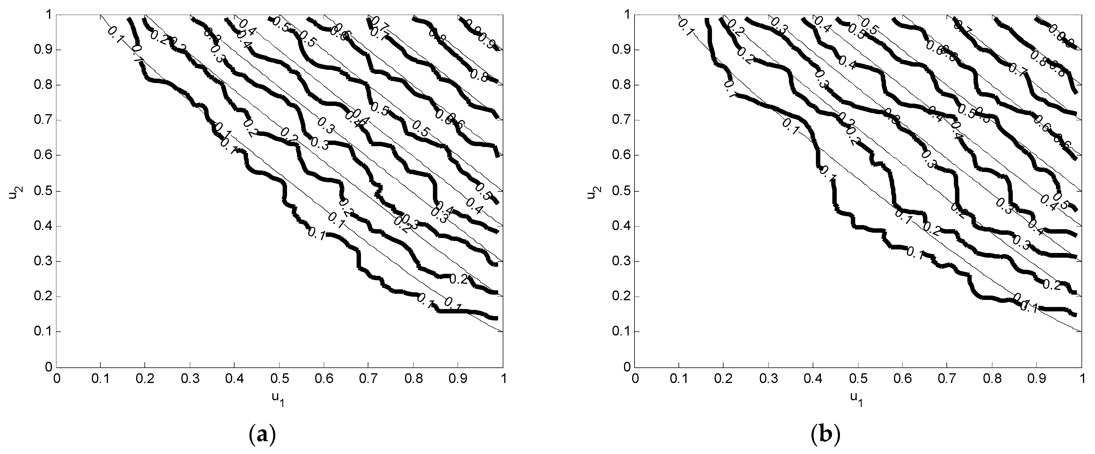
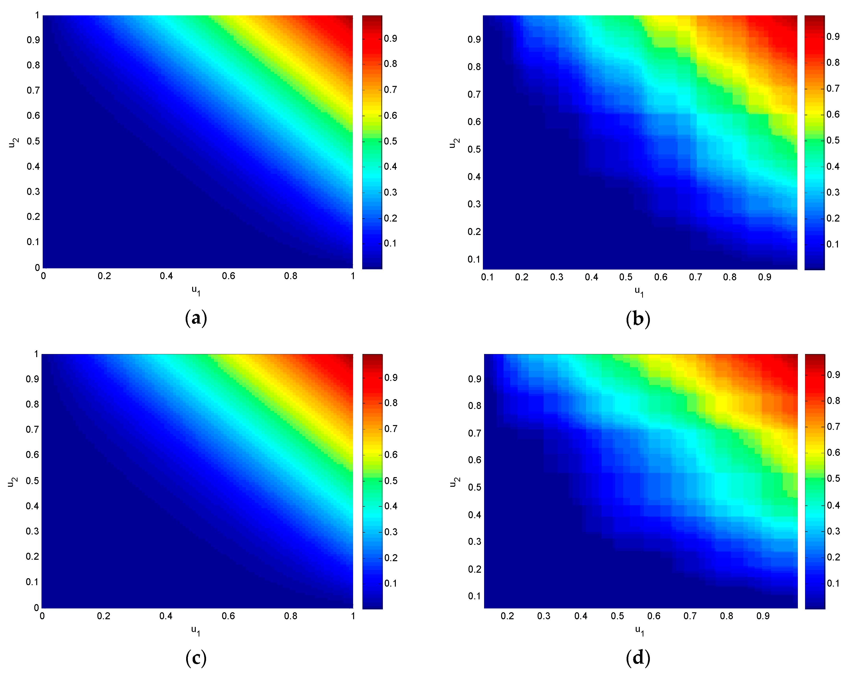
Figure 3 and Figure 4 show the graphical goodness of fit of the selected copula to the empirical data performed for both the analyzed case studies. Empirical data are represented using the empirical (bivariate) copula derived in the form of the discrete function C_n [28] given by:

$$C_n\left(\frac{i}{n},\frac{j}{n}\right)=\frac{\#\left\{\left(x,y\right)|x\le x_{\left(i\right)}andy\le y_{\left(j\right)}\right\}}{n},$$

(10)

where x(i) and y(j), with 1 ≤ i, j ≤ n, denote the order statistics of the sample and # provides the cardinality of the subsequent set.

In particular, Figure 3 shows the contours of the empirical copula (bold lines) plotted together with the theoretical copula (thin lines), while Figure 4 reports the comparison in terms of shaded surfaces.

In both cases, plot analysis confirms how Frank’s copula is adequately fit for modelling the dependence structure between average intensity and rainfall duration.

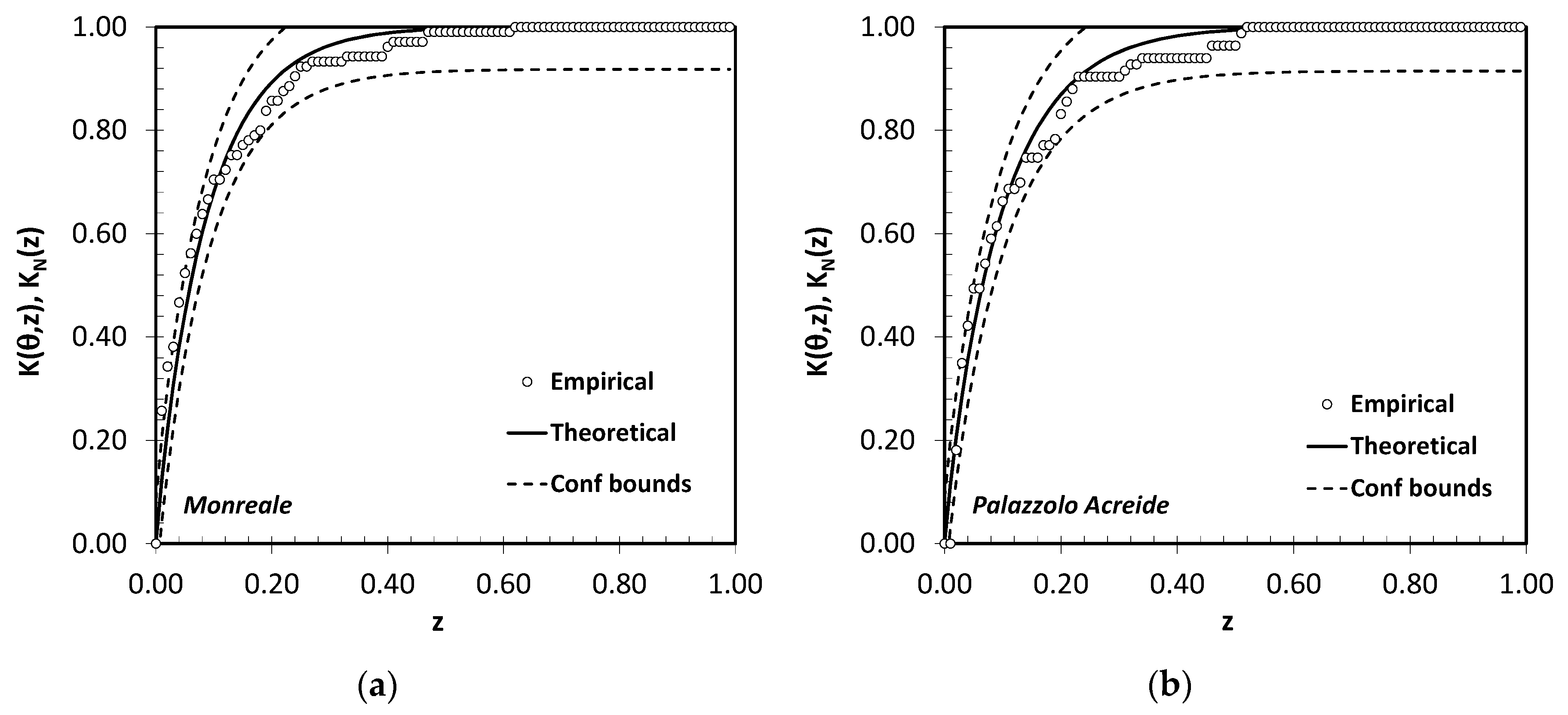
Figure 5, instead, shows the results provided by a further goodness-of-fit graphical procedure proposed by Genest and Rivest [39]. The procedure is based on nonparametric estimates of the distribution function:

$$K\left(\theta ,z\right)=z-\frac{\varphi \left(z\right)}{{\varphi }^{\prime }\left(z\right)}=P\left(C\left(u_1,u_2\right)\le z\right)withzϵ\left(0,1\right],$$

(11)

where u₁ and u₂ denote again realizations of two dependent random variables U₁ and U₂ uniformly distributed between 0 and 1, and C is copula function defined in Equation (2). The empirical nonparametric estimate of K, called K_n, is given by:

$$K_n\left(z\right)=\frac{1}{n}{{\displaystyle \sum }}_{j=1}^{n}1\left(V_{jn}\le z\right)withzϵ\left(0,1\right],$$

(12)

In this equation, 1(A) denote the indicator function of set A (it returns 1 if A is true, 0 if A is false) and V_jn are pseudo-observations defined by:

$$K_n\left(z\right)=\frac{1}{n}{{\displaystyle \sum }}_{k=1}^{n}1\left(X_k\le X_j,Y_k\le Y_j\right)=\frac{1}{n}{{\displaystyle \sum }}_{k=1}^{n}1\left(R_{xk}\le R_{xj},R_{yk}\le R_{yj}\right),$$

(13)

where R_xj and R_yj standing for the rank of X_j and Y_j among X₁,…,X_n and Y₁,…,Y_n.

The graphical comparison reported in Figure 5 between K_n(z) with K(θ,z) shows again the goodness of fit of the empirical data on the theoretical ones.

In the same Figure, the 95% confidence bounds for Frank’s copula are displayed and show how the data are adequately fitted by this kind of copulas. Their limits are calculated in the following form:

$$K_n\left(z\right)\pm \frac{1}{\sqrt{n}}·T_{n,95}$$

(14)

where T_n,95 is the 95% quantile of Kolmogorov–Smirnov statistic T_n [40] under the null hypothesis whose values are equal to 0.747 for Monreale and 0.776 for Palazzolo Acreide respectively.

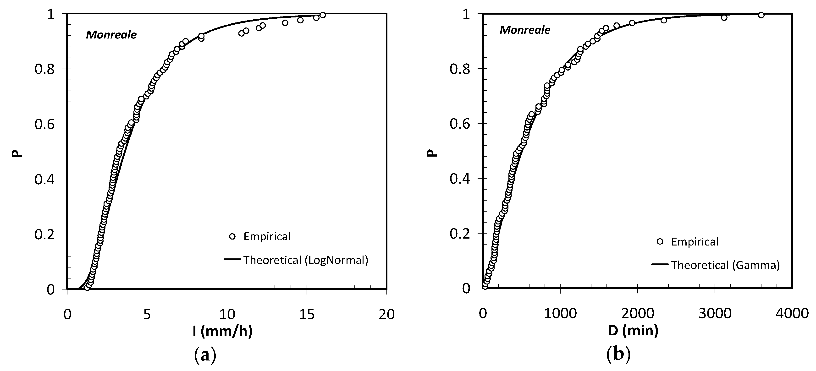
As widely discussed above, copula is able to describe how marginal distributions of two correlated variables are tied together regardless of the scale in which each variable is measured; no assumption is needed for the variables to be independent or have the same type of marginal distributions. Consequently, the other step for the model implementation is the determination of marginal distributions based on univariate data. In the conventional statistical approach, selected intensities (I) and durations (D) values were fitted by several statistical distributions. In particular, Exponential, Gamma, Weibull and Lognormal statistical distributions were considered.

Maximum Likelihood method was applied to define the parameters of these distributions, and the more common statistical tests, as the Akaike Information Criterion (AIC), the Bayesian Information Criterion (BIC), the Relative Root-Mean-Square-Error (RRMSE) and the Chi-Square test [41,42,43] were used to measure the goodness of fit of the analyzed distributions.

Table 3. Marginal distribution parameters and goodness of fit results—Monreale rain gauge station.

Average Intensity	a	b	AIC	BIC	RRMSE	χ2	χ2υ,0.05
Exponential	4.37	-	521.71	524.37	0.62	60.52	28.9
Gamma	2.77	1.58	477.03	482.34	0.32	27.38	27.6
Weibull	4.92	1.58	490.54	495.85	0.38	40.71	27.6
Lognormal	1.28	0.59	461.26	466.57	0.22	20.52	27.6
Duration	a	b	AIC	BIC	RRMSE	χ2	χ2υ,0.05
Exponential	657.14	-	1574.46	1577.11	3.03	30.43	28.87
Gamma	1.36	483.91	1570.91	1576.22	2.34	19.38	27.59
Weibull	695.16	1.16	1572.57	1577.88	2.48	31.19	27.59
Lognormal	6.08	0.98	1572.69	1578.00	4.64	26.24	27.59

and

Table 4. Marginal distribution parameters and goodness of fit results—Palazzolo Acreide rain gauge station.

Average Intensity	a	b	AIC	BIC	RRMSE	χ2	χ2υ,0.05
Exponential	6.38	-	475.55	477.97	0.44	30.93	23.7
Gamma	1.65	3.86	466.64	471.48	0.39	29.39	22.4
Weibull	6.92	1.27	470.20	475.04	0.40	28.61	22.4
Lognormal	1.52	0.82	458.36	463.20	0.34	18.59	22.4
Duration	a	b	AIC	BIC	RRMSE	χ2	χ2υ,0.05
Exponential	775.42	-	1272.47	1274.88	6.64	20.52	23.7
Gamma	0.82	945.80	1272.15	1276.99	4.43	13.58	22.4
Weibull	709.21	0.85	1270.55	1275.39	3.43	23.60	22.4
Lognormal	5.93	1.28	1264.28	1269.12	7.10	9.34	22.4

report the obtained results for both the analyzed case studies, and illustrate how, for both the analyzed sites, Lognormal is the best statistical distribution for describing the rainfall average intensity, whilst Gamma distribution is more suitable for the characterization of the event duration.

Figure 6 shows the two selected individual distributions and the empirical exceedance probabilities of the observed data for the analyzed case studies. In particular, for the i-th observation of a sample of n data, the plotting position was evaluated with the Gringorten equation [41]. This graphical analysis demonstrates how the empirical data are well represented by the chosen statistical distributions.

2.5. Generation of Rainfall Event Profile

For the complete characterization of an event, once the main storm characteristics are generated, it is necessary to establish the rainfall event profile. To this aim, the concept of mass curves, defined as normalized cumulative storm depth versus normalized time since the beginning of a storm, extensively applied by several authors [11,13,44], has been utilized. According to this theory, for an event of total duration D, average rainfall intensity I and, consequently, cumulative storm volume V = I·D, its pattern is represented by a dimensionless rainfall hyetograph defined as:

$$H\left(d\right)=\frac{1}{V}{{\displaystyle \int }}_0^{t}h\left(t\right)dt,$$

(15)

where t (0 ≤ t ≤ D) is the considered time interval of the event divided by the total duration and, consequently, d = t/D (0 ≤ d ≤ 1) is the correspondent dimensionless duration; h(t) is the fraction of the total rainfall depth of the analyzed event at time t (0 ≤ h ≤ V) and, consequently, H = H(d)/V is the correspondent dimensionless rainfall depth.

The choice of an appropriate time step in which each rainfall event has to be divided into is a fundamental step in creating reliable dimensionless hyetographs. This value needs to be adequately fixed in order to guarantee the preservation of the event characteristics to this end, taking into account of the time-resolution of the data available for the creation of these dimensionless curves, a time interval equal to 10 min was fixed.

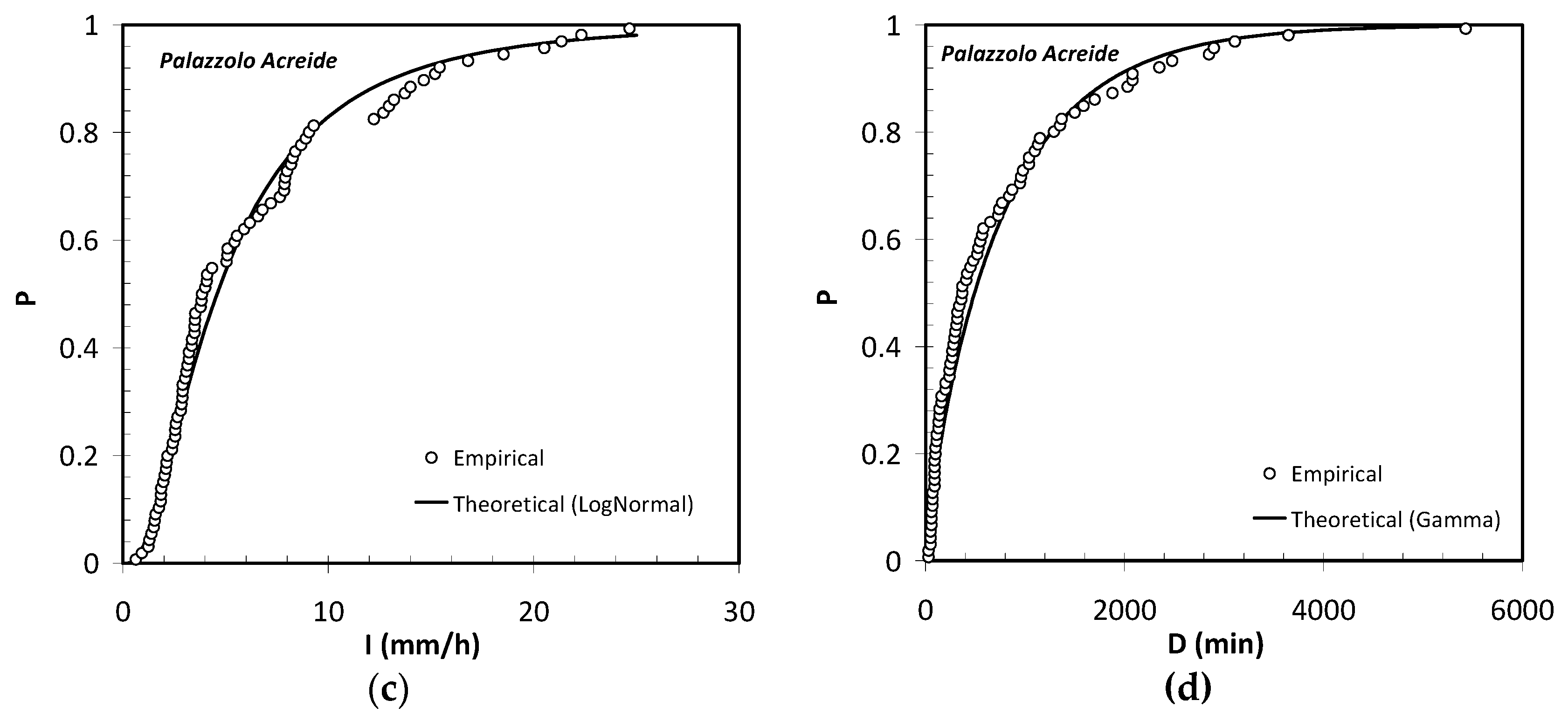
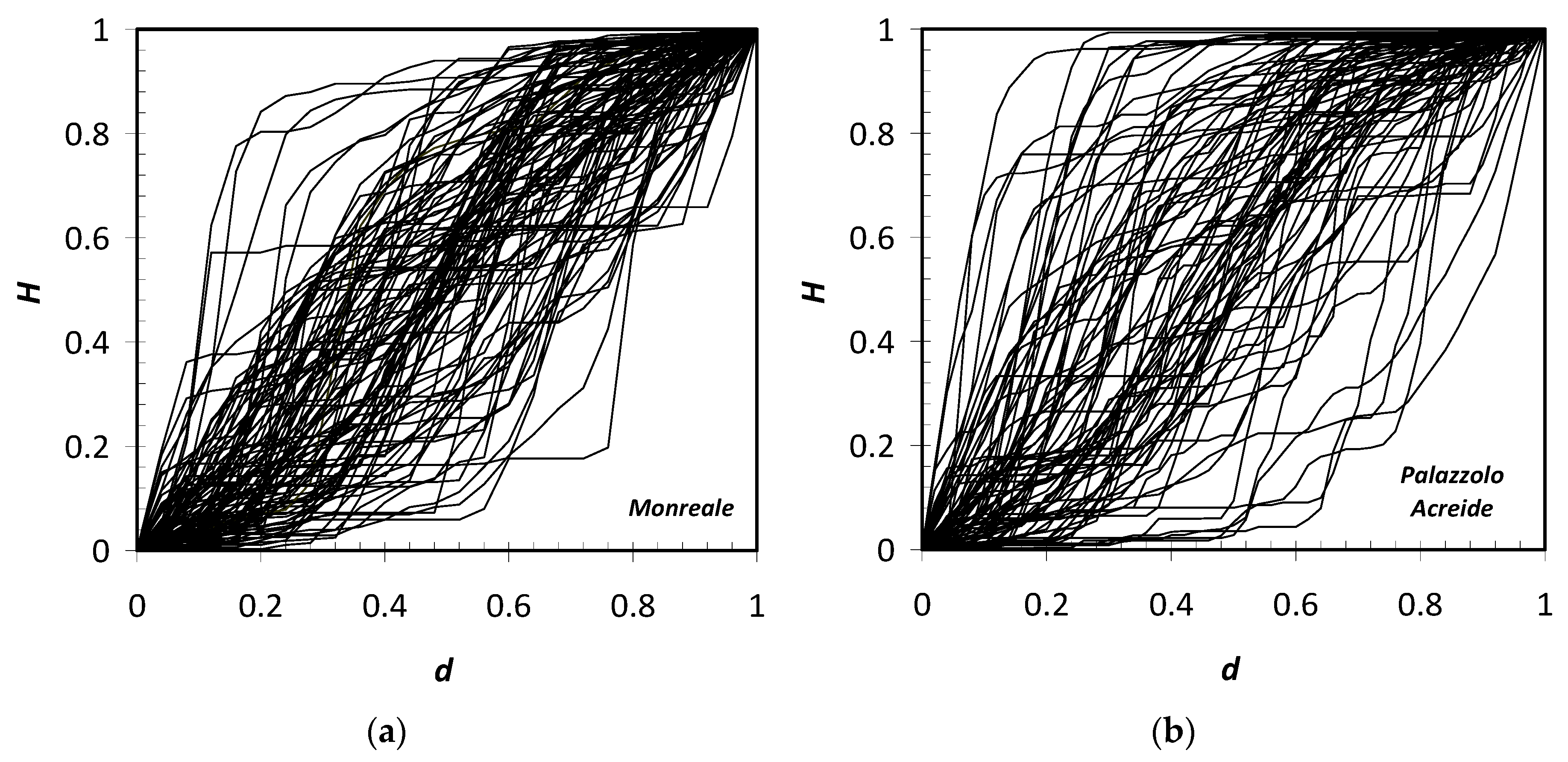
Dimensionless hyetographs thus derived for the selected rainfall events and for both the considered rain gauge stations are plotted in Figure 7.

These empirical curves have been used for calibrating the stochastic model of the rainfall event profile. Following the Garcia-Guzman and Aranda-Oliver approach [13], for modelling event profiles, Beta cumulative distribution was adopted, for each considered time-step. How outlined by several authors [1,13], in fact, the fixed upper and lower bounds of this statistical distribution and its particular shape density function make it able to adequately fits this kind of data and, hence, particularly suitable for this modelling.

The probability density function of the Beta distribution is a power function of the variable x and of its reflection (1-x) defined as:

$$f(x|\alpha ,\beta )=\frac{1}{B\left(\alpha ,\beta \right)}{x}^{\alpha -1}{(1-x)}^{\beta -1}for0\le x\le 1,$$

(16)

where B(α,β) is the Beta function with shape positive parameters α and β given by:

$$B\left(\alpha ,\beta \right)=\frac{\mathsf{\Gamma }\left(\alpha +\beta \right)}{\mathsf{\Gamma }\left(\alpha \right)\mathsf{\Gamma }\left(\beta \right)},$$

(17)

and Γ corresponds to the Gamma function.

The cumulative Beta distribution function is defined, instead, as:

$$F\left(x|\alpha ,\beta \right)=\frac{B\left(x|\alpha ,\beta \right)}{B\left(\alpha ,\beta \right)}=\frac{1}{B\left(\alpha ,\beta \right)}{{\displaystyle \int }}_0^x{t}^{\alpha -1}{\left(1-t\right)}^{\beta -1}dt,$$

(18)

To overcome the limitation due to the different number of time-steps in which each rainfall event has been divided into and to preserve rainfall characteristics, historical normalized mass curves have been sampled in 26 equal time-steps (0; 0.04; 0.08; …; 0.96; 1). This number was chosen in order to avoid time-steps lower than 10 min. For each time-step, parameters of the Beta cumulative distribution have been estimated by using the method of maximum likelihood and values thus obtained are shown in

Table 5. Beta distribution parameters for different normalized time-step.

Monreale
d	0.04	0.08	0.12	0.16	0.20	0.24	0.28	0.32	0.36	0.40	0.44	0.48
α	1.113	1.120	1.070	1.070	1.185	1.296	1.410	1.622	1.869	2.079	2.214	2.327
β	30.562	15.247	8.741	6.029	4.938	4.057	3.474	3.218	3.032	2.805	2.509	2.227
d	0.52	0.56	0.6	0.64	0.68	0.72	0.76	0.8	0.84	0.88	0.92	0.96
α	2.585	2.940	3.468	4.028	4.435	5.097	5.879	8.219	10.976	13.691	19.830	45.558
β	2.068	1.931	1.790	1.648	1.447	1.363	1.276	1.330	1.309	1.187	1.080	1.121
Palazzolo Acreide
d	0.04	0.08	0.12	0.16	0.20	0.24	0.28	0.32	0.36	0.40	0.44	0.48
α	0.792	0.749	0.737	0.778	0.789	0.830	0.877	0.955	1.035	1.150	1.243	1.344
β	16.766	7.010	4.063	3.001	2.290	1.845	1.515	1.301	1.158	1.072	1.000	0.934
d	0.52	0.56	0.6	0.64	0.68	0.72	0.76	0.8	0.84	0.88	0.92	0.96
α	1.616	1.922	2.111	2.440	3.225	3.681	4.456	5.884	9.340	12.947	21.020	54.655
β	0.931	0.905	0.814	0.754	0.770	0.730	0.734	0.765	0.843	0.846	0.842	0.970

.

3. Results

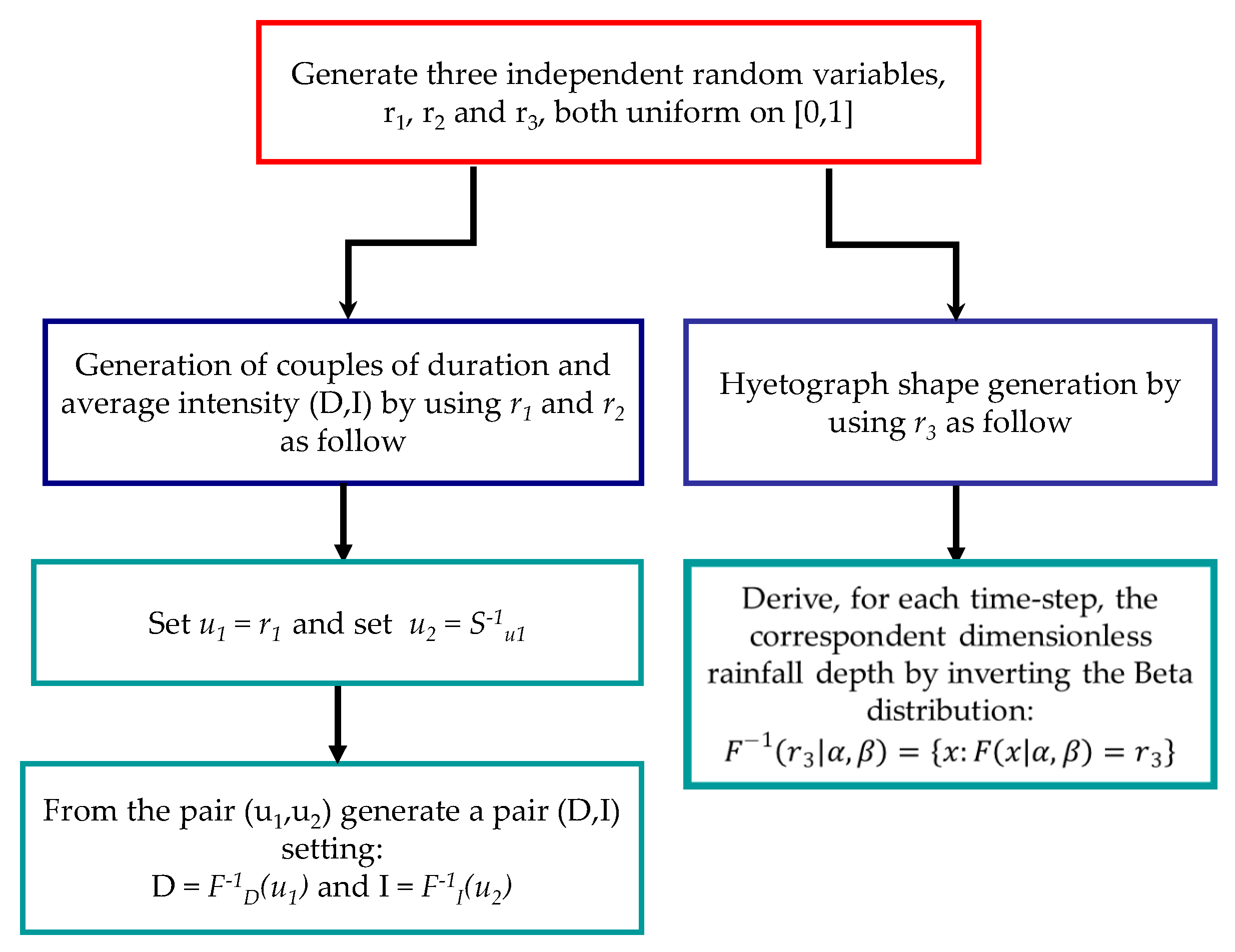
For the implementation of the methodology, 20,000 single storm events were generated for each analyzed site using the Monte Carlo procedure represented in Figure 8 and described below. The number of simulations was chosen to guarantee the balance of the require degree of accuracy and the computational effort necessary [45].

For each i-th simulation (with 1 < i < 20,000), the model firstly generates the event’s main characteristics (storm duration D_i and rainfall average intensity I_i) by using Frank’s copula, then define its temporal pattern by applying the Beta distribution with parameter α and β estimated, for each time step, on the basis of the observed rainfall patterns.

Going into more details, Monte Carlo generation of pairs of storm duration and average rainfall intensity (D, I) can be easily carried out by applying the algorithm proposed by Nelsen [38,46]. Following this procedure, the code initially creates two independent random variables, called r₁ and r₂, both uniform on [0,1]. Starting from these two variables, the code derives two new parameters, called u₁ and u₂, setting $u_1=r_1$ and $u_2=S_{u_1}^{-1}\left(r_2\right)$ where $S_{u_1}\left(r_2\right)$ is a function which exists and is non-decreasing almost everywhere in [0,1] defined as:

$$S_{u_1}\left(r_2\right)=\frac{\partial C\left(u_1,u_2\right)}{\partial u_1}=Pr\left\{U_2\le u_2|U_1=u_1\right\},$$

(19)

where C(u₁,u₂) is the Frank’s copula defined by Equation (7).

The pair (D, I) is then generated from the pair (u₁, u₂) through the inversion of the marginal distributions of storm duration and rainfall average intensity previously determined, setting:

$$D=F_D^{-1}\left(u_1\right)\mathrm{and}I=F_I^{-1}\left(u_2\right),$$

(20)

Once that the pair (D, I) has been defined, in order to create a synthetic event, the code performs the generation of a synthetic dimensionless hyetograph.

This can be easily carried out by randomly generating a new variable r₃, uniform distributed on [0,1], and calculating the dimensionless hyetograph by inverting Equation (18) as follow:

$$F^{-1}\left(r_3|\alpha ,\beta \right)=\left\{x:F\left(x|\alpha ,\beta \right)=r_3\right\},$$

(21)

Equation (21) provides, for given pair of parameters α and β estimated for each considered time-step, the values of the correspondent dimensionless rainfall depth. Finally, with Equation (15) we are able to obtain of the final hyetograph.

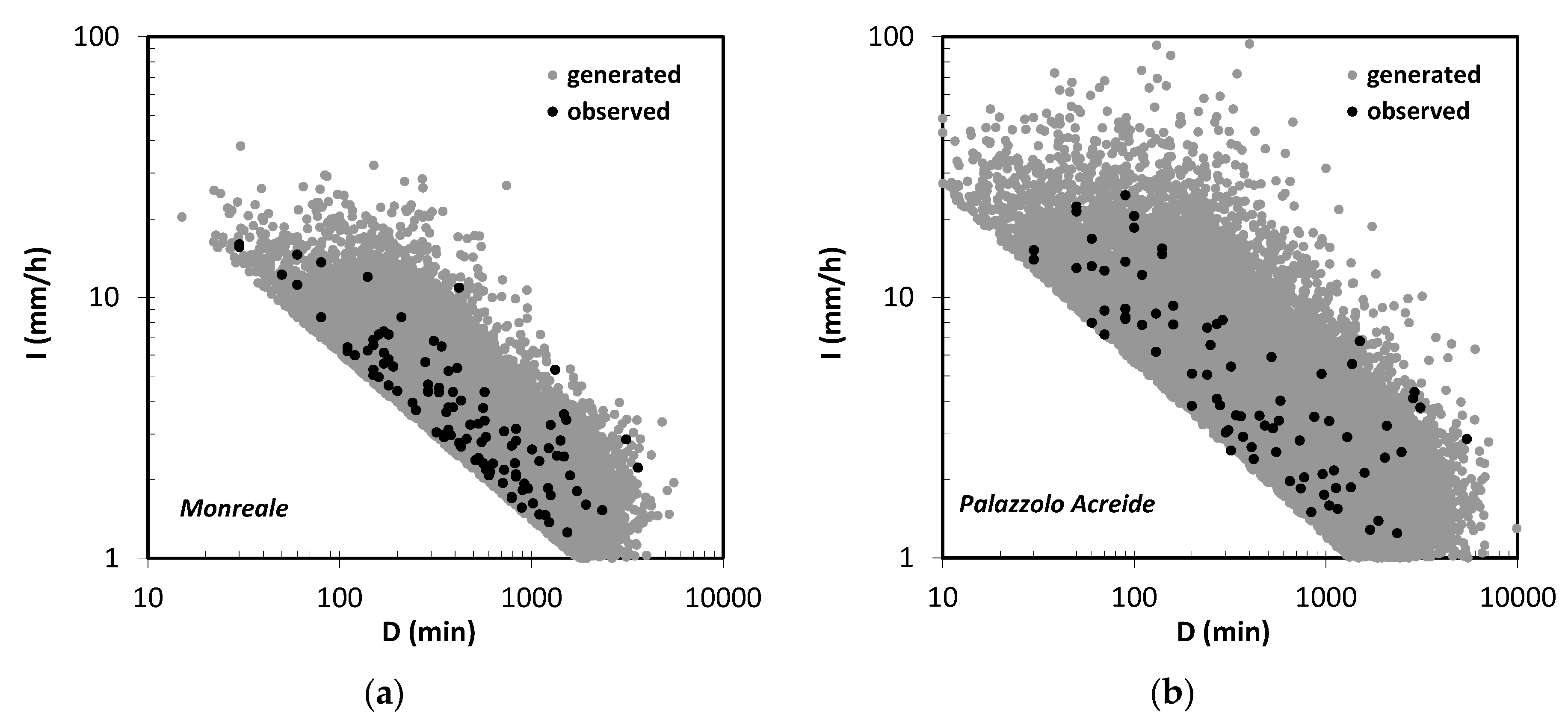
The events so generated have been compared with the observed ones and the obtained results are represented in Figure 9 and Figure 10. More in detail, Figure 9 shows the comparison between the correlation structure of generated and observed events and demonstrate how the duration-intensity correlation of the generated couples is congruent with that one of the observed couples.

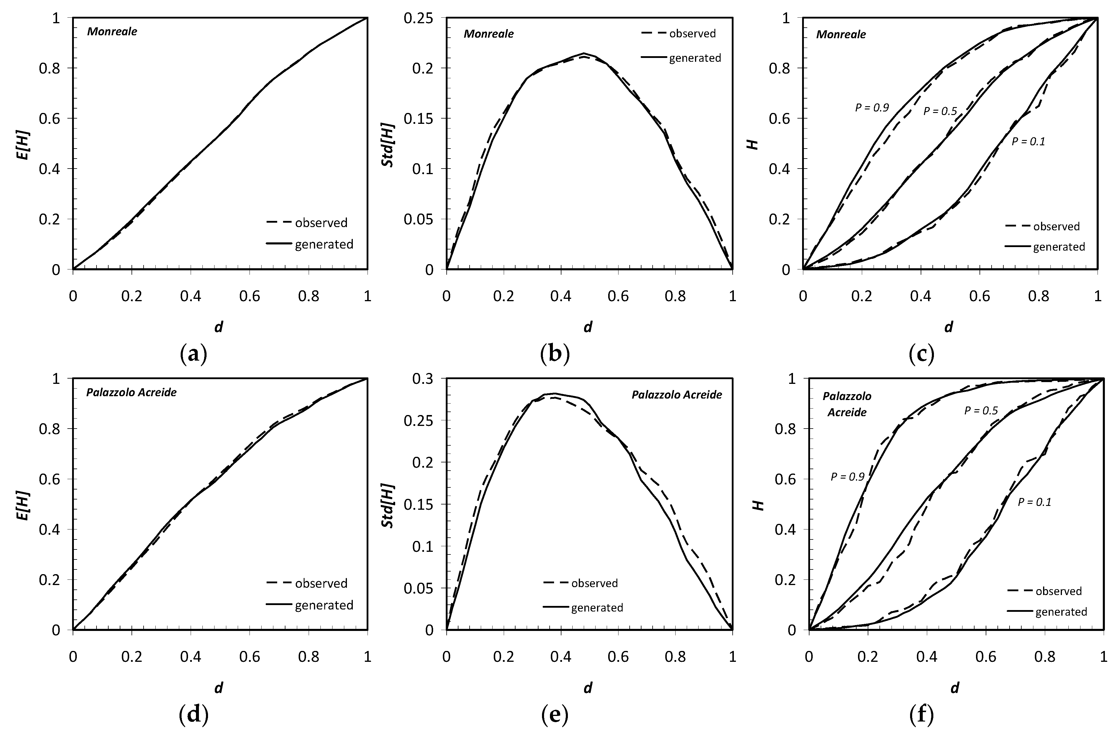
In Figure 10, the main statistics of observed and generated hyetograph shape are plotted. In particular mean, standard deviation and 10th, 50th and 90th percentiles derived, for each considered time-step, both for the generated hyetographs and for the observed ones have been overlapped for each analyzed case study, demonstrating a very good capacity of the model to reproduce these statistics.

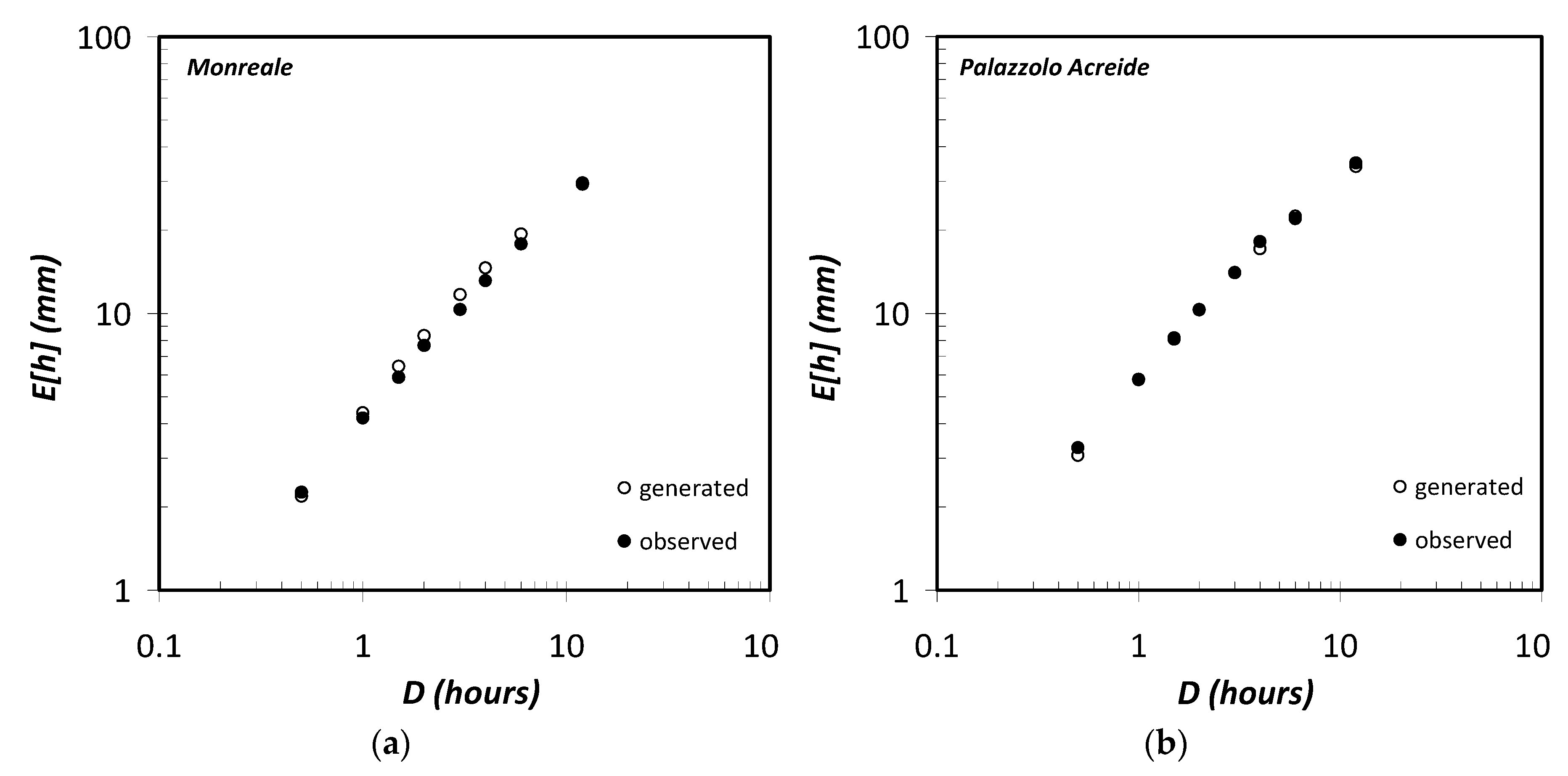
Finally, Figure 11 reports the comparison between the expected values of the maximum depth for fixed duration calculated for both series (generated and observed), showing again very satisfying results.

4. Discussions and Conclusions

A stochastic rainfall model for simulating synthetic sub-hourly rainfall events at a given site has been presented. Taking into account the statistical correlation between the main event characteristics, the Archimedean copula family, and in particular the Frank’s copula, was implemented. For both the analyzed case studies, the statistical tests performed suggested that the Lognormal is the best statistical distribution for characterizing the rainfall average intensity and the Gamma statistical distribution is more suitable to describe the event duration.

In order to describe the temporal pattern of the rainfall within each generated event, all the historical dimensionless events, sampled in several time-steps, were statistically analyzed by applying the Beta distribution. Although other cumulative distribution functions could be used for modelling the dimensionless rainfall at individual time-steps, as for example the Kumarasawamy statistical distribution, the Beta distribution was selected in this application because of its capacity to reproduce well this kind of data. Beta distribution was applied for each sample derived for each considered time-step and the correspondent shape parameters were estimated. In this way, it was possible to obtain the statistical parameters for each considered time-step that made it possible to derive rainfall profile for a given generated event. Once that dimensionless rain process is fully characterized, only the total amount of precipitation and the storm duration have to be inserted in order to get an event.

The results are plotted in Figure 9, Figure 10 and Figure 11 and the good agreement between the statistics of observed and derived rainfall events, for both the analyzed case studies, is a robust indicator of the good performance of the model. Figure 9 and Figure 10 demonstrate, in fact, how the synthetic events so generated reproduce reasonably well the statistics of the historic observed events, both with regard to the duration-intensity correlation (Figure 9), and also with regard to their temporal pattern (Figure 10).

In particular, the results showed in Figure 9 confirm how the statistical dependence between storm duration and rainfall intensity can be adequately modelled by applying the Frank’s copula and how the selected marginal distributions, for each considered variable, allow their correlation structure to be well respected.

For what concerns the generator’s capacity to reproduce the temporal pattern of the rainfall, looking at Figure 10c,f, where the 10th, 50th and 90th percentiles of the hyetograph shape are plotted, it is possible to verify how the generated curves have nonlinear shape in accordance with the observed ones. Moreover, all the curves plotted in Figure 10 show how generated and observed values at each step are very close to each other without any remarkable deviation, except, perhaps for the standard deviation comparison where, in some points, a little discrepancy can be observed. The good results obtained provide a good indicator of how the temporal pattern sub-model make it possible to effectively represent the statistical characteristics of the observed event shape.

More significant for the aim of the present study are the results shown in Figure 11. In those graphs, the comparison between mean of the rainfall depth for fixed duration, both for observed and for generated events, was plotted. The good agreement between historic and generated points is a significant indicator of the capability and the robustness of the proposed model to generate meaningfully extreme rainfall events as well. In addition, it is worth to pointing out that there is good agreement for the short and for the longer durations, which is in accordance with one of the main purposes of this methodology.

Hence, the model is capable to easily generate a long sequence of sub-hourly synthetic rainfall events consistent with the main hydrological characteristics of a considered site.

Because of its simplicity and of the limited data necessary for its calibration, the model could be very useful in those sites where long recorded and high-resolution rainfall series are not always available. Dealing with few years of rainfall data series is not possible to work with the annual maxima. This implies the need of selecting, for each considered year, significant events to perform the calculation. This selection has been in this study linked to the average annual number of significant rainfall episodes. This selection should ensure to deal with independent events that can be considered as hydrologically “significant” for the possible formation of a flooding.

Conversely, a limitation of the methodology lies in the historic event selection. Dealing with few years of high-resolution rainfall series, is not possible perform a robust statistical analysis by selecting only the annual maxima. This implies the need to select more events for year that have to be independent of each other and hydrologically significant. For this aim, the procedure proposed by Rahman et al. was in study followed. Exclusion of low intensity rainfall reduces the data domain to the interval (int_min, infty). However, in order to preserve the simplicity of the model we decided to use the non-truncated marginal distributions (only 2 parameters instead of 3 each) and, instead, preferred to reduce the domain of the generated data by using the same truncation threshold. Of course, the availability of longer rainfall series characterized by high temporal resolution could make it possible to overcome this limitation, as it could be possible to work only with annual maxima.

Furthermore, the model assumes as a hypothesis that the data used for the analysis are stationary. This hypothesis can reasonably be considered valid, given the limited number of the years considered. Moreover, some studies in Sicily [47,48] have shown how for all the time series analyzed, no trend actually exists, and consequently, they denote a stationary behavior.

References

- Acreman, M.C. A simple stochastic model of hourly rainfall for Farnborough, England. Hydrol. Sci. J. 1990, 35, 119–148. [Google Scholar] [CrossRef] [Green Version]
- Cameron, D.; Beven, K.; Tawn, J. An evaluation of three stochastic rainfall models. J. Hydrol. 2000, 228, 130–149. [Google Scholar] [CrossRef]
- Mendoza-Resendiz, A.; Arganis-Juarez, M.; Dominguez-Mora, R.; Echavarria, B. Method for generating spatial and temporal synthetic hourly rainfall in the Valley of Mexico. Atmos. Res. 2013, 132–133, 411–422. [Google Scholar] [CrossRef]
- Bonaccorso, B.; Brigandì, G.; Aronica, G.T. Combining regional rainfall frequency analysis and rainfall-runoff modelling to derive frequency distributions of peak flows in ungauged basins: A proposal for Sicily region (Italy). Adv. Geosci. 2017, 44, 15–22. [Google Scholar] [CrossRef]
- Cowpertwait, P.S.P.; O’Connell, P.E.; Metcalfe, A.V.; Mawdsley, J.A. Stochastic point process modelling of rainfall. I. Single-site fitting and validation. J. Hydrol. 1996, 175, 17–46. [Google Scholar] [CrossRef]
- Cowpertwait, P.S.P.; O’Connell, P.E.; Metcalfe, A.V.; Mawdsley, J.A. Stochastic point process modelling of rainfall. II. Regionalisation and disaggregation. J. Hydrol. 1996, 175, 47–65. [Google Scholar] [CrossRef]
- Blazkova, S.; Beven, K.J. Flood frequency prediction for data limited catchments in the Czech Republic using a stochastic rainfall model and TOPMODEL. J. Hydrol. 1997, 195, 256–278. [Google Scholar] [CrossRef]
- Koutsoyiannis, D.; Mamassis, N. On the representation of hyetograph characteristics by stochastic rainfall models. J. Hydrol. 2001, 251, 65–87. [Google Scholar] [CrossRef]
- Candela, A.; Brigandì, G.; Aronica, G.T. Estimation of synthetic flood design hydrographs using a distributed rainfall-runoff model coupled with a copula-based single storm rainfall generator. Nat. Hazards Earth Syst. Sci. 2014, 14, 1819–1833. [Google Scholar] [CrossRef]
- Gao, C.; Xu, Y.P.; Zhu, Q.; Bai, Z.; Liu, L. Stochastic generation of daily rainfall events: A single-site rainfall model with Copula-based joint simulation of rainfall characteristics and classification and simulation of rainfall patterns. J. Hydrol. 2018, 564, 41–58. [Google Scholar] [CrossRef]
- Huff, F. Time Distribution Rainfall in Heavy Storms. Water Resour. Res. 1967, 3, 1007–1019. [Google Scholar] [CrossRef]
- Eagleson, P.S. Dynamics of flood frequency. Water Resour. Res. 1972, 8, 878–898. [Google Scholar] [CrossRef]
- Garcia-Guzman, A.; Aranda-Oliver, E. A Stochastic model of dimensionless hyetograph. Water Resour. Res. 1993, 29, 2363–2370. [Google Scholar] [CrossRef]
- Robinson, J.S.; Silvapalan, M. Temporal scales and hydrological regimes: Implications for flood frequency scaling. Water Resour. Res. 1997, 33, 2981–2999. [Google Scholar] [CrossRef] [Green Version]
- Rodriguez-Iturbe, I.; Febres de Power, B.; Valdes, J.B. Rectangular pulses point process models for rainfall: Analysis of empirical data. J. Geophys. Res. 1987, 92, 9645–9656. [Google Scholar] [CrossRef]
- Calenda, G.; Napolitano, F. Parameter estimation of Neyman-Scott processes for temporal point rainfall simulation. J. Hydrol. 1999, 225, 45–66. [Google Scholar] [CrossRef]
- Onof, C.; Wheater, H.S. Modelling of British rainfall using a random parameter Bartlett–Lewis rectangular pulse model. J. Hydrol. 1993, 149, 67–95. [Google Scholar] [CrossRef]
- Onof, C.; Wheater, H.S. Improvements to the modelling of British rainfall using a modified random parameter Bartlett–Lewis rectangular pulse model. J. Hydrol. 1994, 157, 177–195. [Google Scholar] [CrossRef]
- Onof, C.; Wheater, H.S. Improved fitting of the Bartlett–Lewis rectangular pulse model for hourly rainfall. Hydrol. Sci. J. 1994, 39, 663–680. [Google Scholar] [CrossRef]
- Khaliq, M.N.; Cunnane, C. Modelling point rainfall occurrences with the modified Bartlett-Lewis Rectangular Pulses Model. J. Hydrol. 1996, 180, 109–138. [Google Scholar] [CrossRef]
- Koutsoyiannis, D.; Foufoula-Georgiou, E. A scaling model of a storm hyetograph. Water Resour. Res. 1993, 29, 2345–2361. [Google Scholar] [CrossRef]
- Heneker, T.M.; Lambert, M.F.; Kuczera, G. A point rainfall model for risk-based design. J. Hydrol. 2001, 247, 54–71. [Google Scholar] [CrossRef]
- Córdova, J.R.; Rodríguez-Iturbe, I. On the probabilistic structure of storm surface runoff. Water Resour. Res. 1985, 21, 755–763. [Google Scholar] [CrossRef]
- Singh, K.; Singh, V.P. Derivation of bivariate probability density functions with exponential margins. Stoch. Hydrol. Hydraul. 1991, 5, 55–687. [Google Scholar] [CrossRef]
- Bacchi, B.; Becciu, G.; Kottegoda, N.T. Bivariate exponential model applied to intensities and duration of extreme rainfall. J. Hydrol. 1994, 155, 225–236. [Google Scholar] [CrossRef]
- Kurothe, R.S.; Goel, N.K.; Mathur, B.S. Derived flood frequency distribution for negatively correlated rainfall intensity and duration. Water Resour. Res. 1997, 33, 2103–2107. [Google Scholar] [CrossRef] [Green Version]
- De Michele, C.; Salvadori, G. A Generalized Pareto intensity-duration model of storm rainfall exploiting 2-Copulas. J. Geophys. Res. 2003, 108, 4067. [Google Scholar] [CrossRef]
- Zhang, L.; Singh, V.P. Bivariate rainfall frequency distributions using Archimedean copulas. J. Hydrol. 2006, 332, 93–109. [Google Scholar] [CrossRef]
- Salvadori, G.; De Michele, C.; Kottegoda, N.T.; Rosso, R. Extremes in Nature. An Approach Using Copulas; Springer: Berlin, Germany, 2007. [Google Scholar]
- Favre, A.C.; El Adlouni, S.; Perreault, L.; Thiémonge, N.; Bobée, B. Multivariate hydrological frequency analysis using copulas. Water Resour. Res. 2004, 40, 1–12. [Google Scholar] [CrossRef]
- Salvadori, G.; De Michele, C. Frequency analysis via copulas: Theoretical aspects and applications to hydrological events. Water Resour. Res. 2004, 40, 1–17. [Google Scholar] [CrossRef]
- Genest, C.; Favre, A.C. Everything you always wanted to know about copula modeling but were afraid to ask. J. Hydrol. Eng. ASCE 2007, 12, 347–368. [Google Scholar] [CrossRef]
- Cantet, P.; Arnaud, P. Extreme rainfall analysis by a stochastic model: Impact of the copula choice on the sub-daily rainfall generation. Stoch. Environ. Res. Risk Assess. 2014, 28, 1479–1492. [Google Scholar] [CrossRef]
- Vandenberghe, S.; Verhoest, N.E.C.; Buyse, E.; De Baets, B. A stochastic design rainfall generator based on copulas and mass curves. Hydrol. Earth. Syst. Sci. 2010, 14, 2429–2442. [Google Scholar] [CrossRef] [Green Version]
- Cannarozzo, M.; D’asaro, F.; Ferro, V. Regional rainfall and flood frequency analysis for Sicily using the two component extreme value distribution. Hydrol. Sci. J. 1995, 40, 19–42. [Google Scholar] [CrossRef] [Green Version]
- Rahman, A.; Weinmann, P.E.; Hoang, T.M.T.; Laurenson, E.M. Monte Carlo simulation of flood frequency curves from rainfall. J. Hydrol. 2002, 256, 196–210. [Google Scholar] [CrossRef]
- Rossi, F.; Fiorentino, M.; Versace, P. Two-Component Extreme Value Distribution for Flood Frequency Analysis. Water Resour. Res. 1984, 20, 847–856. [Google Scholar] [CrossRef]
- Nelsen, R.B. An Introduction to Copulas. Lecture Notes in Statistics; Springer: New York, NY, USA, 1999. [Google Scholar]
- Genest, C.; Rivest, L. Statistical inference procedures for bivariate Archimedean copulas. J. Am. Stat. Assoc. 1993, 88, 1034–1043. [Google Scholar] [CrossRef]
- Genest, C.; Quessy, J.F.; Remillard, B. Goodness-of-fit Procedures for Copula Models Based on the Probability Integral Transformation. Scand. J. Stat. 2006, 33, 337–366. [Google Scholar] [CrossRef]
- Chow, V.T.; Maidment, D.R.; Mays, L.W. Applied Hydrology; McGraw-Hill International: New York, NY, USA, 1998. [Google Scholar]
- Maidment, D.R. Handbook of Hydrology; McGraw-Hill International: New York, NY, USA, 1992. [Google Scholar]
- Kottegoda, N.T.; Rosso, R. Applied Statistics for Civil and Environmental Engineers; Blackwell Publishing Ltd.: Oxford, UK, 2008. [Google Scholar]
- Salvadori, G.; De Michele, C. Statistical characterization of temporal structure of storms. Adv. Water Res. 2006, 29, 827–842. [Google Scholar] [CrossRef]
- Aronica, G.T.; Candela, A. Derivation of flood frequency curves in poorly gauged catchments using a simple stochastic hydrological rainfall-runoff model. J. Hydrol. 2007, 347, 132–142. [Google Scholar] [CrossRef]
- De Michele, C.; Salvadori, G.; Canossi, M.; Petaccia, A.; Rosso, R. Bivariate Statistical Approach to Check Adequacy of Dam Spillway. J. Hydrol. Eng. ASCE 2005, 10, 50–57. [Google Scholar] [CrossRef]
- Bonaccorso, B.; Aronica, G.T. Estimating Temporal Changes in Extreme Rainfall in Sicily Region (Italy). Water Resour. Manag. 2016, 30, 5651–5670. [Google Scholar] [CrossRef]
- Arnone, E.; Pumo, D.; Viola, F.; Noto, L.V.; La Loggia, G. Rainfall statistics changes in Sicily. Hydrol. Earth Syst. Sci. 2013, 17, 2449–2458. [Google Scholar] [CrossRef] [Green Version]
Figure 1.
Location of the rain gauge stations used for the study.
Figure 2.
Events selected for the study with the threshold curve at: (a) Monreale; (b) Palazzolo Acreide.
Figure 3.
Contour plotting of empirical vs. theoretical copula at: (a) Monreale; (b) Palazzolo Acreide.
Figure 4.
Shaded surfaces of empirical ((b,d)) vs. theoretical copula ((a,c)) at: Monreale ((a,b)); Palazzolo Acreide ((c,d)).
Figure 5.
Comparison of K(z) values for Frank copula with empirical data: (a) Monreale; (b) Palazzolo Acreide.
Figure 6.
Plotting position: (a) average intensity at Monreale; (b) duration at Monreale; (c) average intensity at Palazzolo Acreide; (d) duration at Palazzolo Acreide.
Figure 7.
Dimensionless hyetographs for the selected events at: (a) Monreale; (b) Palazzolo Acreide.
Figure 8.
Flow diagram of the Monte Carlo simulation.
Figure 9.
Comparison between 20.000 values generated from the Frank’s copulas fitted on the observed data and observed events at: (a) Monreale; (b) Palazzolo Acreide.
Figure 10.
Comparison between observed and generated hyetograph shape: (a) mean at the Monreale rain gauge station; (b) standard deviation at the Monreale rain gauge station; (c) 10th, 50th and 90th at the Monreale rain gauge station; (d) mean at the Palazzolo Acreide rain gauge station; (e) standard deviation at the Palazzolo Acreide rain gauge station; (f) 10th, 50th and 90th at the Palazzolo Acreide rain gauge station.
Figure 11.
Comparison between observed and generated events—mean of the maximum depth for fixed duration: (a) Monreale; (b) Palazzolo Acreide.