Article

Geophysical and Sedimentological Investigations of Peatlands for the Assessment of Lithology and Subsurface Water Pathways

Institute of Geography and Geology, Department of Physical Geography, University Wuerzburg, Am Hubland, 97074 Würzburg, Germany
*
Author to whom correspondence should be addressed.
Geosciences 2019, 9(3), 118; https://doi.org/10.3390/geosciences9030118
Submission received: 30 December 2018 / Revised: 29 January 2019 / Accepted: 1 February 2019 / Published: 8 March 2019

Abstract

:
Peatlands located on slopes (herein called slope bogs) are typical landscape units in the Hunsrueck, a low mountain range in Southwestern Germany. The pathways of the water feeding the slope bogs have not yet been documented and analyzed. The identification of the different mechanisms allowing these peatlands to originate and survive requires a better understanding of the subsurface lithology and hydrogeology. Hence, we applied a multi-method approach to two case study sites in order to characterize the subsurface lithology and to image the variable spatio-temporal hydrological conditions. The combination of Electrical Resistivity Tomography (ERT) and an ERT-Monitoring and Ground Penetrating Radar (GPR), in conjunction with direct methods and data (borehole drilling and meteorological data), allowed us to gain deeper insights into the subsurface characteristics and dynamics of the peatlands and their catchment area. The precipitation influences the hydrology of the peatlands as well as the interflow in the subsurface. Especially, the geoelectrical monitoring data, in combination with the precipitation and temperature data, indicate that there are several forces driving the hydrology and hydrogeology of the peatlands. While the water content of the uppermost layers changes with the weather conditions, the bottom layer seems to be more stable and changes to a lesser extent. At the selected case study sites, small differences in subsurface properties can have a huge impact on the subsurface hydrogeology and the water paths. Based on the collected data, conceptual models have been deduced for the two case study sites.

1. Introduction

Peatlands located on slopes (herein called slope bogs) are typical landscape units in the Hunsrueck, a low mountain range in Southwestern Germany, and have often been drained since the early 19th century to grow spruce (Picea abies) in the development of forests [1]. These peatlands are mainly fed from downslope interflow, direct precipitation and groundwater springs. In addition to high precipitation, including snow, fog was also seen as an important factor in the feeding of these peatlands with moisture [2].
The influence of ditches for the drainage of the peatlands is already well documented in the Hunsrueck, with a focus especially on the output and water capacity of the ditches [3]. Additional pedological or phenological research has been conducted in the study area [1,4,5]. These studies touch the topic of the hydrology of the peatlands, with a focus on springs and the water flow within them, but the pathways of the water feeding the slope bogs have not yet been documented and analyzed. By contrast, the hydrology of many different types of mires, bogs and peatlands worldwide is less complex and well-described [6]. Studies more often focus on more specific questions, such as carbon dioxide storage capacity [7,8]. However, especially the mosses within the wet parts of the peatland are of great significance for nature conservation and protection [4] and the slope bogs within the area of investigation have been identified as priority conservation. A 30-year plan for renaturation and restoration that mainly concentrates on the slope bogs has started, since the founding of the national park, Hunsrueck–Hochwald, in 2015 [3].
Due to the difference in resistivity between dry rocks, wet rocks, sediments and organic matter; Electrical Resistivity Tomography (ERT) is an adequate method for identifying not only subsurface lithology, but also near-surface water paths within peatlands and their catchment areas. Some studies by North American scientists investigated different types of peatlands, e.g., esker deposits and pool systems below peat [9], carbon storage of tropical peatlands in Indonesia [6] or the resistivity-based monitoring of biogenic gases in peat soils [10]. In Europe [11], studies on the internal structure of alpine mires with ERT [12] tried to distinguish alpine bogs and fens using geoelectrical measurements and [13] analyzing perialpine kettles. Outside the Alps [14], studies tried to differentiate between peat and mineral soils in Northeastern Germany. At the same time, some analyzed the geology underneath the peat and its inner structure and also compared these results with laboratory analyses to declare different impact factors on resistivity distribution [15]. In smaller peatlands, especially in slope bogs and within the catchment area, ERT-based research to detect the relevant water pathways has not yet been performed or published. However, this method was successfully applied in areas with permafrost underneath peat plateaus [16], karstified landscapes [17] and for extensive hydrological [18] or ecohydrological questions [19]. Using ERT to monitor the moisture of the subsurface has also successfully been used in different studies [20,21]. The geoelectrical monitoring approach allows for a relative or semi-quantitative estimation of the water content of a 2D transect, and this method does not affect the structure and interflow itself, in contrast to more invasive methods, such as drilled water gauges.
To apply a complementary geophysical method, ground penetrating radar (GPR) has been chosen. Different authors have combined both methods in peatlands as well [11,13]. However, hydrological questions are usually solved using analog methods or by quantitative modelling, focusing mostly on the water table of peatlands or on the already drained ones [22,23].
This study aims to improve our understanding of the hydrogeology of slope bogs, including their catchment area, which represent a rare ecosystem. The subsurface catchment area of the peatlands is almost unknown, and hence the hydrological conditions and hydrogeology have so far been impossible to describe [4]. Therefore, the major aim of this study was to investigate the shallow subsurface lithological and hydrological conditions and hydrogeology by means of sedimentological investigations and geophysical surveying to delineate the water pathways feeding the peatlands in order to support the management, protection, and renaturation of these slope bogs and other bogs of this type. In order to detect seasonal changes in the subsurface water flow, repeated geoelectrical measurements at fixed electrodes (geoelectrical monitoring) was applied. Based on the collected data, conceptual models have been deduced for the two case study sites.

2. Materials and Methods

2.1. Study Sites

Two peatlands in the Husrueck were chosen as case study sites: the so-called “Thranenbruch” and “Gebranntes Bruch” (Figure 1). In an attempt to select a comparable study site to “Thranenbruch”, which was the site chosen first, we considered different peatlands. Finally, “Gebranntes Bruch”, showing some similarities and a few differences, seemed to be an adequately comparable study site to reach our aim. “Thranenbruch” was chosen as the main study site because of its complex hydrological conditions. Moreover, the location has been the site of other studies, and a part of the drained peatland was renatured in the course of the research project.
The bedrock of the Hunsrueck is mainly composed of Devonian sediments (Figure 1d,e) [24,25,26,27]. During the Herzynian orogenesis, these sediments were folded, underwent metamorphic processes and were partly broken into horsts [24]. As a result, the weather-resistant, deep fissured “Taunusquartzite” including a joint system, builds the mountain ridges, whereas the weaker but aquitard acting “Hunsrueck shale” has mostly been eroded at the ground surface. The fissuring of the quartzite decreases with increasing depth [25]. The shale is documented as underlying the quartzite, and in some areas (e.g., some valleys) the shale is exposed at the ground surface. Most parts of the valleys are filled with quartzite colluvium [26] from the surrounding slopes. Below the colluvium and the scree, shale can be present [27]. The soils have developed on regolith from this bedrock and/or from Pleistocene periglacial slope deposits—the so-called periglacial cover-beds. In the geological map of the “Gebranntes Bruch”, shale layers within the quartzite are shown (Figure 1e).
At a distance of about 800 m from the “Thranenbruch”, the meteorological station, “Hüttgeswasen” operates at almost the same altitude (650 m above sea level). Precipitation data have been collected since 2011, and air temperature data have been collected since 2013. The mean annual temperature between September, from the onset year of data collection, and September 2018 is 7.9 °C, and the annual precipitation average is 1024 mm. While the temperature maximum is recorded during summer (June, July and August), precipitation shows two maxima: a major peak during December and January and a secondary, lower maximum in summer. The study region shows a typical oceanic climate within a low mountain range in Western Germany (Figure 2).
The “Thranenbruch” area is subdivided into several parts. South of the wet peatland, there are several small spruce plantations. Ditches were dug to drain the area, and spruce was subsequently planted where the peatland was drained in the 19th century. In addition to the previous drainage of the peatlands for the purpose of developing a forest, several groundwater springs for a drinking water supply and other infrastructure (e.g., roads) have been built. Some of these artificial springs are located in the assumed catchment area of the “Gebranntes Bruch”. Additionally, peatlands are drained by forest tracks and particularly by ditches, created on their uphill side to keep the track negotiable in wet weather conditions [1]. At present, efforts are made to rehydrate the peatlands, aiming to reestablish natural peat formation (Figure 3).
For the rehydration and restoration process for the purpose of, restoring these special ecosystems the spruces were cut down, the ditches were divided by sheet pile walls and the sections in between filled with a mixture of sawdust and wood chips.
The most common plants are Molinia caerulea and Pteridium aquilinum. Tree species in the area include Betula pubescens and Picea abies. Different Sphagnum species do also occur. Eriophorum and Drosera are additionally present, but are less abundant compared to other species. In the catchment area, beech (Fagus sylvatica) and spruces are the dominant trees. Within these peatlands, most of the current species indicate degradation, as such plant species are not specifically known to grow in healthy peatlands [4] (Figure 1f,g).

2.2. Methods

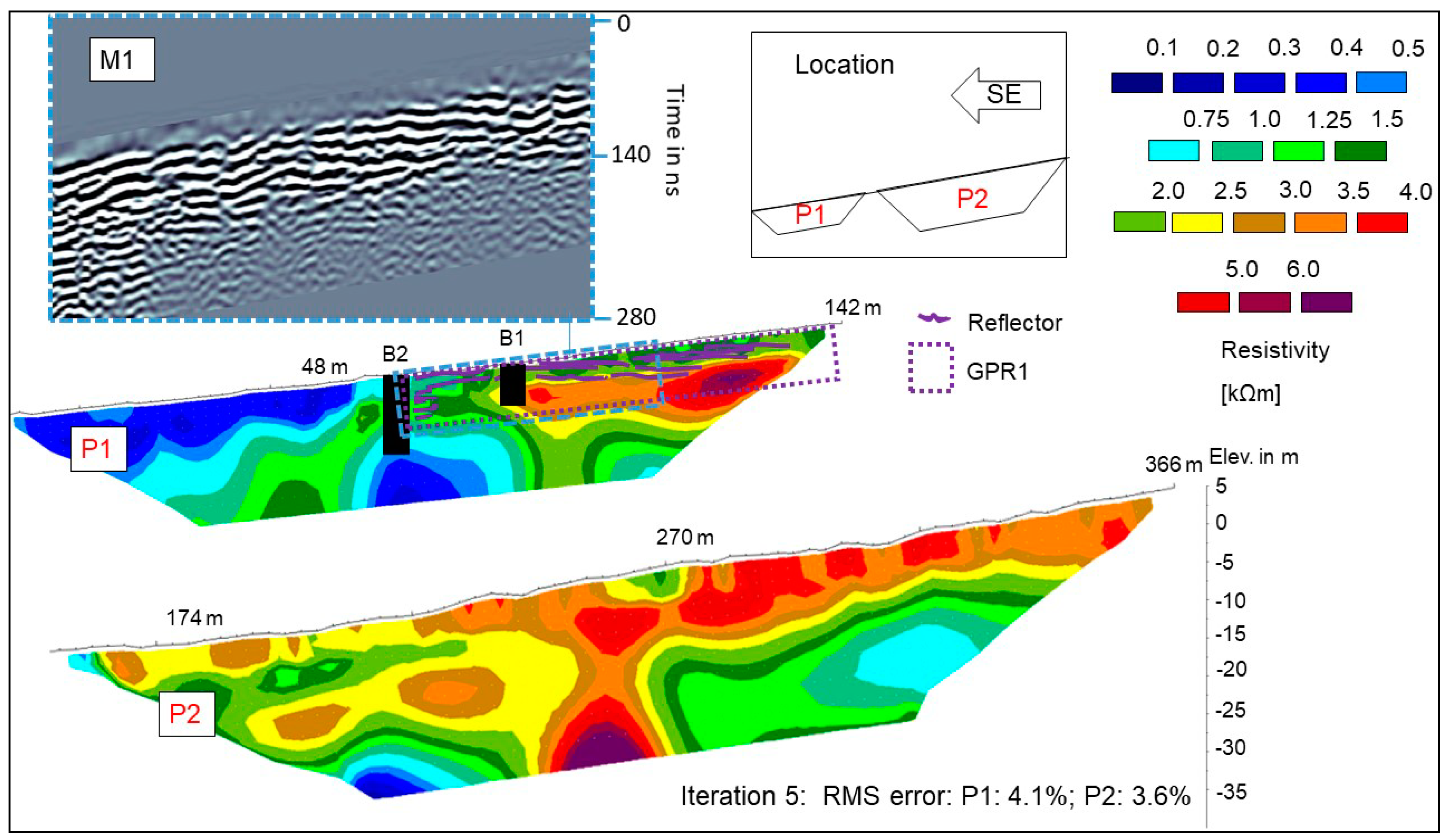
The primary methods employed to prospect the peatlands and their catchment area were ERT, GPR and rammed Boreholes (B). For the measurements of the ERT, Syscal/Pro and Syscal Junior Switch 72 (Iris Instruments, Orléans, France) were used. ERT makes use of the fact that every material has a different conductivity. The conductivity is also coupled to several different properties, such as water saturation, temperature, the chemistry of the pore water, etc. The software package, Res2dinv (Geotomo Software, Penang, Malaysia), was used to invert the data. To retain a high quality of the ERT data, all quadripoles with a deviation of 5% or higher between the single measurements were deleted. The total resolution index was calculated, and parts with a lower index than five have not been interpreted.
In all profiles, the fifth iteration of the standard least square inversion (L2-norm) is shown, since these results showed a better fitting to the lithological conditions, compared to the robust inversion (L1-norm) scheme, which was also applied. After the fifth iteration, no significant change in the RMS error had occurred. The scale for the resistivity values in the tomograms was designed to display all interpreted areas in one color scale. Wenner-Schlumberger arrays, with 2-m and 3-m spacing consisting of 936 quadripoles and 72 electrodes, were applied for the characterization of the subsurface lithology. To create longer profiles but retain a high resolution in the drained part of the “Thranenbruch” site and at “Gebranntes Bruch”, ERT using the roll-along method was executed. For this approach, several measurements were combined. Thirty-six of the 72 electrodes of the 936 quadripole-sequences were removed and rolled along to obtain a longer distance. The profiles and electrodes were located using a differential GPS system (Leica, Wetzlar, Germany) with Real Time Kinematic (RTK). We used a rover (GS14) and base (GS10) system. In areas with poor satellite reception, the position of the electrodes was obtained manually and was subsequently evaluated using a DEM.
The fixed electrodes at the monitoring site were measured monthly. The time-lapse data were inverted independently, and the percentage difference was calculated. Monitoring1 was used, with 1-m spacing and 36 electrodes, while Monitoring2 had 2-m spacing, using 72 electrodes. Both monitoring sites were measured using the Wenner-Schlumberger configuration.
The GPR measurements were meant to show the boundaries of different layers and the changes of them in different parts of the sections to support the ERT measurements. Along the ERT profiles, GPR surveys (Sensors & Software, Mississauga, ON, Canada) were performed using 100MHz antennas. In the catchment area of “Thranenbruch”, only a small section of the profiles could be measured in such a way. The data were filtered using a bandpass filter (Fc1:40, Fp1:80; Fp2:120, Fc2:160), and the topography was migrated via GPS data or by LIDAR data, depending on the satellite reception. The displayed data were gained by SEC2Gain, with an attenuation of six, a starting value of four, with a maximum value of 500. Additionally, a background subtraction was carried out. All operations have been performed using the software, Ekko_Project (Sensors & Software, Mississauga, ON, Canada). The main reflectors of the GPR surveys are marked within the ERT section, and the most important changes and anomalies are shown in magnified parts, including the raw GPR data.
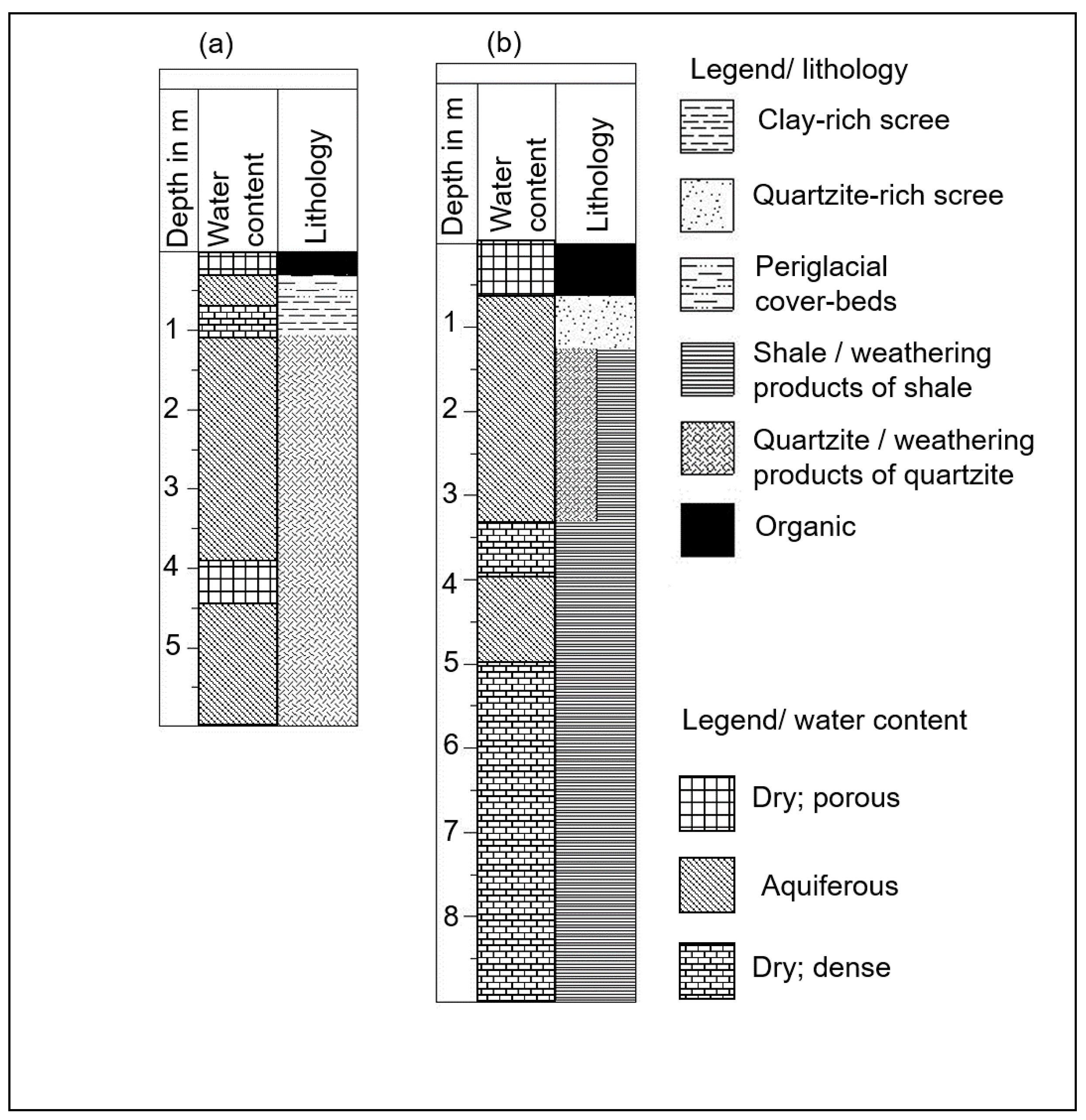
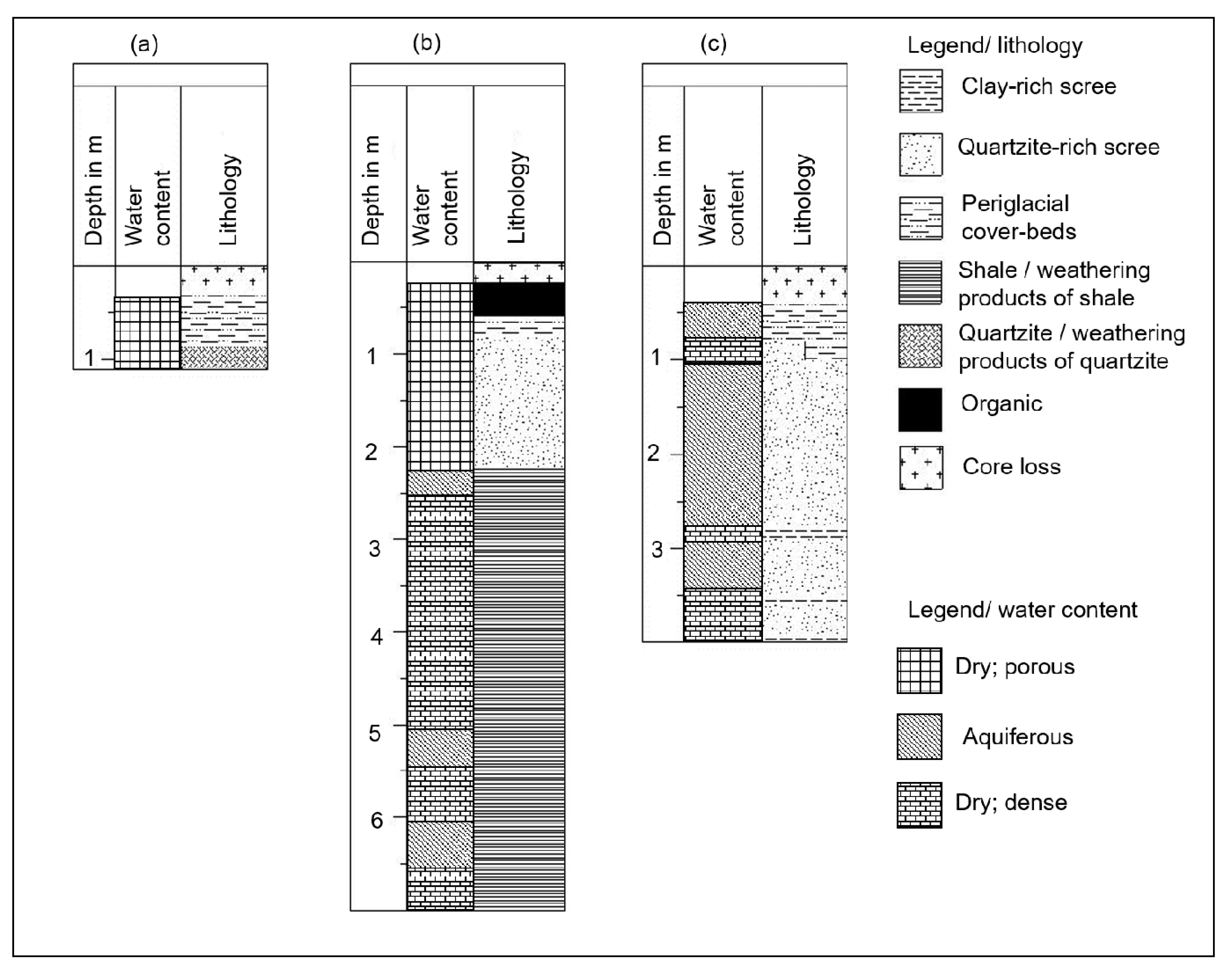
To support the interpretation of the geophysical data, at least two boreholes at each part of the study sites were performed to obtain direct data on the structure and layering of the subsurface. The borehole location was selected to cover typical slope sections and also at the position of anomalies, found through the interpretation of the geophysical data. The boreholes were rammed using a Wacker Neuson BH65 (Wacker Neuson, Munich, Germany) demolition hammer. The obtained window samples of a diameter of 30–80mm were described after WRB in the field [28]. The hydrological and sedimentological investigations of the described window samples are generalized.
Within the “Thranenbruch”, data were collected along two transects. The first transect was located within the catchment area of the peatland and extended into the wet parts. The second location was within the drained part of the former peatland. The collected data in the catchment area of “Thranenbruch” extended from a beech forest (P2) into the wet parts of the peatland (P1). In contrast to the other locations, it was neither possible to create a roll-along ERT profile nor to execute longer GPR profiles than the one shown due to dense vegetation and considerable topography.
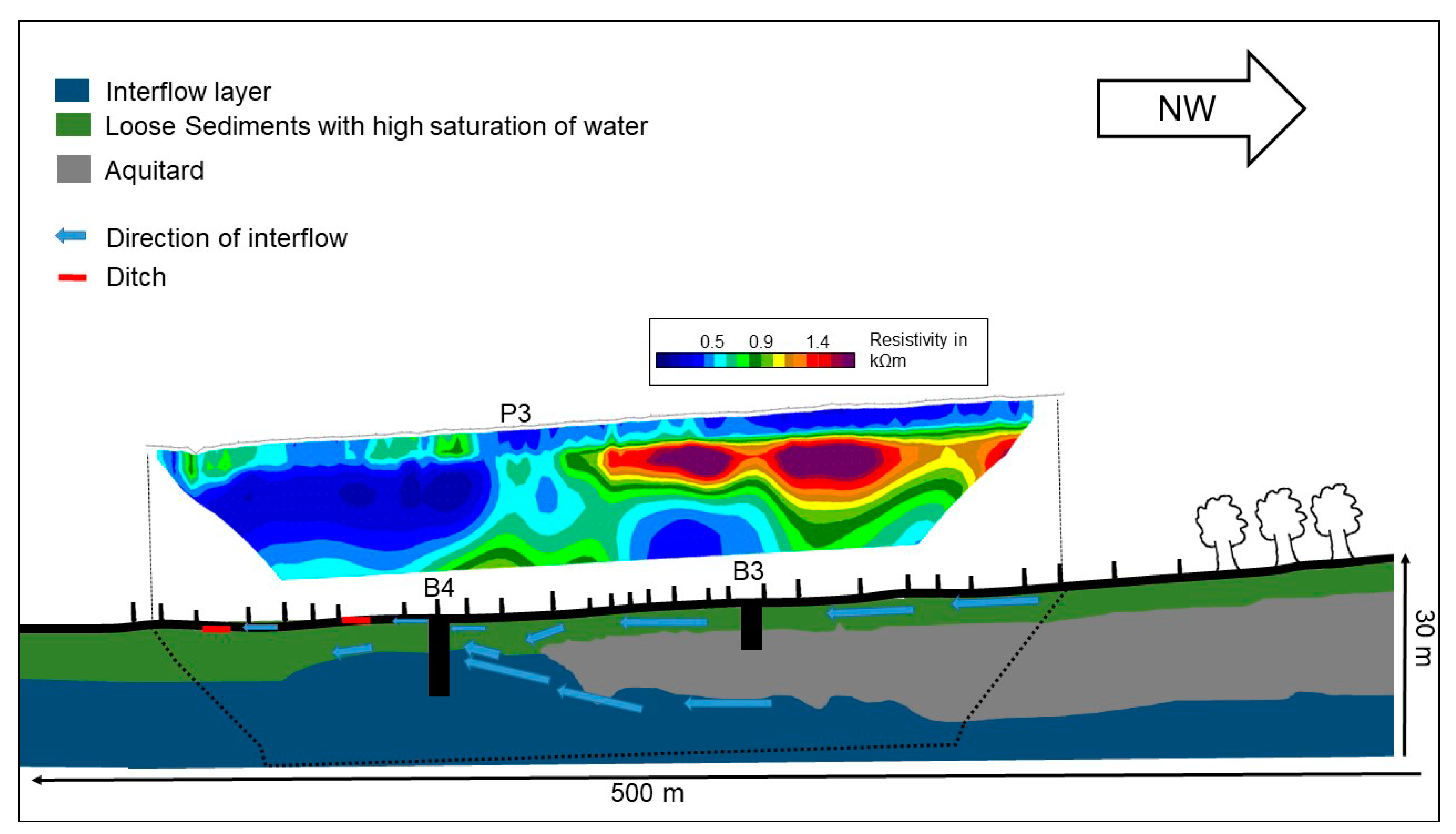
At the “Gebranntes Bruch” site, a similar methodological setup to the drained part of “Thranenbruch” was undertaken, boreholes were drilled, and an ERT transect through the catchment area and the wet parts of the peatland, combined with a GPR survey of the same length, were performed.

3. Results and Interpretation

3.1. Case Study Site “Thranenbruch”

3.1.1. Catchment Area of “Thranenbruch”

ERT

In the uphill part of profile P1 (Figure 4), three layers are visible in the ERT. The uppermost and the bottom layer have a relatively low resistance (around 1 kΩm), while the intermediate layer shows higher resistivity values (around 3 kΩm). At around meter 64 of the ERT, the bottom layer drops out at the top, with decreasing resistivity values. Underneath this layer, the resistivity values increase again (around 1 kΩm).
In the uphill part of P2, two layers are visible. A higher resistive layer (3–4 kΩm) is shown at the top, and a relatively low resistive layer at the bottom (around 1 kΩm). Underneath a track (located at meter 270 in the ERT section), an anomaly, with higher resistivity values (>5 kΩm), is present. Downhill of this anomaly, up to four alternating high and low resistive layers are visible. While the resistivity values in the low resistive area are below 1 kΩm, in the higher resistive areas, between 2 and 3 kΩm are present.

GPR

Profile GPR1 (Figure 4) started at the end of P1 and terminated inside the peatland, around the middle of the ERT profile P1. In the uphill part of GPR1, a clear horizontal layering is visible. This layering changes from a clear horizontal one to a diffuse one further downhill (Figure 4:M1). Additionally, different layers, located below the horizontal layering, drop out closer to the surface, towards the downhill part.

Boreholes

B1 (Figure 5a) depicts periglacial cover-beds on the top of quartzite regolith. The quartzite regolith at this location is impossible to penetrate using the drilling equipment. Both layers are almost dry.
B2 (Figure 5b) shows wet and dry layers below a depth of 0.8 m. These layers are partly made of clay-rich scree, partly of weathered quartzite-rich scree. While the quartzite-rich scree acts mostly as a water-bearing layer (aquiferous), the clay-rich scree is mostly dense and can be classified as aquitard. Some layers are a mixture of both materials.

Geoelectrical Monitoring

Monitoring1 shows three layers of different resistivity values (Figure 6a–d). Within the uppermost parts of the profile, two layers are visible. The northwestern part of the profile shows resistivity values between 0.5 and 0.8 kΩm, while the resistivity of the uppermost southeastern part fluctuates between 0.25 and 0.5 kΩm. Both layers end up at a depth of around 2 m. The bottom layer, underneath these two layers, is heterogeneous, with relatively low resistivity values, between 0.1 and 0.4 kΩm. Figure 6f shows the 10-day average temperature before the measurement and the cumulated precipitation for these days.
Figure 6e displays the results of a time-lapse inversion of July 2017 and February 2018 for the data obtained at Monitoring1. The percentage difference of the resistivity values of both measurements is calculated. The resistivity values of the uppermost layers fluctuate during the different measurement times (up to 25%), while the resistivity values within the bottom layer are more or less stable (changes between −5% and 10%).

3.1.2. Drained Part of “Thranenbruch”

ERT

P3 (Figure 7) shows three parts with different distributions of resistivity values within the area of investigation. The uppermost layer has low resistivity values. Until meter 110 in the ERT section, there is a high resistive area (around 1.5 kΩm) below, at a depth of about 2 m. This high resistive layer is underlain by a layer with lower resistivity values (around 0.5 kΩm). In the middle part, starting at meter 110 in the ERT section, a layer with higher resistivity values drops out. However, a layer with lower resistivity values (around 0.5 kΩm) on the top of a layer, with higher resistivity values, is present. In the downhill part of P3, the uppermost layer shows increasing resistivity values, while the resistivity value of the bottom layer is around 0.1 kΩm. Underneath both layers, the resistivity value increases.

GPR

The data of GPR2 confirm the subdivision of ERT P3 into three parts. Inside the uphill part of GPR2, a clear horizontal layering is visible. In the middle part, different layers, located underneath the horizontal layers, drop out, and inside the downhill part, diffuse reflectors on top of a stronger reflector have been detected (Figure 7:M2).

Boreholes

B3 (Figure 8a) shows wet periglacial cover-beds in the uppermost layers, overlying weathering products of quartzite. The water table inside the borehole was about 20 cm below the ground surface. The borehole was drilled during a hot summer period, before the ditches were refilled. B4 (Figure 8b) shows a fossil peat layer at the top, suggesting the previous existence of a peatland. Beneath the peat layer, there is a mixture of clay-rich scree and quartzite-rich scree until a depth of 5 m. Below this depth, only gravels made of claystone and clay can be found. The water table inside the hole was about 80 cm below the ground surface.

Geoelectrical Monitoring

Monitoring2 (Figure 9) and Monitoring1 were measured on the same dates. Monitoring2 is part of P3 and ends at the same place. Therefore, the description of the resistivity distribution is analogous to the last 142 m of P3. The resistivity values of Figure 9a–d varied only slightly during the different dates of measurement, especially below a depth of 2 m. Figure 9e displays the results of the time-lapse inversion of the data, from July 2017 and February 2018, for Monitoring2. The resistivity values within the uppermost layer fluctuate by up to 60%. Below the first depth of 2 m, the resistivity values stay stable or even become contrasting to the top (–15–0%), notwithstanding the different meteorological conditions (Figure 6f).

3.2. “Gebranntes Bruch”

3.2.1. ERT

In the northwestern part of the ERT section (Figure 10), high resistivity values (>5 kΩm) are recorded until a depth of 10 m. Below this layer, the resistivity values decrease (2 kΩm). At meter 64 in the ERT section, the profile intersects with a forest track. In this part of the profile, there is a layer with lower resistivity values (around 1 kΩm) near the surface and another one at the bottom of the profile, with a higher resistive area (around 5 kΩm) nested in between. At meter 160 in the ERT section, it seems that the bottom layer with lower resistivity values dropped out at the surface, which was caused by a high resistive anomaly, starting at the bottom of the profile. Further downhill, at a depth of 1–2 m, there are again some layers with higher resistivity values. On top and below these layers, there are areas with lower resistivity values (around 1 kΩm). Starting at the anomaly at meter 230 in the ERT section, a higher resistive layer (>5 kΩm) occurs at the bottom of the profile to a depth of 15 m. At the end of the ERT section, slightly higher resistivity values (around 2 kΩm), until a depth of 2 m, are visible underneath the low resistive layer.

3.2.2. GPR

Uphill of the track, M3 shows several layers dropping out at the surface (Figure 10:M3). Below these layers, some surface parallel layers are visible. The dropping out of the layers at meter 160 in the ERT section is confirmed by M4 (Figure 10:M4). M5 shows several diffuse layers on top of a downwelling layer (Figure 10:M5).

3.2.3. Boreholes

In B5 (Figure 11a), periglacial cover-beds, underlain by quartzite regolith, are documented. The whole borehole is dry. The first meters of B6 (Figure 11b), located at meter 102 in the ERT section, were almost dry. A small fossil peat layer indicates that there were wetter conditions in the past. Below the peat, periglacial cover-beds occur on top of quartzite-rich scree. Below a depth of 2.30 m, the quartzite-rich scree drops out, and clay-rich layers are located. These clay-rich layers are partly heavily weathered and can be classified as aquitard, whereas other parts remain less weathered and are aquiferous. Until a depth of 7 m, reduction and oxidation elements indicate the spatio-temporal influence of water. Through the findings of the drilling at B7 (Figure 11c), these different layers are confirmed. In contrast to B6, more different layers occur, and quartzite-rich scree and clay-rich scree alternate frequently. The different layers can either be classified as aquitard or permeable.

3.3. Conceptual Models of the Subsurface Lithological and Hydrological Conditions

The conceptual models are based on the combination of ERT and GPR data, with the sediment description obtained from the boreholes. Furthermore, the models are confirmed by several different parallel and diagonal ERT surveys, with spacings between 1 and 5 m and lengths between 35 and over 450 m (not shown). Additionally, GPR surveys were conducted using 50 MHz antennas, and findings from seismic refraction surveys (not shown) support the deduced conceptual models.

3.3.1. “Thranenbruch”

The ditches in this area do not drain all the moisture from the peatland. Therefore, it is still wet enough to retain peat layers in the wetter parts of the “Thranenbruch”.

Catchment Area of “Thranenbruch”

Model1 (Figure 12) shows the wet part, including the catchment area of the “Thranenbruch”. In the catchment area, quartzite is the dominating lithology (B1). This rock is jointed and fractured, allowing water to pass through until it reaches impermeable layers [4]. Periglacial cover-beds have been deposited on top of the quartzite. These layers have a low clay content and enable infiltrating water to percolate. Below the quartzite, the structural conditions suggest the presence of Hunsrueck shale. The forest track seems to have a strong impact on the subsurface water flow distribution. It appears that water collected on top of the shale laterally flows downhill until the track intersects (P2). It is possible that the track dams the water by compressing the regolith. Downhill of the track, the lithological and hydrological conditions are more diffuse. There are several different layers. The water constituting the interflow is able to avoid the proposed damming area of the track and passes this anomaly at a greater depth under pressure. Hence, this bottom layer shows the lowest resistivity values. The other layers partly consist of quartzite and partly of shale. In the last hundred meters of the catchment area, the vegetation changes from beeches to spruces, and the lithology becomes more structured. The dry periglacial cover-beds and the high resistive quartzite warrant the assumption that the water feeding the peatland still flows underneath the quartzite. Once the bottom layer drops out to the surface (P1, GPR1), vegetation changes from a spruce-dominated forest to a peatland dominated in particular, by Molinia caerulea. Here, the water of the catchment area reaches the surface.
GPR1 shows a high number of different layers at the top edge of the peatland. B2 shows that some of those layers are aquiferous, some act as aquitard, some have a high clay content, and some include quartzite regolith. Hence, underneath the peatland, scree and regolith of different bedrock types occur. Within the peatland, the resistivity values all over the profile are quite low; therefore, no further differentiation of the subsurface substrate could be conducted yet. Even though P1 and P2, as well as GPR1 and the invasive data, display a temporal point measurement, Monitoring1 indicates a more or less stable hydrological system underneath the uppermost meters, notwithstanding changing meteorological conditions.

Drained Part of “Thranenbruch”

At first glance, the subsurface of the drained part of “Thranenbruch” (Figure 13) seems to be comparable to the subsurface of the wet part and its catchment area, at least if only the ERT data are considered (Figure 4 and Figure 7). Uphill, there are periglacial cover-beds on top of quartzite (B3) in a surface parallel layering (GPR2). In the middle part of the model, near the bottom, layers with lower resistivity values, possibly shale or water-bearing material, drop out to the surface. Further downhill, this layer is still at the surface, but it is drained by ditches that pass through this area.
In contrast to these results, in both boreholes (B3 and B4), the water table was close to the surface. Therefore, a high amount of water does not pass through the lower resistive bottom part, although it at least flows through the periglacial cover-beds on top of the quartzite. The hydrological system of the drained part of “Thranenbruch” is driven by the interflow through the bedrock and also by water flowing inside the periglacial cover-beds.
Within the whole “Thranenbruch” area, the hydrological system seems to be more complex than has previously been assumed. Even though ditches run through the drained part as well as the less-affected part of the peatland, they experience different degradation stages. Removing the spruce and re-filling the ditches could help to re-nature the ecosystem. Without deeper knowledge of the hydrological conditions, the changes may also have no effect. By comparison, in B1 and B3, we see that the drained part seems to have a better hydrological coupling than the wet part, notwithstanding the different natural statuses. The results of Monitoring2 confirm the temporal point measurements of Model2 below a depth of 2 m during different meteorological conditions. The fluctuating resistivity values of the uppermost layer indicate a variable moisture content within these layers. Especially, the uppermost layer is less stable under varying meteorological conditions, and the water table shown in B3 and B4 is probably more variable than that shown in Model2.

3.3.2. “Gebranntes Bruch”

Model3 (Figure 14) indicates that the situation in “Gebranntes Bruch” is partly comparable to the one in “Thranenbruch”. According to the geological map (Figure 1e), clay shale layers are embedded within quartzite bedrock. While these layers are well segmented in the first section of the peatland (B6, GPR3), they are more heterogeneous downslope (B7). Inside these layers, there are parts acting as aquitard and others as water-bearing. Wherever these aquifers drop out at the surface, water feeds the peatland (M4). Due to the high amount of water, it is necessary that the aquiferous layers have a bigger catchment area and obtain their moisture from the parts below the jointed quartzite uphill. Hence, this peatland is fed more by interflow than precipitation. As documented in B7 and M5, there must be areas within the bedrock which act as sediment traps and are filled with scree. While the GPR-data indicate this differentiation (M6), the ERT data do not support this assumption.

4. Discussion and Conclusions

The presented findings are based on single measurements; nevertheless, the integration of the geoelectrical monitoring data, collected at different times of the year, allowed representative conceptual models, related to different meteorological situations, to be deduced. While the water content of the uppermost layers changes with weather conditions, the bottom layer seems to be more stable and changes to a lesser extent. The ecological classification, as a transition bog [4], can be confirmed hydrogenetically as a slope bog. The direct precipitation influences the hydrology of the peatland as well as the interflow in the subsurface. Especially, the monitoring data in combination with the precipitation and temperature data indicate that there are several forces that drive the hydrology and hydrogeology of the peatlands.
The results of our study agree partly with the statements from other scholars [5], who suggest that the water passes the permeable quartzite and flows on the aquitard shale downslope. Where the shale drops out close to the scree, the interflow on top of this aquitard layer flows to the surface and creates a spring, feeding the peatlands. Especially, the clay-rich regolith and scree, as well as the cover-beds, reduced the re-infiltrating into the subsurface and stagnant conditions on top of these layers. It should be noted that shale is not the sole supplier of aquitard material. Another scholar showed different areas in which slope bogs are common, without the dropping out of quartzite on top of shale [4], while yet another indicated that clay-rich layers inside the quartzite and the partly impermeable quartzite itself supply those layers [25]. Our results support these assumptions.
Even though clay-rich periglacial cover-beds are documented in the boreholes, the results indicate that high water contents, with the accumulation of peat, are more common in clay-rich shale regolith or scree than above periglacial cover-beds. This stands in contrast to the results of one scholar [29] for the Eastern Hunsrueck, where the clay-rich periglacial cover-beds caused stagnant conditions and impeded the infiltrating of water.
The results of the ERT and the GPR indicate an anticlinal folding of the horsts [24,25] in “Thranenbruch”, while there is no hint in the data of “Gebranntes Bruch” of a folding. Especially, the angle between the top of different layers and the surface are in support of this. However, the presented results are not meant to display the folding.
Clay-rich layers show a high electrical conductivity, similar to layers with high water saturation or peat content [30,31]. Therefore, it is not always easy to determine whether the detected areas, with lower resistivity values, are saturated with water or have a high clay content, or both. One scholar already described the same problem in peatlands in Egypt [32]. As a consequence, it seems to be advisable to try to collect more direct data through drilling at other sites. Other scholars have demonstrated that the resistivity of wet peat can be in the range of 150–370 Ωm [6,11]. In other areas of investigation, even resistivity values below 50 Ωm are documented [12,15]. In this study, the range is even higher than 370 Ωm (up to 800 Ωm). The reason for the slightly higher resistivity of the peat in our study sites could be the small-sized peat bodies in parts of the “Thranenbruch”, which only had a peat thickness of between 0.4 and 1.10 m, and the influence of anthropogenic drainage still being strong, the peat could partly not even be displayed within the ERT data of Monitoring1. Nevertheless, scholars have reported a high variability of conductivity even in a single peatland due to a difference in pH values, the mineral input of the precipitation, and mineralization within the peatland [33]. Additionally, the inflow of the water feeding the peatland can have various resistivity values, which change a lot in time and space [15]. The more or less stable resistivity values of the monitoring data, underneath the uppermost two meters, indicate that this seems not to be the main reason for the high values. The variability of resistivity is even higher if different peatlands are compared [34]. Caused by the small sizes of the peat in our area of investigation, parts of them can only be displayed within Monitoring1, with 1-m spacing. However, the range of the resistivity of the other lithology elements is quite high, but still within a typical range [35,36]. Compared to other studies [14,37], it was not possible to point out distinct layers within the peat body with the GPR antennas used; however, the GPR results could be used to support the interpretation of the ERT data.
Nonetheless, one scholar indicated a higher influence of the site and soil characteristics on the interflow runoff than the forest type [38], however the influence from vegetation on interflow resistivity distribution is still high [19]. Especially, the spruce with a high water consumption and interception [39] has a huge impact on water distribution and needs further investigation.
Based on our findings from the field measurements, the hydrological conditions of “Gebranntes Bruch” seem less complex than those of “Thranenbruch”. Below the forest track (e.g., Figure 1), shale layers are documented within quartzite. Wherever the shale drops out at the surface, the dammed water on top feeds the peatland.
The conceptual models are based on several different data and the interpretation of these data (i.e., additional ERT measurements, with between 1-m and 5-m spacing, GPR-profiles, with 50 MHz antennas, and seismic refraction). Due to the high number of datasets, only the most representative data are shown. Nevertheless, the deepest parts of the models have an especially thin database.
The study demonstrates the value of subsurface investigations to obtain insights into the catchment areas of peatlands. While the need of a catchment area for this type of bog is already known, our work shows the high number of different interflow layers in a complex hydrogeological system. The non-invasive ERT is not only a promising method when applied within bogs and peatlands, but it also finds suitable application within their catchment areas. ERT assists a characterization of the subsurface lithology and hydrogeological conditions, because it makes the different paths of water visible. However, it should be supported by other methods, such as GPR, and the findings should be confirmed by direct methods, such as borehole drilling. At the selected case study sites, small differences in subsurface properties can have a huge impact on the subsurface hydrogeology and the water paths. The results and interpretation presented herein allow us to delineate the different and complex subsurface water pathways within the catchment area of slope bogs. The knowledge of the complex hydrology of the catchment areas and the different aquifers feeding the slope bogs enables a better protection and renaturation of these rare ecosystems. More research, with a higher spatial coverage, would be helpful for improving the different protection efforts.

Author Contributions

Conceptualization, J.T. and C.K.; Methodology, J.T. and C.K.; Software, J.T. and C.K.; Validation, J.T. and C.K.; Writing—Original Draft Preparation, J.T. and C.K.; Visualization, J.T.; Supervision, C.K.; Project Administration, C.K.; Funding Acquisition, C.K.

Funding

The research was funded by the Federal Ministry of Food and Agriculture [Bundeslandwirtschaftsministerium, BMEL] and Federal Ministry for the Environment, Nature Conservation and Nuclear Safety [Bundesumweltministerium, BMU] in the framework of the Waldklimafonds [28WA4096]. This publication was financially supported by the German Research Foundation [DFG] and the University of Wuerzburg in the funding program, Open Access Publishing.

Acknowledgments

The authors would like to thank the two anonymous reviewers for their useful comments and suggestions.

Conflicts of Interest

The authors declare no conflict of interest.

References

  1. Reichert, H. Die Quellmoore (Brücher) des südwestlichen Hunsrück. Beitr. Landespfl. Rheinl. Pfalz 1975, 3, 101–166. [Google Scholar]
  2. Hofmann, D. Die Brücher des Hochwaldes. Mitt. Forsteinrichtungsamt Kobl. 1957, 6, 1–30. [Google Scholar]
  3. König, D.; Egidi, H.; Herrmann, M.; Schultheiß, J.; Tempel, M.; Zemke, J. Der Nationalpark Hunsrück-Hochwald—Naturräumliche Austattung und anthropogene Überprägung. Koblenzer Geographisches Kolloquium 2015, 36–37, 6–42. [Google Scholar]
  4. Scholtes, M. Die Brücher—Mittelgebirgsmoore im Hunsrück dargestellt am Beispiel des NSG “Hangbrücher bei Morbach”. Telma 2002, 22, 63–106. [Google Scholar]
  5. Lehmann, L. Bodenkarte 1:5000, Erläuterungen zur Bodenkarte 1:5000, NsG Hangbrücher bei Morbach und geplantes NSG Hangbrücher bei Hochscheid; Expert Report for Landesamt für Umwelschutz und Gewerbeaufsicht: Mainz, Germany, 1986. [Google Scholar]
  6. Comas, X.; Terry, N.; Slater, L.; Warren, M.; Kolka, R.; Kristiyono, A.; Sudiana, N.; Nurjaman, D.; Darusman, T. Imaging tropical peatlands in Indonesia using ground-penetrating radar (GPR) and electrical resistivity imaging (ERI): Implications for carbon stock estimates and peat soil characterization. Biogeoscience 2015, 12, 2995–3007. [Google Scholar] [CrossRef]
  7. Sonnentag, O.; Chen, J.M.; Roulet, N.T.; Ju, W.; Govind, A. Spatially explicit simulation of peatland hydrology and carbon dioxide exchange: Influence of mesoscale topography. J. Geophys. Res. 2008, 113. [Google Scholar] [CrossRef]
  8. Knox, S.H.; Sturtevant, C.; Matthes, J.H.; Koteen, L.; Verfallie, J.; Baldocchi, D. Agricultural peatland Restoration: Effects of land-use change on greenhouse gas (CO2 and CH4) fluxes in the Sacramento-San Joaquin Delta. Glob. Chang. Biol. 2015, 21, 750–765. [Google Scholar] [CrossRef] [PubMed]
  9. Comas, X.; Slater, L.; Reeve, A.S. Pool patterning in a northern peatland: Geophysical evidence for the role of postglacial landforms. J. Hydrol. 2011, 399, 173–184. [Google Scholar] [CrossRef]
  10. Slater, L.; Comas, C.; Ntarlagiannis, D.; Moulik, M.R. Resistivity-based monitoring of biogenic gases in peat soils. Water Resour. Res. 2007, 43, W10430. [Google Scholar] [CrossRef]
  11. Sass, O.; Friedmann, A.; Haselwanter, G.; Wetztel, K.-F. Investigating thickness and internal structure of alpine mires using conventional and geophysical techniques. Catena 2010, 80, 195–203. [Google Scholar] [CrossRef]
  12. Bechtel, T.D.; Goldschneider, N. Geoelectrical Fingerprinting of Two Contrasting Ecohydrological Peatland Types in the Alps. Wetlands 2017, 37, 875–884. [Google Scholar] [CrossRef]
  13. Götz, J.; Salcher, B.; Starnberger, R.; Krisai, R. Geophysical, topographic and stratigraphic analyses of perialpine kettles and implications for postglacial mire formation. Geogr. Ann. Ser. A Phys. Geogr. 2018, 100, 254–271. [Google Scholar] [CrossRef]
  14. Walter, J.; Hamann, G.; Lück, E.; Klingenfuss, C.; Zeitz, J. Stratigraphy and soil of fens: Geophysical case studies from northeastern Germany. Catena 2016, 142, 112–125. [Google Scholar] [CrossRef]
  15. Kowalczyk, S.; Żukowska, K.A.; Mendecki, M.J.; Łukasiak, D. Application of electrical resistivity imaging (ERI) for the assessment of peat properties: A case study of the Całowanie Fen, Central Poland. Acta Geophys. 2017, 65, 223–235. [Google Scholar] [CrossRef]
  16. Kneisel, C.; Emmert, A.; Polich, P.; Zollinger, B.; Egli, M. Soil geomorphology and frozen ground conditions at a subalpine talus slope having permafrost in the eastern Swiss Alps. Catena 2015, 133, 107–118. [Google Scholar] [CrossRef]
  17. Bermejo, L.; Ortega, A.I.; Guérin, R.; Benito-Calvo, A.; Pérez-Gonzáles, A.; Páres, J.M.; Aracil, E.; De Castro, J.M.B.; Carbonell, E. 2D and 3D ERT imaging for identifying karst morphologies in the archaeological sites of Gran Dolina and Galería Complex (Sierra de Atapuerca, Burgos, Spain). Quart. In. 2017, 433, 393–401. [Google Scholar] [CrossRef]
  18. Palis, E.; Lebourg, T.; Vidal, M.; Levy, C.; Tric, E. Hernandez, M. Multiyear time-lapse ERT to study short- and long-term landslide hydrological dynamics. Landslides 2017, 14, 1333–1343. [Google Scholar] [CrossRef]
  19. Ma, Y.; van Dam, R.L.; Jayawickreme, D.H. Soil moisture variability in a temperate deciduous forest: Insights from electrical resistivity and throughfall data. Environ. Earth Sci. 2014, 72, 1367–1381. [Google Scholar] [CrossRef]
  20. Brunet, P.; Clément, R.; Bouvier, C. Monitoring soil water content and deficit using Electrical Resistivity Tomography (ERT)—A case study in the Cevennes area, France. J. Hydrol. 2010, 380, 146–153. [Google Scholar] [CrossRef]
  21. Uhlemann, S.S.; Sorensen, J.P.R.; House, A.R.; Wilkinson, P.B.; Roberts, C.; Goody, D.C.; Binley, A.M.; Chambers, J.E. Integrated time-lapse geoelectrical imaging of wetland hydrological processes. Water Recour. Res. 2016, 52, 1607–1625. [Google Scholar] [CrossRef]
  22. Schilling, K.E.; Jacobson, P.J.; Streeter, M.T.; Jones, C.S. Groundwater Hydrology and Quality in Drained Wetlands of the Des Moines Lobe in Iowa. Wetlands 2018, 38, 247–259. [Google Scholar] [CrossRef]
  23. Volik, O.; Petrone, R.M.; Wells, C.M.; Price, J.S. Impact of Salinity, Hydrology and Vegetation on Long-Term Carbon Accumulation in a Saline Boreal Peatland and its Implication for Peatland Reclamation in the Athabasca Oil Sands Region. Wetlands 2018, 38, 373–382. [Google Scholar] [CrossRef]
  24. Wildberger, J. Zur tektonischen Entwicklung des südwestlichen Hunsrücks (SW-Deutschland). Mitt. Pollichia 1992, 79, 5–119. [Google Scholar]
  25. Martin, E. Der Tausnusquarzit im nordöstlichen Soonwald—Analyse eines Kluftwasserspeichers. Mainz. Geowiss. Mitt. 1984, 13, 299–355. [Google Scholar]
  26. Zöller, L. Über Handschuttbildung, Plateaulehme und junge Erosion im “Hochwald”. Catena 1980, 7, 153–167. [Google Scholar] [CrossRef]
  27. Grebe, H.; Leppla, A. Erläuterungen zur Geologischen Specialkarte von Preussen und den Thüringischen Statten, Lieferung 63, Gradabteilung 80, No. 17; Simon Schropp´schen Hof-Landkartenhandlung: Berlin, Germany, 1898. [Google Scholar]
  28. FAO (Food and Agriculture Organization of United Nation). World reference base for soil resources 2014 updated 2015. World Soil Resour. Rep. 2015, 106, 153–154. [Google Scholar]
  29. Felix-Henningsen, P.; Spies, E.-D.; Zakosek, H. Genese und Stratigraphie periglazialer Deckschichten auf der Hochfläche des Ost-Hunsrücks (Rheinisches Schiefergebirge). E&G Quat. Sci. J. 1991, 41, 56–69. [Google Scholar] [CrossRef]
  30. Fukue, M.; Minato, T.; Horibe, H.; Taya, N. The micro-structures of clay given by resistivity measurements. Eng. Geol. 1999, 54, 43–53. [Google Scholar] [CrossRef]
  31. Besson, A.; Cousin, I.; Samouëlian, A.; Boizard, H.; Richard, G. Structural heterogeneity of the soil tilled layer as characterized by 2D electrical resistivity surveying. Soil Tillage Res. 2004, 79, 239–249. [Google Scholar] [CrossRef]
  32. El-Ghadi, A.; El-Qady, G.; Metwaly, M.; Awad, S. Mapping peat layer using surface geoelectrical methods at Mansoura Environs, Nile Delta, Egypt. Mansoura J. Geol. Geophys. 2007, 34, 59–77. [Google Scholar]
  33. Maier, R.; Punz, W.; Domschitz, E.; Nagl, A.; Neumann, G.; Plefka, E.; Teuschl, G.; Korner, I.; Hammer, O.; Hudler, P.; et al. Beiträge zur Ökophysiologie von Betula nana auf einem Hochmoor in Lungau (Salzburg). Verh. Zool.-Bot. Ges. Österr. 1985, 123, 151–174. [Google Scholar]
  34. Walter, J.; Lück, E.; Bauriegel, A.; Richter, C.; Zeitz, J. Multi-scale analysis of electrical conductivity of peatlands for the assessment of peat properties. Eur. J. Soil Sci. 2015, 66, 639–650. [Google Scholar] [CrossRef]
  35. Palacky, G.J. Clay mapping using electromagnetic methods. First Break 1987, 5, 295–3063. [Google Scholar] [CrossRef]
  36. Reynolds, J.M. An Introduction to Applied and Environmental Geophysics, 2nd ed.; Wiley-Blackwell: Chichester, UK, 2011. [Google Scholar]
  37. Pereira, D.; Dias, E.; Ponte, M. Investigating the internal structure of four Azorean Sphagnum bogs using ground-penetrating radar. Mires Peat 2017, 19, 1–9. [Google Scholar] [CrossRef]
  38. Hümann, M.; Schüler, G.; Müller, C.; Schneider, R.; Johst, M.; Caspari, T. Identification of runoff processes—The impact of different forest types and soil properties on runoff formation and floods. J. Hydrol. 2011, 409, 637–649. [Google Scholar] [CrossRef]
  39. Lyr, H.; Fiedler, H.-J.; Tranquillini, W. Physiologie und Ökologie der Gehölze; Gustav Fischer Verlag: Jena, Germany, 1992. [Google Scholar]
Figure 1. Location of the study sites: (a) overview (Basemap: Esri-basemap-Topographic-10 October 2018), (b) profile of “Thranenbruch” (Basemap: TK 25, 6208, Morscheid-Riedenburg), (c) profile of “Gebranntes Bruch” (Basemap: TK 25, 6109, Hottenbach), (d) geological map of “Thranenbruch” (Basemap: GK 25, 6208, Morscheid), (e) geological map of “Gebranntes Bruch” (Basemap: GK 25, 6109, Hottenbach), (f) photograph of “Thranenbruch”, (g) photograph of “Gebranntes Bruch”.
Geosciences 09 00118 g001
Figure 2. Climate graph for Hüttgeswasen.
Geosciences 09 00118 g002
Figure 3. Aerial photograph of “Thranenbruch” taken from a drone (1 June 2008).
Geosciences 09 00118 g003
Figure 4. Geophysical surveys in the catchment area of “Thranenbruch”.
Geosciences 09 00118 g004
Figure 5. Boreholes: catchment area of “Thranenbruch”: (a) B1, (b) B2.
Geosciences 09 00118 g005
Figure 6. Geoelectrical Monitoring1: (a) Electrical Resistivity Tomography (ERT) data from April 2017, (b) ERT data from July 2017, (c) ERT data from November 2017, (d) ERT data from February 2018, (e) percentage difference between July and February, (f) table of meteorological conditions during measurements.
Geosciences 09 00118 g006
Figure 7. Geophysical surveys in the drained part of “Thranenbruch”.
Geosciences 09 00118 g007
Figure 8. Boreholes: drained part of “Thranenbruch”: (a) B3, (b) B4.
Geosciences 09 00118 g008
Figure 9. ERT Monitoring2: (a) ERT data from April 2017, (b) ERT data from July 2017, (c) ERT data from November 2017, (d) ERT data from February 2018, (e) percentage difference between July and February.
Geosciences 09 00118 g009
Figure 10. Geophysical surveys of “Gebranntes Bruch”.
Geosciences 09 00118 g010
Figure 11. Boreholes: “Gebranntes Bruch”: (a) B5, (b) B6, (c) B7.
Geosciences 09 00118 g011
Figure 12. Model1: catchment area and wet part of “Thranenbruch”.
Geosciences 09 00118 g012
Figure 13. Model2: drained part of “Thranenbruch”.
Geosciences 09 00118 g013
Figure 14. Model3: “Gebranntes Bruch”.
Geosciences 09 00118 g014

