Assessment of the Potential Pollution of the Abidjan Unconfined Aquifer by Hydrocarbons


Abstract
:1. Introduction
2. Description of the Study Area
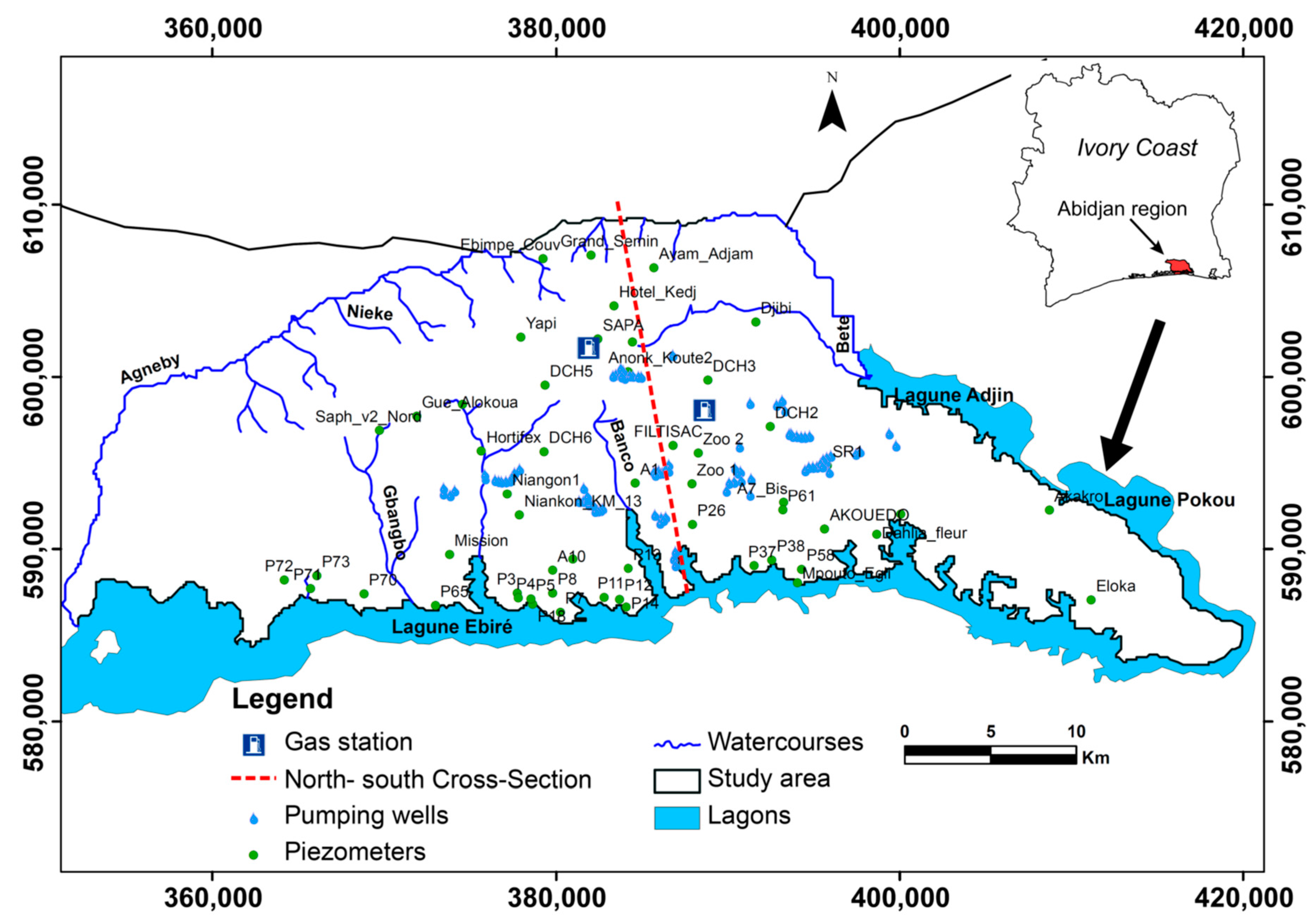
2.1. Location
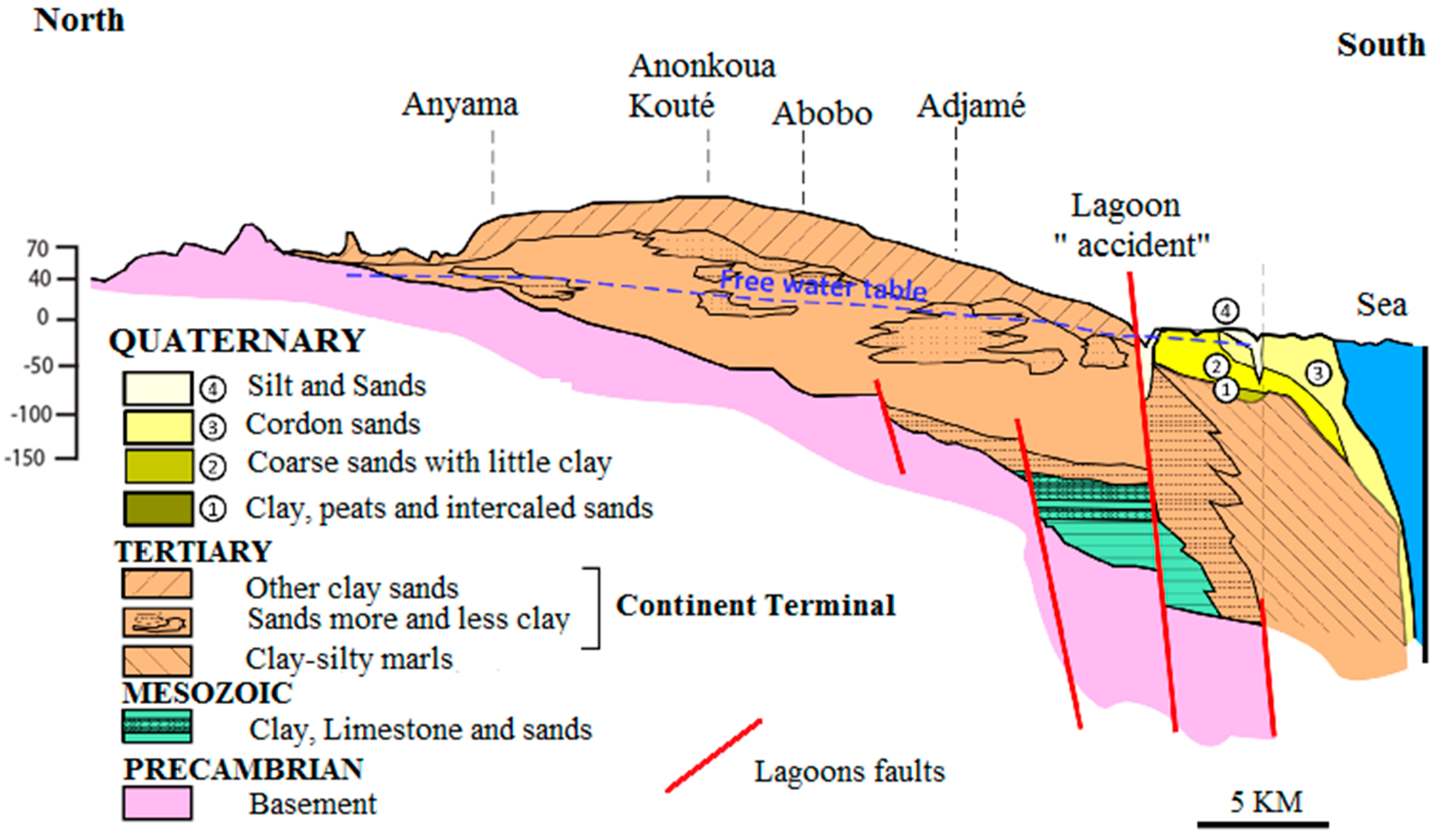
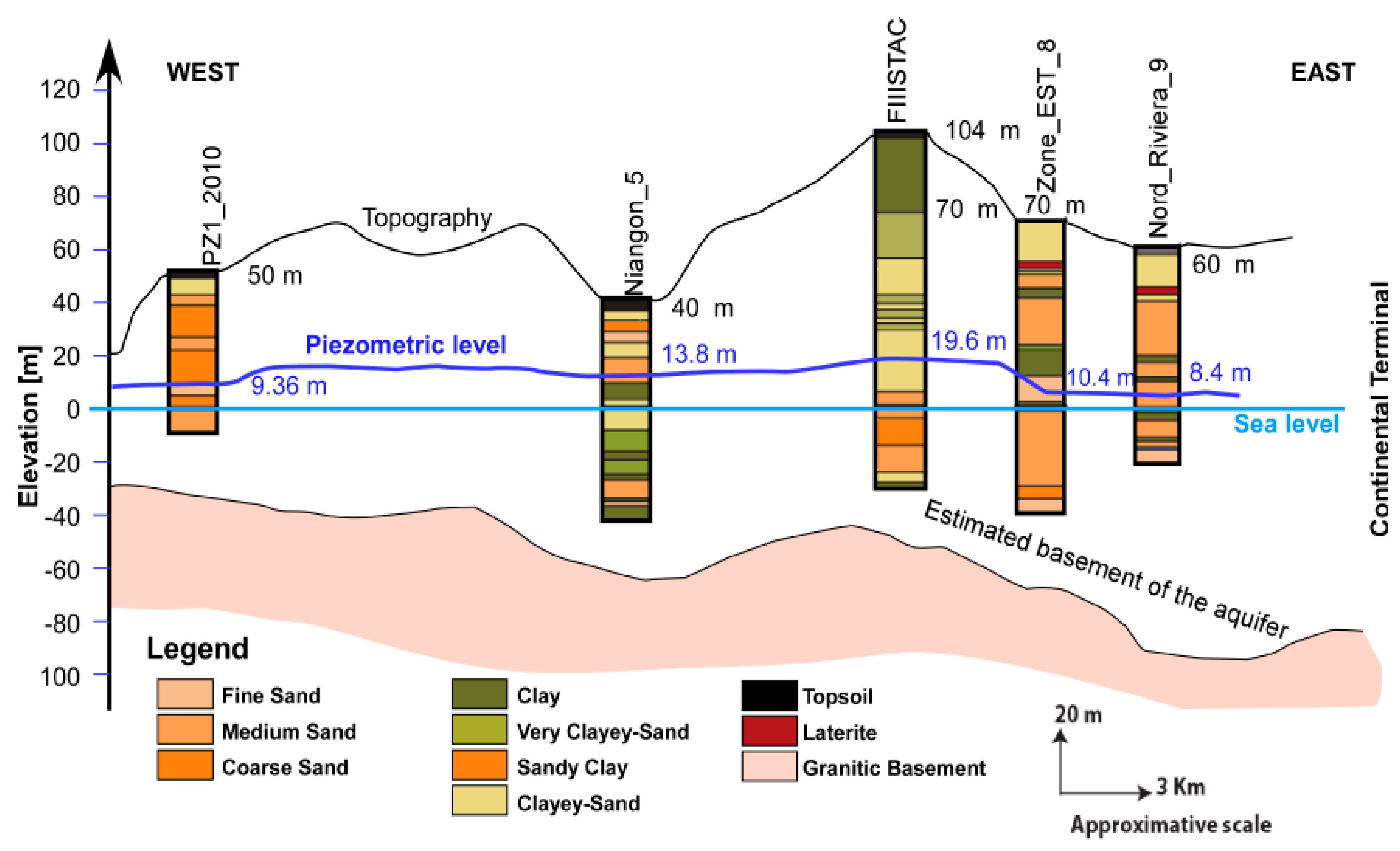
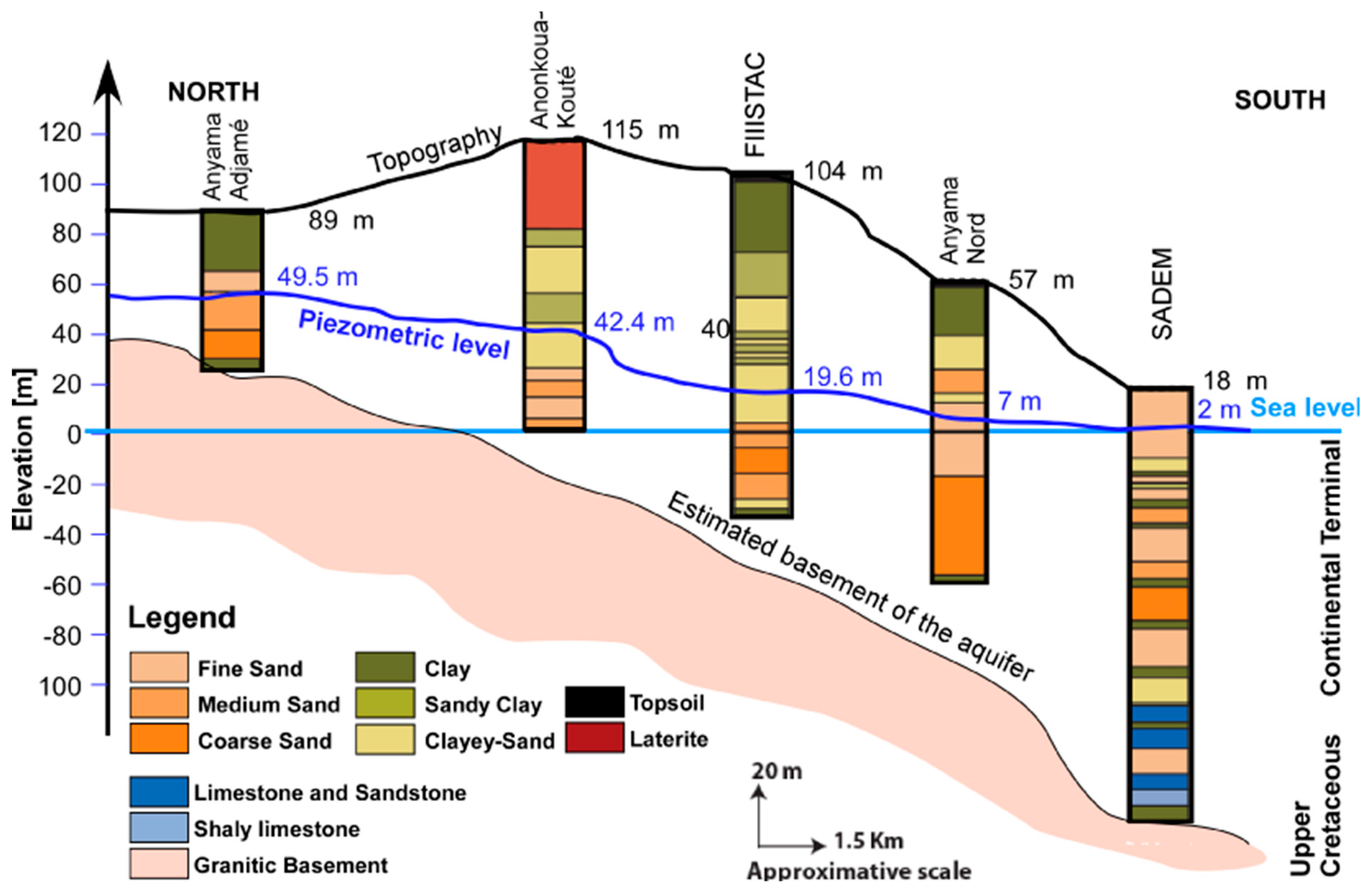
2.2. Geology
2.3. Hydrogeology
3. Materials and Methods
3.1. Layer Properties
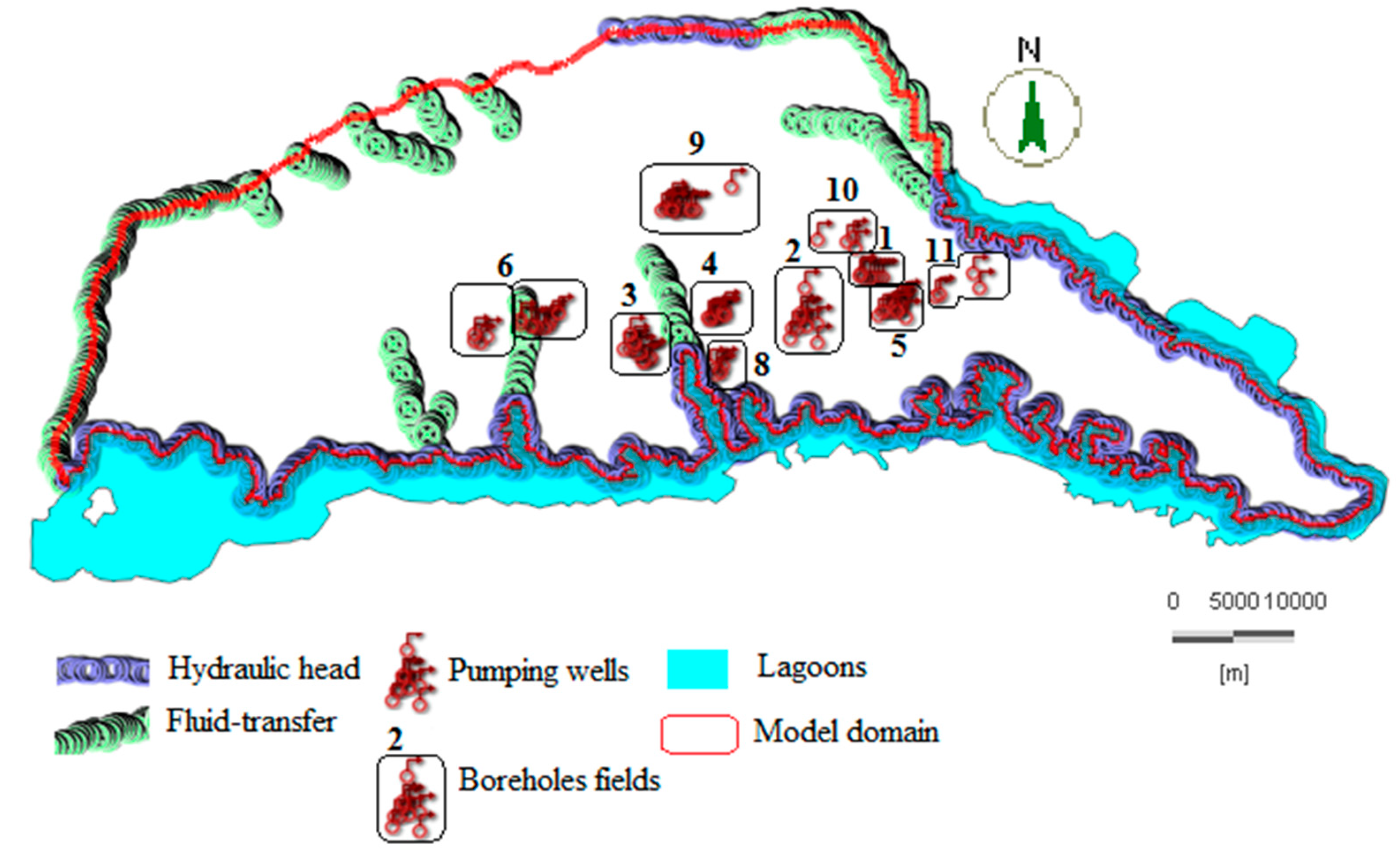
3.2. Boundaries of the Model
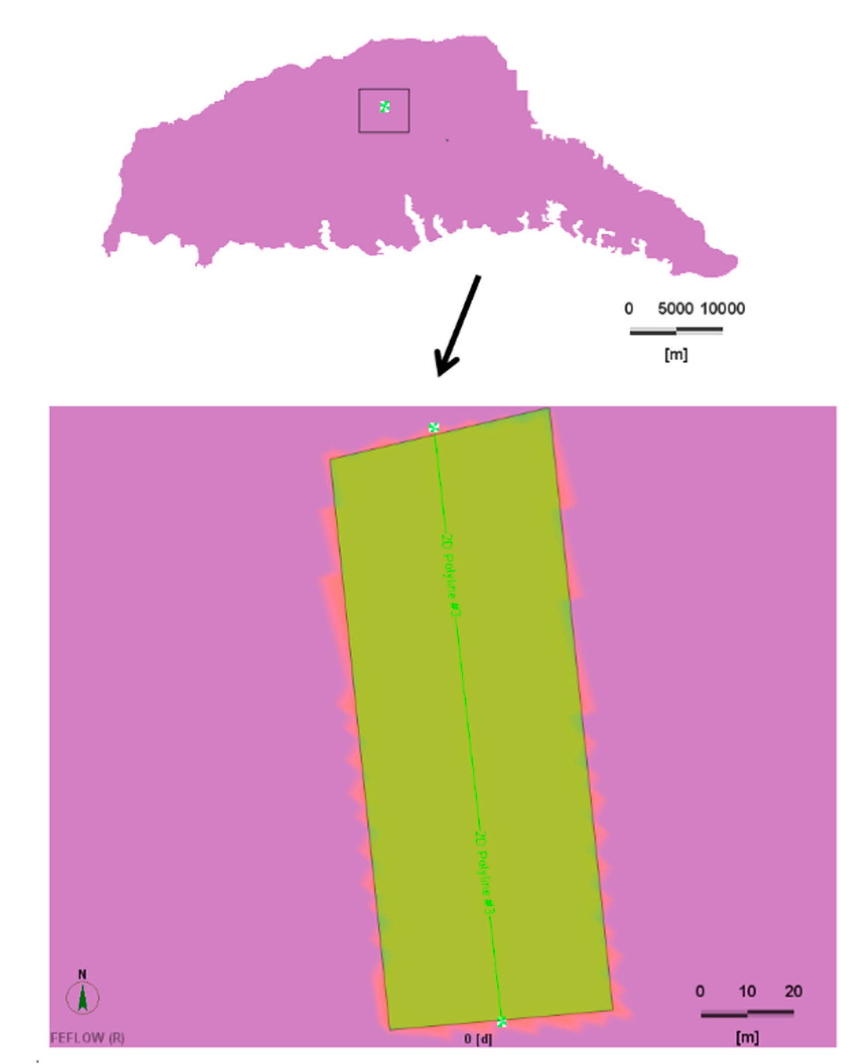
3.2.1. Geographic Boundaries of the Model
3.2.2. Boundary Conditions and Recharge of the Model
3.2.3. Initial Conditions of Underground Flow
4. Results
4.1. Groundwater Flow Model
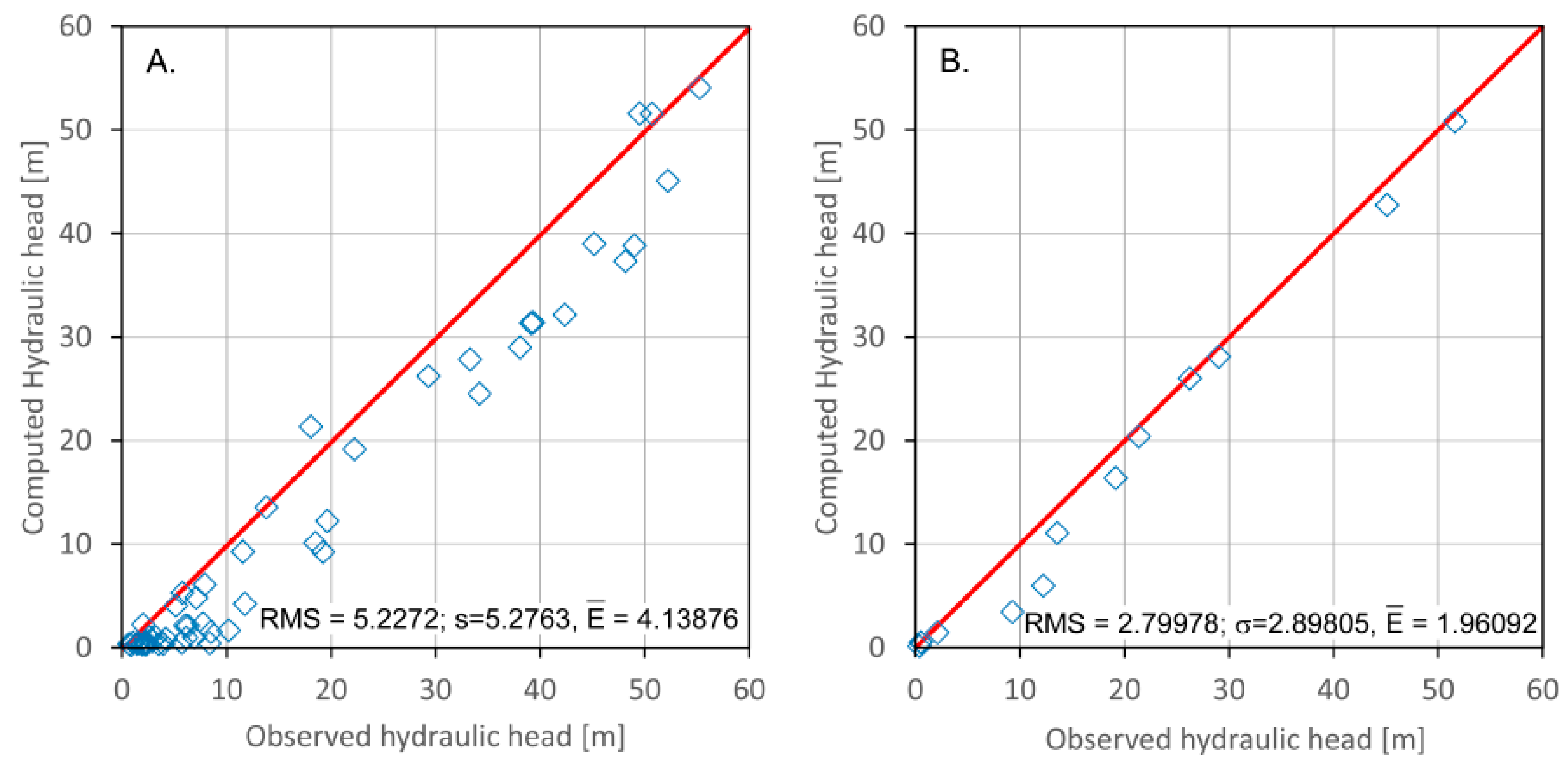
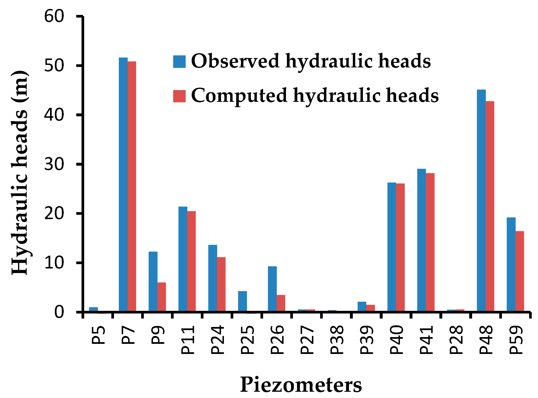
4.1.1. Model Calibration and Validation
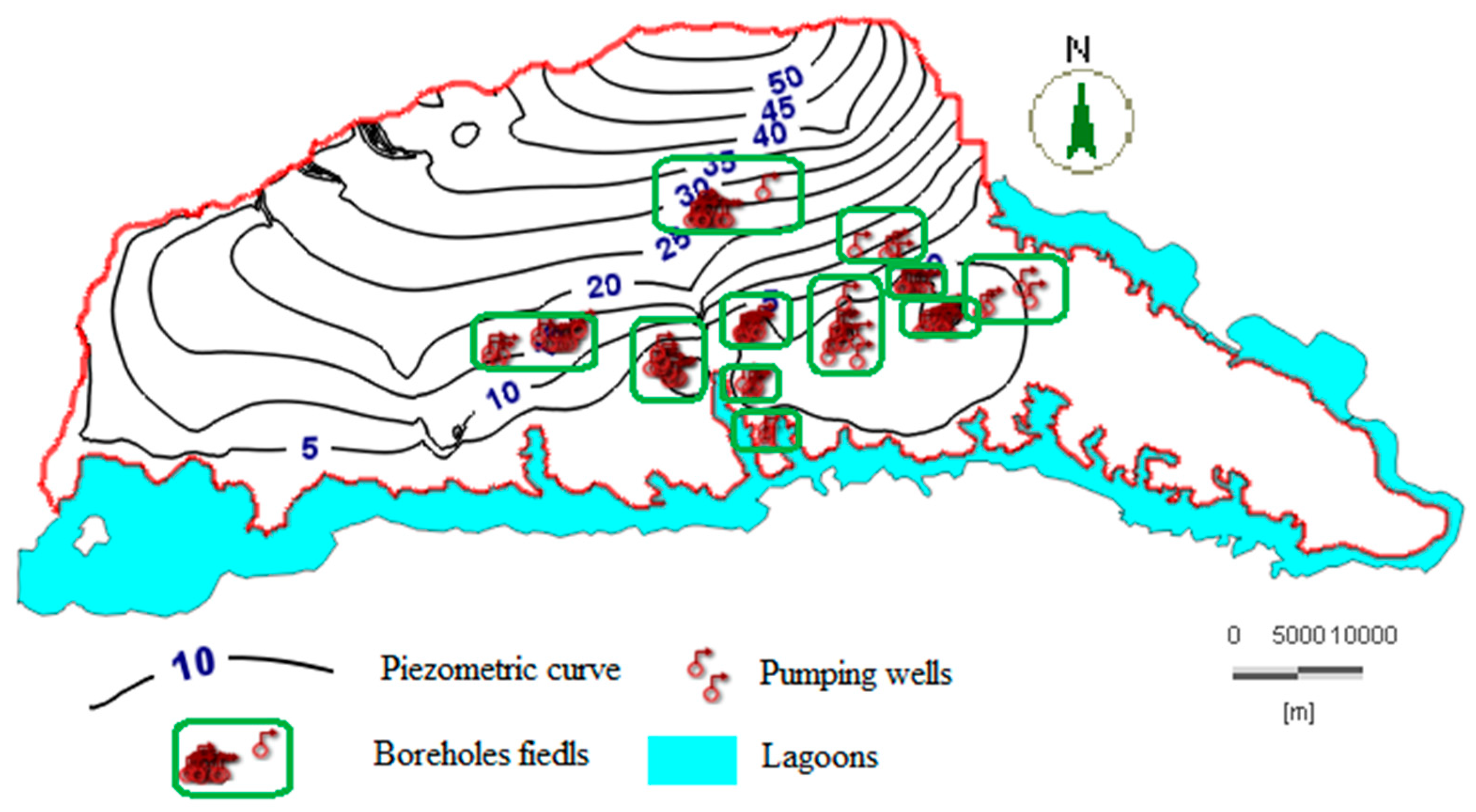
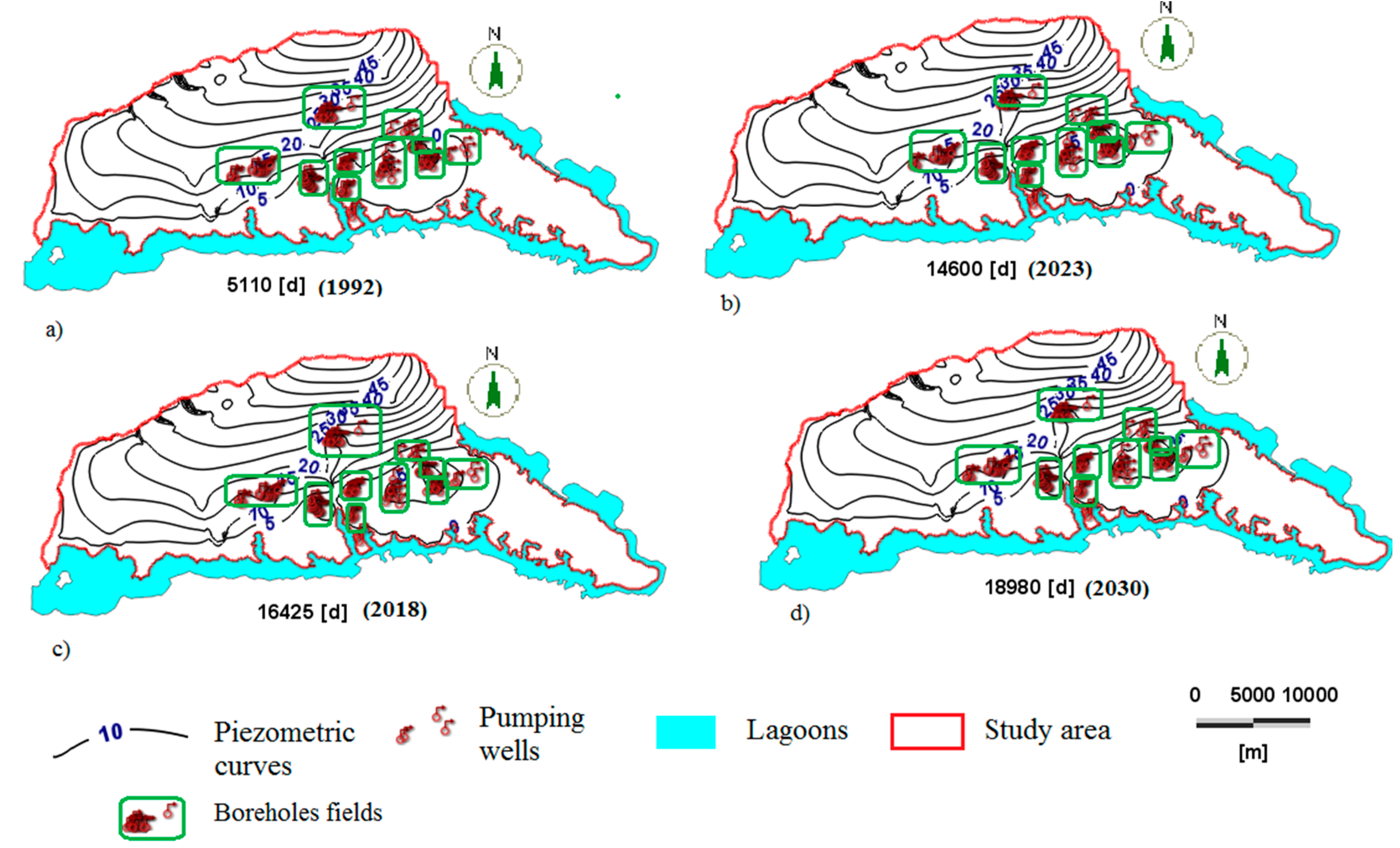
4.1.2. Simulation of the Piezometric Level of the Abidjan Aquifer
4.2. Benzene Transport Simulation
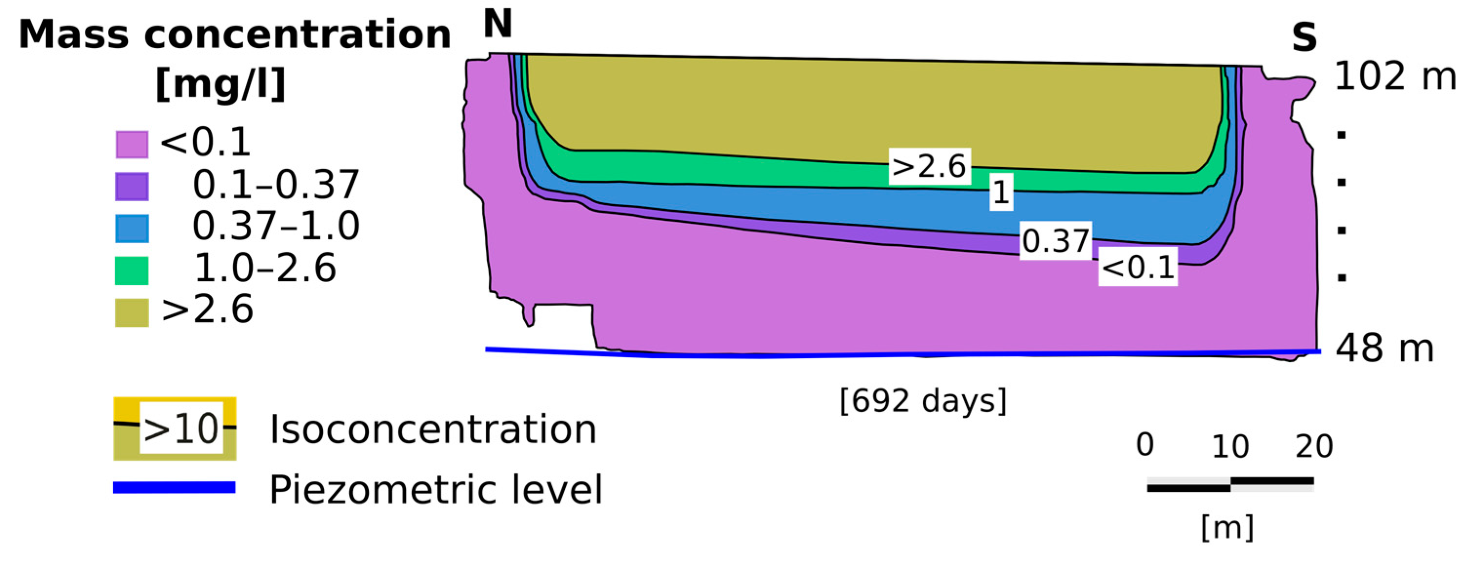
4.2.1. Unsaturated Zone
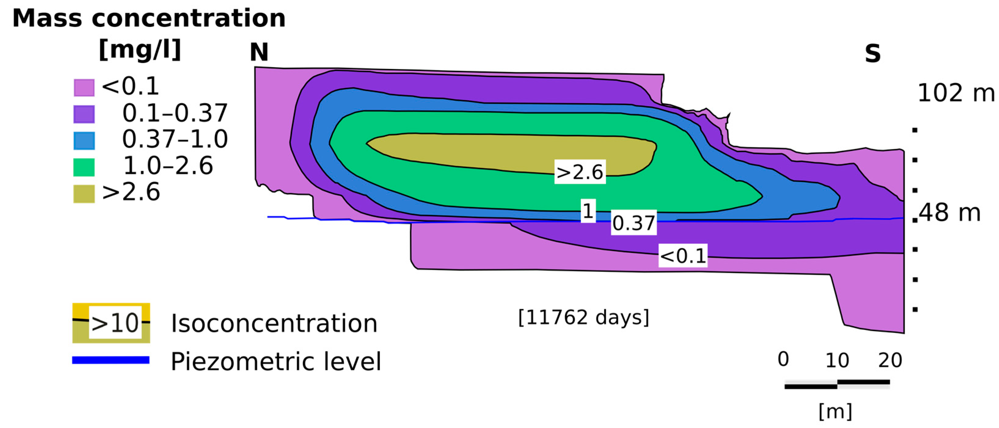
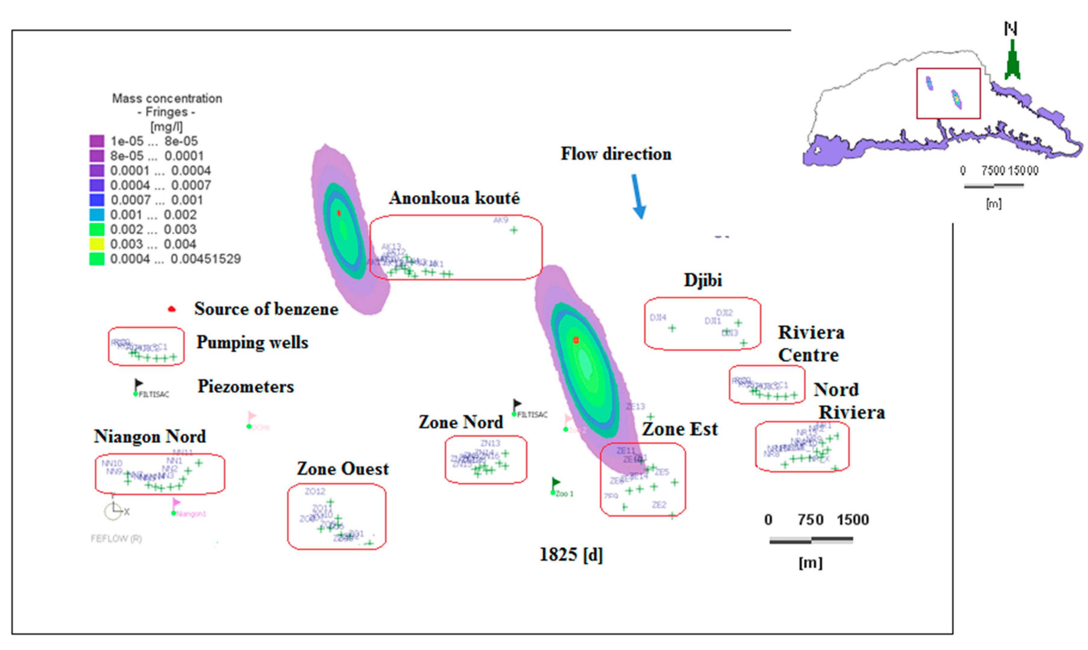
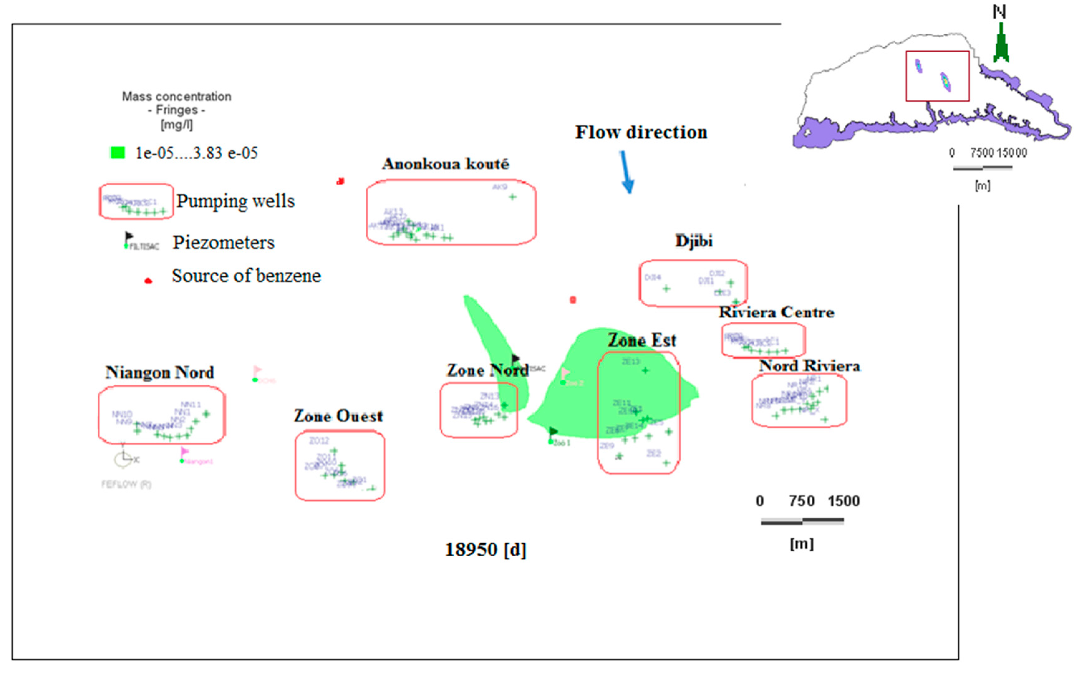
4.2.2. Saturated Zone
4.3. Overall Time and Boreholes Threatened by Pollution
5. Discussion
5.1. Groundwater Flow Model
5.2. Simulation of Transport of Dissolved Benzene in the Unsaturated Zone
5.3. Simulation of the Transport of Dissolved Benzene in the Saturated Zone
5.4. Overall Transport Time of Dissolved Benzene
5.5. Polluted and Threatened Boreholes
5.6. Pollution Issues and Perspectives
6. Conclusions
Author Contributions
Funding
Acknowledgments
Conflicts of Interest
Appendix A

| Boreholes Fields | Designation | Number of Boreholes | Boreholes Name |
|---|---|---|---|
| Zone Nord | ZN | 9 | ZN5, ZN6, ZN8, ZN11, ZN12, ZN13, ZN14, ZN15, ZN16 |
| Anonkoua Kouté | AK | 14 | AK1, AK3, AK4, AK5, AK6, AK7, AK8, AK9, AK10, AK12, AK13, AK15, AK16, AK17 |
| Niangon Nord | NN | 10 | NN1, NN2, NN3, NN4, NN5, NN6, NN7, NN9, NN10, NN11 |
| Zone Ouest | ZO | 11 | ZO1, ZO2, ZO3, ZO4, ZO5, ZO6, ZO7, ZO8, ZO10, ZO11, ZO12 |
| Adjamé Nord | AN | 5 | AN1, AN2, AN7, AN8, AN9 |
| Zone Est | ZE | 11 | ZE1, ZE2, ZE5, ZE7, ZE8, ZE9, ZE10, ZE10, ZE11, ZE13, ZE14 |
| Nord Riviera | NR | 12 | NR1, NR2, NR8, NR9, NR10, NR11, NR12, NR13, NR14, NR16, NR_X, NR_Y |
| Riviera center | RC | 7 | RC1, RC2, RC3, RC4, RC5, RC9, RC8 |
| Plateau | Plateau | 3 | C4, C5, IFAN |
| Djibi | DJI | 4 | DJI1, DJI2, DJI3, DJ4 |
| Niangon2 | N2 | 4 | N2F5, N2F6, N2F7, N2F9 |
| Abata | ABA | 2 | AB1, ABA2, |
| Akandje | AKA | 2 | AKA1, AKA2 |
| Total | 13 | 93 |
| Piezometers | Observed hydraulic heads (m) | Computed hydraulic heads (m) | Difference (m) | Piezometers | Observed hydraulic heads (m) | Computed hydraulic heads (m) | Difference (m) |
|---|---|---|---|---|---|---|---|
| A1 | 7.89 | 6.08 | 1.81 | P14 | 0.84 | 0.23 | 0.61 |
| A10 | 6.04 | 2.14 | 3.90 | P18 | 1.92 | 0.32 | 1.60 |
| A7_Bis | 10.19 | 1.67 | 8.52 | P4 | 2.91 | 0.65 | 2.26 |
| AKOUEDO | 6.13 | 0.98 | 5.15 | P5 | 2.27 | 0.61 | 1.66 |
| Anonk_Koute2 | 42.36 | 32.15 | 10.21 | P65 | 1.05 | 0.50 | 0.55 |
| Ayam_Adjam | 49.52 | 51.60 | −2.08 | P7 | 0.69 | 0.39 | 0.30 |
| Ebimpe_Couv | 50.69 | 51.57 | -0.88 | P70 | 2.01 | 2.24 | -0.23 |
| Filtisac | 19.62 | 12.23 | 7.39 | P72 | 5.16 | 4.09 | 1.07 |
| Grand_Semin | 55.25 | 54.07 | 1.18 | Dahlia_fleur | 3.95 | 0.39 | 3.56 |
| Hortifex | 18.06 | 21.36 | −3.30 | yop_pz_a8 | 6.32 | 2.11 | 4.21 |
| Mission | 5.77 | 5.30 | 0.47 | Saph_v2_Nord | 29.3 | 26.24 | 3.06 |
| Niankon_KM_13 | 11.56 | 9.28 | 2.28 | vp_sodepalm | 38.07 | 29.01 | 9.06 |
| P13 | 1.61 | 0.43 | 1.18 | DCH2 | 18.47 | 10.12 | 8.35 |
| P26 | 6.92 | 1.00 | 5.92 | DCH3 | 34.21 | 24.52 | 9.69 |
| P3 | 4.19 | 0.89 | 3.30 | Djibi | 39.12 | 31.35 | 7.77 |
| P37 | 2.04 | 0.36 | 1.68 | Hotel_Kedj | 52.2 | 45.10 | 7.10 |
| P38 | 1.07 | 0.49 | 0.58 | P71 | 7.73 | 2.36 | 5.37 |
| P58 | 2.61 | 1.04 | 1.57 | P73 | 7.09 | 4.84 | 2.25 |
| P61 | 8.5 | 1.52 | 6.98 | Yapi | 45.16 | 39.02 | 6.14 |
| P8 | 3.26 | 1.01 | 2.25 | SAPA | 49 | 38.85 | 10.15 |
| SR1 | 8.38 | 0.43 | 7.95 | P12 | 2.31 | 0.31 | 2.00 |
| Niangon1 | 13.8 | 13.57 | 0.23 | Mais_Jardin | 5.7 | 0.49 | 5.21 |
| Zoo 1 | 11.75 | 4.24 | 7.51 | Gue_Alokoua | 33.3 | 27.84 | 5.46 |
| Zoo 2 | 19.23 | 9.25 | 9.98 | Mpouto_Egli | 1.42 | 0.37 | 1.05 |
| Akakro | 2.34 | 0.52 | 1.82 | Plantation_Sabo | 48.15 | 37.35 | 10.80 |
| Eloka | 2.2 | 0.50 | 1.70 | DCH5 | 39.33 | 31.41 | 7.92 |
| P11 | 3.51 | 0.36 | 3.15 | DCH6 | 22.22 | 19.16 | 3.06 |
Appendix B
| Years | ||||||||||||||
|---|---|---|---|---|---|---|---|---|---|---|---|---|---|---|
| Boreholes fields | Boreholes name | 1978 | 1978–1980 | 19801–985 | 1985–1992 | 1992–1995 | 1995–2000 | 2000–2005 | 2005–2010 | 2010–2012 | 2012–2015 | 2015–2020 | 2020–2030 | |
| Zone Nord | ZN | Pumping rate (m3/day) | 24000 | 24000 | 30000 | 25824 | 25824 | 32592 | 34992 | 37000 | 37000 | 37000 | 37000 | 37000 |
| Anonkoua Kouté | AK | - | - | 28296 | 21960 | 21960 | 31440 | 38000 | 43000 | 43000 | 43000 | 43000 | 43000 | |
| Niangon Nord | NN | - | - | 28800 | 33000 | 33000 | 40608 | 37000 | 48000 | 48000 | 48000 | 48000 | 48000 | |
| Zone Ouest | ZO | 49200 | 25200 | 31200 | 37488 | 37488 | 37920 | 48000 | 50000 | 50000 | 50000 | 50000 | 50000 | |
| Adjamé Nord | AN | 37680 | 37680 | 31680 | 13848 | 13848 | 20880 | 9300 | 27480 | 27480 | 27480 | 27480 | 27480 | |
| Zone Est | ZE | 29040 | 38304 | 26784 | 28776 | 28776 | 32304 | 33000 | 43992 | 43992 | 43992 | 43992 | 43992 | |
| Nord Riviera | NR | - | - | 36000 | 32496 | 32496 | 33062 | 38000 | 43992 | 43992 | 52790 | 52790 | 52790 | |
| Riviera Center | RC | - | - | 9984 | 16704 | 16704 | 19992 | 20000 | 21288 | 21288 | 21288 | 21288 | 21288 | |
| Plateau | Plateau | 1800 | 30000 | 24000 | 1800 | 1800 | 1368 | 194 | - | - | - | - | - | |
| Djibi | DJI | - | - | - | - | - | - | - | - | 24000 | 24000 | 24000 | 24000 | |
| Niangon2 | N2 | - | - | - | - | - | - | - | - | - | 24000 | 24000 | 24000 | |
| Abatar | ABA | - | - | - | - | - | - | - | - | - | 12000 | 12000 | 12000 | |
| Akandje | AKA | - | - | - | - | - | - | - | - | - | 12000 | 12000 | 12000 | |
References
- Bosca, C. Groundwater law and administration of sustainable development. Medit. Mag. Sci. Train. Technol. 2002, 2, 13–17. [Google Scholar]
- Brassington, R. Field Hydrogeology, 3rd ed.; The Geological Field Guide Series; Prentice Hall: Englewood Cliffs, NJ, USA, 2007; 264p. [Google Scholar]
- Hallam, F.; Acoubi-Khebiza, M.Y.; Oufdou, K.; Oulanouar, M.B. Qualité des eaux souterraines dans une région aride du Maroc: Impact des pollutions sur la biodiversité et relations crustacés—Bactéries d’intérêt sanitaire. Environ. Technol. 2008, 29, 1179–1189. [Google Scholar] [CrossRef] [PubMed]
- Morris, B.L.; Lawrence, A.R.; Chilton, P.J.C.; Adams, B.; Calow, R.C.; Klinck, B.A. A Global Assessment of Problem and Options for Management; United Nations Environment Program Groundwater: Nairobi, Kenya, 2003; 140p. [Google Scholar]
- Abi-Zeid, I. La modélisation Stochastique des Étiages et de Leurs Durées en vue de L’analyse du Risque. Ph.D. Thesis, Université de Québec, Quebec City, QC, Canada, 1997. [Google Scholar]
- Water, U.N. Water in a Changing World: United Nations World Water Development Report 3; World Water Assessment Programme: Paris, France, 2009; Volume 429. [Google Scholar]
- Castany, G. Principes et Méthodes de L’hydrogéologie; Dunod Université: Paris, France, 1982; 238p. [Google Scholar]
- United Nations World Water Assessment Program. WWAP: The 3rd World Water Forum Final Report; United Nations World Water Assessment Program: Kyoto, Japan, 2003; 273p. [Google Scholar]
- Tandia, A.A.; Gaye, C.B.; Faye, A. Origine des teneurs élevées en nitrates dans la nappe phréatique des sables quaternaires de la région de Dakar. Sécheresse 1997, 8, 291–294. [Google Scholar]
- Adelena, S.M. Nitrate pollution of groundwater in Nigeria. In Groundwater Pollution in Africa; CRC Press: Boca Raton, FL, USA, 2006; pp. 37–45. [Google Scholar]
- Takem, G.E.; Chandrasekharam, D.; Ayonghe, P.; Thambidurai, P. Pollution characteristics of alluvial groundwater from springs and bore wells in semi-urban informal settlements of Douala, Cameroon, Western Africa. Environ. Earth Sci. 2010, 61, 287–298. [Google Scholar] [CrossRef]
- Deh, S.K. Contributions de L’évaluation de la Vulnérabilité Spécifique aux Nitrates et d’un Modèle de Transport des Organochlorés à la Protection des Eaux Souterraines du District d’Abidjan (sud de la Côte d’Ivoire). Ph.D. Thesis, Université Félix Houphouet-Boigny, Abidjan, Côte d’Ivoire, 2013; 230p. [Google Scholar]
- Sieczka, A.; Bujakowski, F.; Falkowski, T.; Koda, E. Morphogenesis of a Floodplain as a Criterion for Assessing the Susceptibility to Water Pollution in an Agriculturally Rich Valley of a Lowland River. Water 2018, 10, 399. [Google Scholar] [CrossRef]
- Bugan, R.; Tredoux, G.; Jovanovic, N.; Israel, S. Pollution Plume Development in the Primary Aquifer at the Atlantis Historical Solid Waste Disposal Site, South Africa. Geosciences 2018, 8, 231. [Google Scholar] [CrossRef]
- Koda, E.; Sieczka, A.; Osinski, P. Ammonium Concentration and Migration in Groundwater in the Vicinity of Waste Management Site Located in the Neighborhood of Protected Areas of Warsaw, Poland. Sustainability 2016, 8, 1253. [Google Scholar] [CrossRef]
- Václavík, V.; Ondrašiková, I.; Dvorský, T.; Černochová, K. Leachate from Municipal Waste Landfill and Its Natural Degradation—A Case Study of Zubří, Zlín Region. Int. J. Environ. Res. Public Health 2016, 13, 873. [Google Scholar] [CrossRef]
- Howard, G.; Bartram, J.; Pedley, S.; Schmoll, O.; Chorus, I.; Berger, P. Chapter 1: Groundwater and public health. In Protecting Groundwater for Health: Managing the Quality of Drinking-Water Sources; London IWA Publishing: London, UK, 2006; pp. 3–20. [Google Scholar]
- Xu, Y.; Usher, B.H. Issues of groundwater pollution in Africa. In Groundwater pollution in Africa; CRC Press: Boca Raton, FL, USA, 2006; pp. 3–9. [Google Scholar]
- Kouamé, K.J. Contribution à la Gestion Intégrée des Ressources en Eaux (GIRE) du District d’Abidjan (Sud de la Côte d’Ivoire): Outils d’aide à la Décision pour la Prévention et la Protection des Eaux Souterraines Contre la Pollution. Ph.D. Thesis, Université de Cocody, Abidjan, Côte d’Ivoire, 2007; 229p. [Google Scholar]
- Institut National de la Statistique (INS). Recensement Général de la Population et de l’Habitation (RGPH). Données Socio-Démographiques et Économiques des Localités, Résultats Définitifs par Localités, Région des Lagunes; INS: Abidjan, Côte d’Ivoire, 2014; 26p. [Google Scholar]
- Direction de l’Hydraulique Humaine en Côte d’Ivoire; Ministère des Infrastructures Economiques: Abidjan, Côte d’Ivoire, 2001; 66p.
- Société de Distribution d’Eau en Côte d’Ivoire (SODECI). Etude de la Gestion et de la Protection de la Nappe d’Abidjan; Actualisation des études hydrogéologiques SOGREHAH de 1997; SODECI: Abidjan, Côte d’Ivoire, 2015; 78p. [Google Scholar]
- Dongo, K.; Tiembre, I.; Kone, B.A.; Zurbrugg, C.; Odrematt, P.; Tanner, M.; Zinsstag, J.; Cissé, G. Exposure to toxic waste containing high concentrations of hydrogen sulphide illegally dumped in Abidjan. Environ. Sci. Pollut. Resour. 2012, 10, 3192–3199. [Google Scholar] [CrossRef]
- Jourda, J.P. Contribution à L’étude Géologique et Hydrogéologique de la Région du Grand Abidjan (Côte D’Ivoire). Ph.D. Thesis, Université Scientifique, Technique et Médicale de Grenoble, Grenoble, France, 1987; 319p. [Google Scholar]
- Adiaffi, B. Apport de la Géochimie Isotopique, de L’hydrochimie et de la Télédétection à la Connaissance des Aquifères de la Zone de Contact « Socle-Bassin Sédimentaire » du Sud-Est de la Côte d’Ivoire. Ph.D. Thesis, Université Paris-Sud, Orsay, France, 2008; 196p. [Google Scholar]
- Gilli, E.; Mangan, C.; Mudry, J. Hydrogéologie: Objets, Méthodes, Applications, 3rd ed.; Dunod: Paris, France, 2012; 340p. [Google Scholar]
- Jourda, J.P.; Kouamé, K.J.; Saley, M.B.; Kouadio, B.H.; Oga, Y.S. Contamination of the Abidjan aquifer by sewage: An assessment of extent and strategies for protection. In Groundwater Pollution in Africa; CRC Press: Boca Raton, FL, USA, 2006; pp. 291–300. [Google Scholar]
- Kouamé, K.I. Pollution Physico-Chimique des Eaux dans la Zone de la Décharge d’Akouédo et Analyse du Risque de Contamination de la Nappe d’Abidjan par un Modèle de Simulation des Écoulements et du Transport des Polluants, Ph.D. Thesis, Université d’Abobo-Adjamé, Abidjan, Côte d’Ivoire, 2007; 206p. [Google Scholar]
- Dongo, K.; Kouamé, K.F.; Koné, B. Analyse de la situation de l’environnement sanitaire des quartiers défavorisés dans le tissu urbain de Yopougon à Abidjan, Côte d’Ivoire. Vertigo-Rev. Electron. Sci. Environ. 2008, 8, 17. [Google Scholar] [CrossRef]
- Soro, N.; Ouattara, L.; Dongo, K.; Kouadio, K.E.; Ahoussi, K.E.; Soro, G.; Oga, M.S.; Savané, I.; Biémi, J. Déchets municipaux dans le District d’Abidjan en Côte d’Ivoire sources potentielles de pollution des eaux souterraines. Int. J. Biol. Chem. Sci. 2010, 4, 364–384. [Google Scholar] [CrossRef]
- Guiraud, R. L’hydrogéologie de l’Afrique. J. Afr. Sci. 1988, 7, 519–543. [Google Scholar] [CrossRef]
- Soro, N.C. Géolocalisation des Stations D’essences dans la Commune D’Abobo. Master’s Thesis, Université Félix Houphouët-Boigny, Abidjan, Côte d’Ivoire, 2015. [Google Scholar]
- Fiche de Données Toxicologiques et Environnementales des Substances Chimiques. Available online: https://substances.ineris.fr/fr/page/21 (accessed on 26 January 2019).
- Institut National de Statistiques. Recensement Général de la Population et de l’Habitation de la Côte d’Ivoire (RGPH). Données Socio-Démographiques et Économiques des Localités, Résultats Définitifs par Localités, Région des Lagunes; Institut National de Statistiques: Abidjan, Côte d’Ivoire, 2001; Volume 3, p. 43. [Google Scholar]
- Martin, L. Morphologie, Sédimentologie et Paléogéographie au Quaternaire récent du Plateau Continental Ivoirien. Ph.D. Thesis, Université de Paris VI, Paris, France, 1973; 340p. [Google Scholar]
- Tastet, J.P. Environnements Sédimentaires et Structuraux Quaternaires du Littoral du Golfe de Guinée (Côte d’Ivoire, Togo, Bénin). Ph.D. Thesis, Université de Bordeaux 1, Bordeaux, France, 1979; 181p. [Google Scholar]
- Aghui, N.; Biemi, J. Géologie et hydrogéologie des nappes de la région d’Abidjan et risques de contamination. Ann. l’Université Natl. Côte d’Ivoire 1984, 20, 331–347. [Google Scholar]
- Delor, C.; Diaby, I.; Siméon, Y.; Yao, B.; Tastet, J.P.; Vidal, M.; Chiron, J.P.; Dommang, A. Notice Explicative de la Carte Géologique de la Côte d’Ivoire à 1/200000; Mémoire de la Direction de la Géologie de Côte d’Ivoire, n 3: Abidjan, Côte d’Ivoire, 1992a; 26p. [Google Scholar]
- Delor, C.; Diaby, I.; Siméon, Y.; Yao, B.; Tastet, J.P.; Vidal, M.; Chiron, J.P.; Dommang, A. Notice Explicative de la Carte Géologique de la Côte d’Ivoire à 1/200000; Mémoire de la Direction de la Géologie de Côte d’Ivoire, n 4: Abidjan, Côte d’Ivoire, 1992b; 30p. [Google Scholar]
- Loroux, B.F.E. Contribution à L’étude Hydrogéologique du Bassin Sédimentaire de Côte d’Ivoire. Ph.D. Thesis, Université de Bordeaux I, Bordeaux, France, 1978; 93p. [Google Scholar]
- Ashraf, A.; Ahmad, Z. Regional groundwater flow modelling of Upper Chaj Doab of Indus Basin, Pakistan using finite element model (Feflow) and geoinformatics. Geophys. J. Int. 2008, 173, 17–24. [Google Scholar] [CrossRef] [Green Version]
- Thangarajan, M.; Rajan, T. Regional Groundwater Modeling; Capital Publishing Company: New Delhi, India, 2004; Volume 340. [Google Scholar]
- Hiscock, K.M.; Bense, V.F. Hydrogeology: Principes and Practice, 2nd ed.; Wiley and Sons: Hoboken, NJ, USA, 2014; 519p. [Google Scholar]
- Yeh, T.-C.J.; Khaleel, R.; Carroll, K.C. Flow through Heterogeneous Geologic Media; Cambridge University Press: Cambridge, UK, 2015; 243p. [Google Scholar]
- Anderson, M.P.; Woessner, W.W.; Hunt, R.J. Applied Groundwater Modelling: Simulation of Flow and Advective Transport, 2nd ed.; Elsevier Inc.: New York, NY, USA, 2015; 564p. [Google Scholar]
- Bear, J. Dynamics of Fluids in Porous Media; Elsevier: New York, NY, USA, 1972; 764p. [Google Scholar]
- Ingebritsen, S.; Sanford, W.; Neuzil, C. Groundwater in Geologic Processes, 2nd ed.; Cambridge University Press: Cambridge, UK, 2006; 536p. [Google Scholar]
- Fitts, C.R. Groundwater Sciences, 2nd ed.; Elsevier, Academy press: Waltham, MA, USA, 2013; 672p. [Google Scholar]
- Diersch, H.-J.G. Feflow, Finite element Modelling of Flow, Mass and Heat Transport in Porous and Fractured Media; Springer Science & Business Media: Berlin, Germany, 2014; 996p. [Google Scholar]
- Sylla, M.B.; Pal, J.S.; Faye, A.; Dimobe, K.; Kuntsmann, H. Climate change to severely impact West African basin scale irrigation in 2 °C and 1.5 °C global warming scenarios. Nat. Sci. Rep. 2018, 8, 14395. [Google Scholar] [CrossRef] [PubMed]
- Société Grenobloise d’Etudes et d’Applications Hydrauliques (SOGREAH). Etude de la Gestion et de la Protection de la Nappe Assurant la Production en eau Potable d’Abidjan. Etude sur Modèle Mathématique. Rapport Rapport de Phase 2; Présentation du modèle mathématique et des résultats du calage; Ministère des Infrastructures Economiques, Direction et Contrôles des Grands Travaux (DCGTX); Société Grenobloise d’Etudes et d’Applications Hydrauliques (SOGREAH): Lyon, France, 1996; 30p. [Google Scholar]
- Kouassi, K.A. Modélisation en Milieu Poreux Saturé par Approche Inverse via une Paramétrisation Multi-Échelle: Cas de L’aquifère du Continental Terminal. Ph.D. Thesis, Université Nangui-Abrogoua, Abidjan, Côte d’Ivoire, 2013; 268p. [Google Scholar]
- Van Genuchten, M.T. A closed-form Equation for Predicting the Hydraulic Conductvity of Unsaturated soils. Sci. Soc. Am. J. 1980, 44, 892–898. [Google Scholar] [CrossRef]
- Ippisch, O.; Vogel, H.J.; Bastian, P. Validity limits for the van Genuchten–Mualem model and implications for parameter estimation and numerical simulation. Adv. Water. Resour. 2006, 29, 1780–1789. [Google Scholar] [CrossRef]
- Ghanbarian, A.B.; Liaghat, A.; Huang, G.-H.; Van Genuchten, M.T. Estimation of the van Genuchten Soil Water Retention Properties from Soil Textural Data. Soil Sci. Soc. China 2010, 20, 456–465. [Google Scholar]
- Mobile Geochemistry Incorporation. Available online: http://www.handpmg.com/articles/lustline29-oh-henry.html (accessed on 12 January 2018).
- Matti, B.; Tacher, L. Modèles couplés hydraulique/thermique de la nappe alluviale de la plaine du Rhône et modélisation de l’implantation d’un système de refroidissement eau-eau à l’hôpital cantonal de Sion (VS, Suisse). Swiss Bull. Angew. Geol. 2009, 14, 47–64. [Google Scholar]
- Wiedemeieir, T.H.; Swanson, M.A.; Wilson, J.T.; Kampell, D.H.; Miller, R.N.; Hansen, J.E. Approximation of biodegradation rate constants for monoaromatic hydrocarbons (BTEX) in ground water. Groundw. Monit. Remediat. 1996, 16, 186–194. [Google Scholar] [CrossRef]
- Rasmussen, H.; Rouleau, A. Guide de Détermination D’aires d’alimentation et de Protection de Captage D’eaux Souterraines. Centre D’étude sur les Ressources Minérales, Université de Québec à Chicoutimi. Contrat du Ministère de L’environnement du Québec 2003. Available online: https://www.agrireseau.net/agroenvironnement/documents/guide.pdf (accessed on 12 December 2017).
- Gomez, D.E.; Alvarez, P.J.J. Modeling the natural attenuation of benzene in groundwater impacted by ethanol-blended fuels: Effect of ethanol content on the lifespan and maximum length of benzene plumes. Water Resour. 2009, 45, W03409. [Google Scholar] [CrossRef]
- Adams, J.A.; Reddy, K.A. Removal of dissolved- and free-phase benzene pools from ground water using in situ air sparging. J. Environ. Eng. 2000, 126, 697–707. [Google Scholar] [CrossRef]
- Leblanc, Y. Prédiction de l’effet du décapage d’une mine à ciel ouvert sur l’hydrogéologie locale à l’aide de la modélisation numérique systèmes geost. Int. Laval Qué. 1999, 2, 3. [Google Scholar]


| Borehole Fields | Designation | Pumping Rate (m3/day) | Number of Boreholes |
|---|---|---|---|
| Zone Nord | ZN | 13,992 | 2 |
| Anonkoua Kouté | AK | 0 | 0 |
| Niangon Nord | NN | 0 | 0 |
| Zone Ouest | ZO | 46,536 | 8 |
| Adjamé Nord | AN | 24,696 | 5 |
| Zone Est | ZE | 44,112 | 7 |
| Nord Riviera | NR | 30,168 | 5 |
| Riviera Center | RC | 0 | 0 |
| Plateau | Plateau | 18,000 | 3 |
| Djibi | DJI | 0 | 0 |
| Niangon2 | N2 | 0 | 0 |
| Abata | ABA | 0 | 0 |
| Akandje | AKA | 0 | 0 |
| Total | 6 | 177,504 | 30 |
| × 103 m3/j | Rate in | Rate out | Difference | |
|---|---|---|---|---|
| Imposed heads | Dirichlet | 39 | 332 | −292 |
| Cauchy | 229 | 144 | 86 | |
| Pumping wells | 0 | 356 | −356 | |
| Recharge | 542 | 0 | 542 | |
| Storage capture | 21 | 0 | 21 | |
| Imbalance | 831 | 832 | 1 | |
| Piezometers Name | Simulation (years) | Drawdown of the Water Table (m) | |||||
|---|---|---|---|---|---|---|---|
| 1978 | 1992 | 2018 | 2023 | 2030 | |||
| AKOUEDO | Simulated hydraulic heads (m) | 0.98 | −0.53 | −1.43 | −1.63 | −1.70 | 2.68 |
| Ayam_Adjam | 51.6 | 50.81 | 50.14 | 50.08 | 50.00 | 1.60 | |
| Filtisac | 12.23 | 5.99 | 3.22 | 2.49 | 2.10 | 10.13 | |
| Hortifex | 21.36 | 20.41 | 19.82 | 19.76 | 19.73 | 1.63 | |
| Niangon1 | 13.57 | 11.08 | 10.50 | 10.48 | 10.46 | 3.11 | |
| Zoo 1 | 4.24 | −0.32 | −2.07 | −2.60 | −2.85 | 7.09 | |
| Zoo 2 | 9.25 | 3.47 | 0.82 | 0.03 | −0.36 | 9.61 | |
| Akakro | 0.52 | 0.51 | 0.50 | 0.50 | 0.50 | 0.02 | |
| Dahlia_fleur | 0.39 | 0.15 | −0.05 | −0.09 | −0.10 | 0.49 | |
| yop_pz_a8 | 2.11 | 1.47 | 1.35 | 1.34 | 1.34 | 0.77 | |
| Saph_v2_Nord | 26.24 | 26.03 | 25.63 | 25.52 | 25.46 | 0.78 | |
| vp_sodepalm | 29.01 | 28.13 | 27.41 | 27.27 | 27.19 | 1.82 | |
| Eloka | 0.5 | 0.50 | 0.50 | 0.50 | 0.50 | 0.00 | |
| Hotel_Kedj | 45.1 | 42.77 | 40.81 | 40.64 | 40.46 | 4.64 | |
| DCH6 | 19.16 | 16.39 | 15.42 | 15.32 | 15.25 | 3.91 | |
| Parameters | Layer 1 Clayey Sand | Layer 2 Medium Sand | Layer 3 Coarse Sand |
|---|---|---|---|
| Hydraulic conductivity (m/s) | Kxx = Kyy = 7Kzz 1 × 10⁻⁴ | Kxx = Kyy = 7Kzz 3 × 10⁻⁴ | Kxx = Kyy = 7Kzz 4 × 10⁻⁴ |
| Porosity [-] | 0.18 | 0.2 | 0.25 |
| Recharge [mm/year] | 200250 | ||
| 1Maximal saturation Ss [-] | 0.5 | 0.9 | 1 |
| 1Residual saturation Sr [-] | 0.1 | 0.2 | 0.25 |
| 1α [1/m] | 0.0135 | 0.0135 | 0.0135 |
| 1n [-] | 1.08 | 1.08 | 1.08 |
| 1Henry’s constant KH [-] | 0.25 | ||
| 1Molecular diffusion coefficient [m2/s] | 5 × 10⁻⁹ | ||
| 1Decay rate [1/j] | 0.002 | ||
| Unsaturated zone | Saturated zone | ||
| Longitudinal dispersivity [m] | e/10 | L/10 | |
| Transverse dispersivity [m] | e/100 | L/100 | |
| Unsaturated zone thickness [m] | 56 (N’Dotré) and 88 (Anador) | - | |
| Average distance [m] | - | 5000 | |
| Concentration [mg/L] | 43.12 14.37 | 0.37 | |
| Boreholes | Detected Concentration (mg/L) | ||||||
|---|---|---|---|---|---|---|---|
| 8 × 10⁻⁵ | 7 × 10⁻⁴ | 8 × 10⁻⁴ | 9 × 10⁻⁴ | 0.001 | 0.0011 | ||
| ZE11 | Time (days) | 2190 | 3650 | 3900 | 4015 | 4380 | 5475 |
| ZE10 | 2555 | 4380 | 5110 | - | - | - | |
| ZE1 | 3650 | - | - | - | - | - | |
| ZE13 | 3650 | - | - | - | - | - | |
| ZE7 | 4015 | - | - | - | - | - | |
| Boreholes | Concentrations (mg/L) | ||||||
|---|---|---|---|---|---|---|---|
| 8 × 10⁻⁵ | 7 × 10⁻⁴ | 8 × 10⁻⁴ | 9 × 10⁻⁴ | 0.001 | 0.0011 | ||
| ZE11 | Time | 38 years and two months | 42 years and two months | 42 years and 11 months | 43 years and two months | 44 years and two months | 47 years and two months |
| ZE10 | 39 years and two months | 44 years and two months | 46 years and two months | - | - | - | |
| ZE1 | 42 years and two months | - | - | - | - | - | |
| ZE13 | 42 years and two months | - | - | - | - | - | |
| ZE7 | 43 years and two months | - | - | - | - | - | |
© 2019 by the authors. Licensee MDPI, Basel, Switzerland. This article is an open access article distributed under the terms and conditions of the Creative Commons Attribution (CC BY) license (http://creativecommons.org/licenses/by/4.0/).
Share and Cite
Kouamé, A.A.; Jaboyedoff, M.; Goula Bi Tie, A.; Derron, M.-H.; Kouamé, K.J.; Meier, C. Assessment of the Potential Pollution of the Abidjan Unconfined Aquifer by Hydrocarbons. Geosciences 2019, 9, 60. https://doi.org/10.3390/geosciences9020060
Kouamé AA, Jaboyedoff M, Goula Bi Tie A, Derron M-H, Kouamé KJ, Meier C. Assessment of the Potential Pollution of the Abidjan Unconfined Aquifer by Hydrocarbons. Geosciences. 2019; 9(2):60. https://doi.org/10.3390/geosciences9020060
Chicago/Turabian StyleKouamé, Amenan Agnès, Michel Jaboyedoff, Albert Goula Bi Tie, Marc-Henri Derron, Kan Jean Kouamé, and Cédric Meier. 2019. "Assessment of the Potential Pollution of the Abidjan Unconfined Aquifer by Hydrocarbons" Geosciences 9, no. 2: 60. https://doi.org/10.3390/geosciences9020060