Evaluating GRACE Mass Change Time Series for the Antarctic and Greenland Ice Sheet—Methods and Results

Abstract

Satellite gravimetry data acquired by the Gravity Recovery and Climate Experiment (GRACE) allows to derive the temporal evolution in ice mass for both the Antarctic Ice Sheet (AIS) and the Greenland Ice Sheet (GIS). Various algorithms have been used in a wide range of studies to generate Gravimetric Mass Balance (GMB) products. Results from different studies may be affected by substantial differences in the processing, including the applied algorithm, the utilised background models and the time period under consideration. This study gives a detailed description of an assessment of the performance of GMB algorithms using actual GRACE monthly solutions for a prescribed period as well as synthetic data sets. The inter-comparison exercise was conducted in the scope of the European Space Agency’s Climate Change Initiative (CCI) project for the AIS and GIS, and was, for the first time, open to everyone. GMB products generated by different groups could be evaluated and directly compared against each other. For the period from 2003-02 to 2013-12, estimated linear trends in ice mass vary between −99 Gt/yr and −108 Gt/yr for the AIS and between −252 Gt/yr and −274 Gt/yr for the GIS, respectively. The spread between the solutions is larger if smaller drainage basins or gridded GMB products are considered. Finally, findings from the exercise formed the basis to select the algorithms used for the GMB product generation within the AIS and GIS CCI project.

1. Introduction

The Climate Change Initiative (CCI) programme, set up by the European Space Agency (ESA), aims at the provision of reliable, long-term, satellite-based data products to investigate and manage climate change [1]. Data products are provided for a number of so-called Essential Climate Variables (ECV), which include the Greenland Ice Sheet (GIS) and the Antarctic Ice Sheet (AIS). The Antarctic Ice Sheet CCI project (AIS_cci) and the Greenland Ice Sheet CCI project (GIS_cci) deliver different ECV parameters for their respective ice sheets, e.g., surface elevation change, ice flow velocity, grounding line location and ice sheet mass balance.

A user survey, performed within a precursor study of the AIS_cci project, indicates that ice sheet mass balance is one of the most important data products required by the scientific community [2]. Launched in 2002 and operational until 2017, the Gravity Recovery and Climate Experiment (GRACE) was the only space-borne sensor designed to directly observe mass redistribution [3]. Hence, GRACE satellite gravimetry data are most suitable to infer mass balance products. Two different types of Gravimetric Mass Balance (GMB) products are provided by the CCI ice sheets projects: (1) time series of monthly mass changes for the entire ice sheets and individual drainage basins, describing the evolution in ice mass (GMB basin product), and (2) time series of monthly mass change grids covering the entire ice sheet (GMB gridded product), both relative to an arbitrary reference value. Both GMB products are described in detail in the corresponding product user guide [4,5].

GRACE Level-2 products include monthly sets of spherical harmonic coefficients of the Earth’s gravity field (Stokes coefficients). They are affected by spatially correlated errors, typically visible in terms of north-south orientated stripes in the spatial domain. These error effects require an appropriate post-processing as a part of GRACE analysis for mass change studies. Proposed filtering approaches suitable to reduce GRACE errors comprise simple isotropic Gaussian filters [6] as well as methods accounting for the anisotropic nature of the GRACE errors (e.g., [7,8]). The GRACE error characteristics imply a limited spatial resolution of 200–500 km, depending on the geographical location, temporal scale, and other factors. Mass changes cannot be resolved with higher spatial resolution due to the attenuation of the corresponding small-scale gravity changes at satellite altitude. This hinders the separation of nearby mass changes. The resulting error is known as leakage error and may be increased by the application of a filtering technique [6]. Hence, an algorithm used to derive GMB products needs to efficiently damp GRACE errors while retaining the geophysical signal and reducing signal leakage.

A wide range of studies made use of GRACE-derived time-variable gravity field solutions to investigate the spatial and temporal evolution of ice sheet mass. Results from these studies are difficult to compare due to differences in the period under investigation [9], the utilised Level-2 products [10], the model used to correct for solid Earth mass changes (i.e., glacial isostatic adjustment—GIA) [11] and the algorithm applied in the mass change inference. Even in the event of identical input data, differences caused by the algorithms’ ability to reduce both GRACE errors and signal leakage remain. A widely used method makes use of the regional integration approach, which can be equally applied in the space and the spectral domain [6] and may be combined with an additional leakage correction [12]. Other studies make use of so called mass concentrations (mascons), i.e., arbitrarily defined mass change patterns covering small regions of the Earth surface. A finite number of appropriately scaled mascons is used to model the GRACE monthly solutions. Mascon approaches can also be applied in the spatial [13] and spectral domain [14], while different discretisations have been used (e.g., [15,16,17]).

To identify the algorithm most suitable for the generation of GMB products for both ice sheets, the AIS_cci and the GIS_cci projects jointly performed an open inter-comparison exercise. Participants were asked to derive GMB products from different data sets using their preferred algorithm. The algorithm evaluation was based on a noise assessment of GRACE-derived GMB products as well as the quantification of signal leakage by means of simulations with synthetic data sets. The synthetic data sets mimic mass change signals in different compartments of the Earth system and are processed using the same algorithm as applied to the GRACE data. By comparing the results from the synthetic data with the underlying synthetic truth, i.e., the a-priori known mass change of the corresponding data set, the algorithms’ ability to recover the true mass change can be assessed. In addition, the submitted GMB products were compared against each other as well as to independent data. A comparable assessment of GMB products was part of the broader Ice Sheet Mass Balance Inter-comparison Exercise (IMBIE) co-organised by NASA (National Aeronautics and Space Administration) and ESA [18]. IMBIE aimed to produce reconciled ice mass balance estimates for both AIS and GIS using satellite gravimetry, satellite altimetry and the input-output method. Initiated in 2016, IMBIE-2 [19] continued and extended the IMBIE assessment by incorporating a wider range of data sets (e.g., GIA models, surface mass balance models) and by being open to a wider range of scientists. The GMB assessment within IMBIE aimed on basin-scale estimates and was based on the processing of GRACE data (IMBIE/IMBIE-2) and a limited set of synthetic data (IMBIE). The present study demonstrates the need for a comprehensive exercise, i.e., the incorporation of an extended set of synthetic data and the analyses of both basin and gridded GMB products, for a rigorous assessment of the differences between the results derived by various algorithms.

The focus of this study is to describe a methodology, including the required data sets, suitable to perform a thorough assessment of algorithms used for the GMB product generation. Results from the product evaluation and inter-comparison are presented and discussed. In this way, the selection process for an algorithm appropriate for the CCI GMB product generation is documented. The paper is structured as follows. In the next section, a detailed description of the exercise setup, including the data sets to be used (Section 2.2) and the tasks to be fulfilled (Section 2.3) by the participants is given, while Section 2.4 explains the strategy used to assess the submitted GMB products. Section 3 compares and evaluates the GMB products derived by different algorithms. Finally, Section 4 summarises and discusses the results and identifies the algorithms finally used for the GMB production within the AIS_cci and GIS_cci projects.

2. The Inter-Comparison Exercise

2.1. Overview

The inter-comparison exercise was open to everyone. Public announcements on the CCI project websites and through mailing lists of the cryospheric and geodetic community advertised for the exercise. Initially the exercise was designed as a so-called Round Robin Experiment, in which sets of results are mutually compared. Fully meeting the definition of a Round Robin Experiment requires a sufficient number of participants as well as a complete set of results from each participant without exception.

The results generated within the exercise comprise both GMB basin products and GMB gridded products, and are therefore in line with the data sets required from both CCI projects. GMB basin products are time series of integrated mass changes over a specific region (e.g., a drainage basin or an entire ice sheet) and are hereinafter given in gigatons (Gt). GMB gridded products indicate mass changes for each cell of a grid covering the whole ice sheet and are given in terms of changes in surface density (i.e., mass per area). They are given in kilograms per meter square or millimetre water equivalent (mm w.eq., used hereinafter). These products were derived from two different kind of data: either GRACE monthly gravity field solutions or synthetic data sets mimicking global mass distributions. While the GRACE-derived products were analysed with respect to temporal changes and the inherent noise level, results from the synthetic data were used to quantify signal leakage [6] caused by both mass changes of the ice sheets as well as mass changes from surrounding and far-field regions.

In our inter-comparison exercise, synthetic data sets are utilised in the following way. Among other things, we want to quantify leakage errors in GRACE-derived estimates of the mean annual mass change for a certain drainage basin of the ice sheets. For this purpose, a synthetic data set, which realistically mimics the spatial pattern of the mean annual mass change over the corresponding ice sheet, is required. The data set may stem from geophysical modelling or independent observations like satellite altimetry, and needs to be available at a spatial resolution better than the actual resolution provided by GRACE. For each basin, the true mass change of the synthetic data set (synthetic truth) can be derived by integrating the high-resolution data set over the corresponding basin. If the utilised data set is given in the spatial domain, it needs to be converted into GRACE-like data set, i.e., in the spherical harmonic domain with a spatial resolution (maximum spherical harmonic degree l${}_{\max }$) comparable to the GRACE monthly solutions. This synthetic data set, which is global in nature and describes the mean annual mass change of the particular ice sheet, is processed in the same way as the GRACE data using the participants’ preferred algorithm. The derived GRACE-like estimate for the mean annual mass change for the basin under investigation is compared to the synthetic truth for this basin to conclude on the leakage error. This approach provides an estimate for the total leakage error, while discriminating between leakage-in and leakage-out is not possible.

2.2. Data Sets

The following data sets were required to fulfil the tasks described in Section 2.3:

• GRACE monthly gravity field solutions for the period from 2003-01 to 2013-12
• Model predictions to correct GRACE solutions for glacial isostatic adjustment (GIA)
• A series of synthetic data sets to assess the algorithms’ ability to recover the true mass change

To guarantee the comparability of the results, a range of binding requirements on the utilised data sets were imposed. Only results based on GRACE Level-2 spherical harmonic gravity field solutions were considered in the exercise. For this purpose all participants made use of the RL05 Level-2 data provided by CSR [20], replaced coefficient C${}_{2,0}$ with the SLR estimate by Cheng et al. [21] and added coefficients of degree one derived using the approach of Swenson et al. [22]. Although all participants made use of the same Level-2 product, they were free to chose the maximum spherical harmonic degree ($l_{\max }$) considered in their analysis, since we consider this choice an integral part of the individual processing strategy.

GRACE monthly solutions had to be corrected for GIA using two available models, provided in terms of temporal changes of Stokes coefficients (unit: yr${}^{-1}$). The GIA predictions by A et al. [23], based on the ICE-5G [24] ice load history, were prescribed for applications to the GIS. In the AIS processing, GIA predictions according to the IJ05_R2 model [25] had to be applied. Hence, two different versions of GIA-corrected GRACE data had to be used for the generation of the AIS and GIS results. GIA models still exhibit large uncertainties. However, assessing the GIA model uncertainties is out of the scope of this studies. By prescribing the two GIA models listed above we just wanted to increase the consistency between the results with respect to the linear trends.

Signal leakage was quantified by means of synthetic data sets, which realistically mimic sources of leakage errors in terms of mass changes within different subsystems of the Earth (

Table 1. Individual synthetic data sets utilised to quantify signal leakage. For data sets extracted from perennial model time series the selected epochs are indicated.

Data Set ID	Description
01–06	Six data sets of modelled spatial variability in Antarctic surface mass balance (SMB)
	Epochs: 1980-01, 1986-10, 1996-01, 2004-08, 2009-02, 2014-08
07	Spatial pattern of the mean annual AIS mass change as observed by satellite altimetry
08–13	Six data sets of modelled spatial variability in Greenland SMB
	Epochs: 1960-05, 1970-10, 1980-05, 1990-10, 2000-05, 2010-10
14	Spatial pattern of the mean annual GIS mass change as observed by satellite altimetry
15	Spatially uniform mean annual ice mass change over the Canadian Arctic Archipelago
16–21	Six data sets simulating residual global oceanic mass variations (e.g., due to errors in the GRACE de-aliasing products)
	Epochs: 2002-09, 2005-03, 2006-09, 2009-03, 2010-09, 2013-03
22–27	Six data sets of modelled mass changes in global continental hydrology (excluding AIS and GIS)
	Epochs: 2004-03, 2005-09, 2007-01, 2009-01, 2010-12, 2011-10

). Some data sets are based on predictions from geophysical models, providing perennial time series at monthly resolution (i.e., data sets 01–06, 08–13, 16–27, Table 1). For computational ease, six exemplary epochs, which are approximately evenly distributed over the model period and are representative for the entire range of the model predictions, were selected for the leakage assessment. The actual epochs of the selected snapshots are indicated in Table 1. Hence, the 27 synthetic data sets do not constitute a time series, but must be considered as individual data sets.

Six data sets describe the spatial variability in Antarctic and Greenland surface mass balance (SMB) based on monthly SMB predictions according to the regional atmospheric climate model RACMO2.3. For the AIS (data sets 01–06), modelled SMB values are given on a regular grid with a resolution of 27.5 km (RACMO2.3/ANT27) [26], while the spatial resolution of the model for the GIS (data sets 08–13) is 11 km (RACMO2.3/GRIS11) [27]. The monthly SMB time series formed the basis to calculate cumulative SMB anomalies per grid cell with respect to the mean SMB over a multi-decadal period (AIS: 1979–2014, GIS: 1958–2014). Out of these time series, the spatial patterns of cumulated SMB anomalies from six specific months were selected for the exercise. Data sets 01–06 and 08–13 cover the entire AIS and GIS, respectively.

Altimetry-derived patterns of the linear trend in ice mass were utilised to account for the mean annual ice mass change of both ice sheets. For the AIS (data set 07), the spatial pattern of the linear trend over the period 2010–2013, derived from observations of the radar altimetry (RA) mission CryoSat-2 [28], was utilised. A spatially varying density mask (Figure 1 in [28]) was used to convert surface elevation trends to mass trends. Correlated patterns of surface lowering and high ice flow velocities were used to identify regions of dynamical imbalance, for which the density of ice was used in the conversion. For all other region, except of the stagnating Kamb Ice Stream, the density of snow was used. The original data set is given on a polar-stereographic grid with a spatial resolution of 5 km. For the GIS (data set 14), the spatial trend pattern, given on a 0.5× 0.25geographic grid, was derived from laser altimetry observations between 2003 and 2009 acquired by the ICESat mission [9,29]. The density of pure ice was used for the conversion from volume change to mass change. The two data sets (07, 14) cover the entire AIS and GIS, respectively. Separating mass changes of the glaciers and ice caps of the Canadian Arctic Archipelago (CAA) is of particular importance when studying the GIS. To be able to assess leakage caused by the CAA, a respective synthetic data set was generated based on the mass loss estimate of Gardner et al. [30]. This pattern is characterised by a surface density change with a constant rate and covers all glaciated regions of the archipelago (data set 15).

To be able to assess far-field leakage caused by continental hydrology, synthetic signals were derived from the WaterGAP Global Hydrology Model 2.1 (WGHM) [31]. For this purpose, six snapshots (data sets 16–21) were selected from the monthly time series of global mass anomalies, with respect to the mean value of the entire time series, covering the period 2002–2014. The model predictions are given on a 0.5geographic grid and exclude both AIS and GIS.

Short-term atmospheric and oceanic mass changes are already subtracted from the GRACE monthly solutions. However, residual mass changes due to errors in the utilised Atmosphere and Ocean De-aliasing Level-1b (AOD1B) product [32] may bias GRACE-derived estimates. Here we solely account for residual changes in ocean bottom pressure, which may cause signal leakage from the ocean domain when studying the ice sheets. Differences between the oceanic de-aliasing products (GAD products) of RL05 [32] and its precursor (RL04) [33] were used to mimic errors in the current GAD products. Again, six representative monthly solutions (data sets 22–27) served for the investigation of oceanic signal leakage. Two of these solutions correspond to the months 2007-01 and 2009-01 (synthetic data set 18 and 19, Table 1), for which the GAD RL04 product suffers from a bias in the wind stress calculation [34]. Hence, the corresponding differences between both product versions are exceptionally large and represent an upper limit for the approximated GAD uncertainty. We also compared GAD RL05 to ocean bottom pressure estimates from the independent ECCO model (available at http://grace.jpl.nasa.gov [35,36]). The differences RL05-ECCO are in the same order of magnitude as RL05-RL04 differences. Spatial patterns exhibit minor differences mainly in shallow water regions in mid latitudes. Because of this level of agreement and our interest in a data set covering the entire ocean, which is not given for ECCO, we found it appropriate to make use of the RL05-RL04 differences.

Each synthetic data set was provided to the participants as a set of spherical harmonic coefficients (Stokes coefficients) up to degree and order 120. This requires the following pre-processing steps. Except for the GAD products, all synthetic data sets were originally available as surface density changes in the spacial domain using different grid definitions and projections. These data were transformed into the spherical harmonic domain by a spherical harmonic analysis up to degree and order 360. Prior to the spherical harmonic analysis, a Gaussian low pass filter ($\sigma =25$ km) was applied in the spatial domain to reduce ringing effects at the edge of the data domains, and the grids were down-sampled to a global geographic grid with a spatial resolution of 0.5. Hence, all synthetic data sets are global, although they solely mimic mass changes in certain subsystems of the Earth. Global mass conservation was ensured by compensating any excessive masses by adding an oceanic mass layer in a gravitationally consistent way according to the sea-level equation (e.g., [37]). The conversion into Stokes coefficients considers degree one components of the surface density changes according to the CF (centre of figure) reference system [38].

2.3. Tasks

The results to be generated within the exercise are similar to the GMB products provided by the CCI projects. The primary products are:

• GMB basin product: series of mass changes per basin
• GMB gridded product: series of mass-change grids (entire ice sheets)

The products listed above had to be derived from two different kind of data sets, namely, the GRACE monthly solutions for the period from 2003-01 to 2013-12 and the synthetic data (Section 2.2). To infer these results the participants were asked to apply their preferred processing strategy.

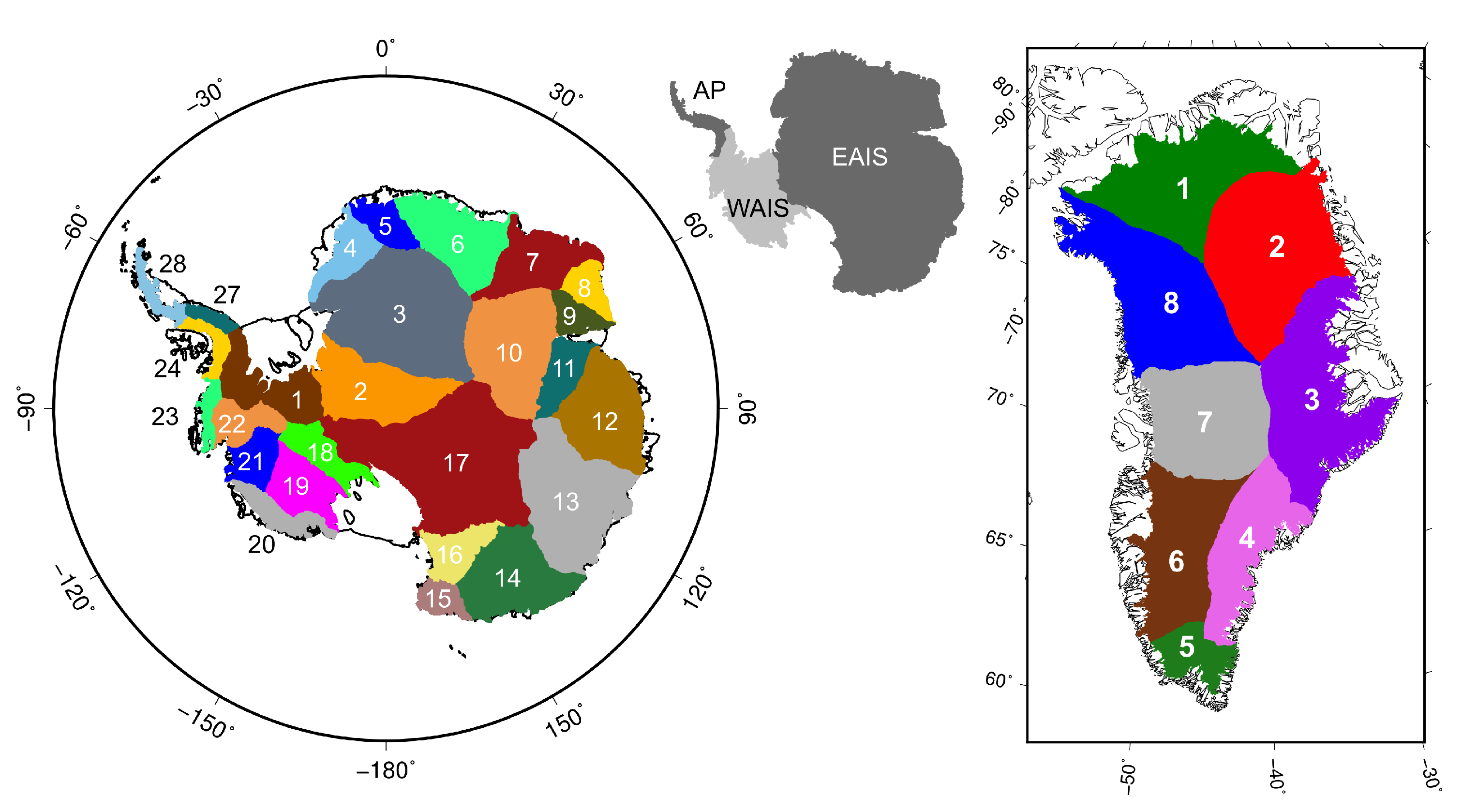
Mass change time series per basin needed to be inferred for individual drainage basins of both ice sheets as well as for several basin aggregations (Figure 1). The basins were defined according to Zwally et al. [39]. In addition to these basins, the following basin aggregations were taken into account: Antarctic Peninsula (AP), East Antarctica (EAIS), West Antarctica (WAIS), the entire Antarctica Ice Sheet (AIS) as well as the entire Greenland Ice Sheet (GIS).

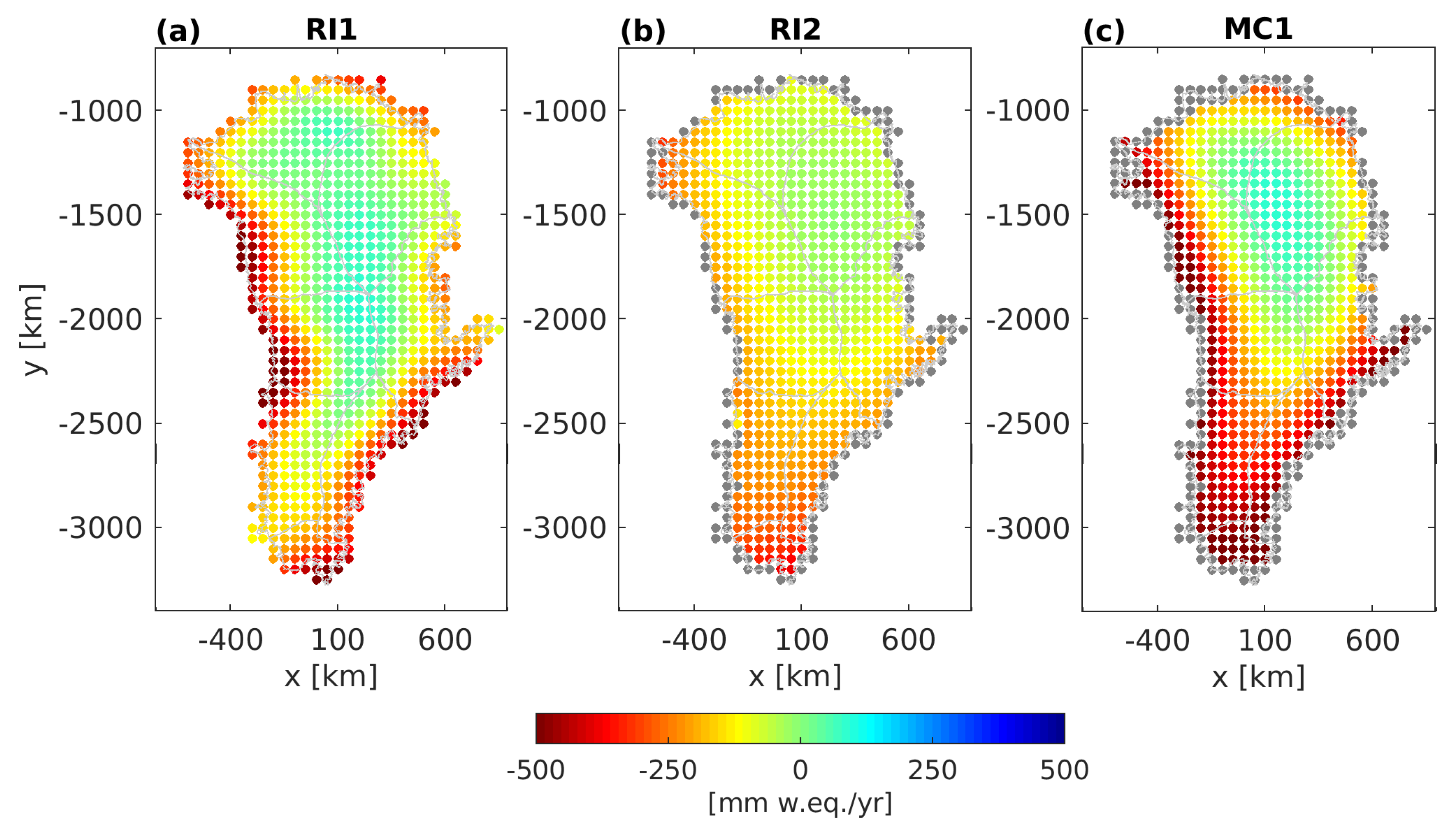
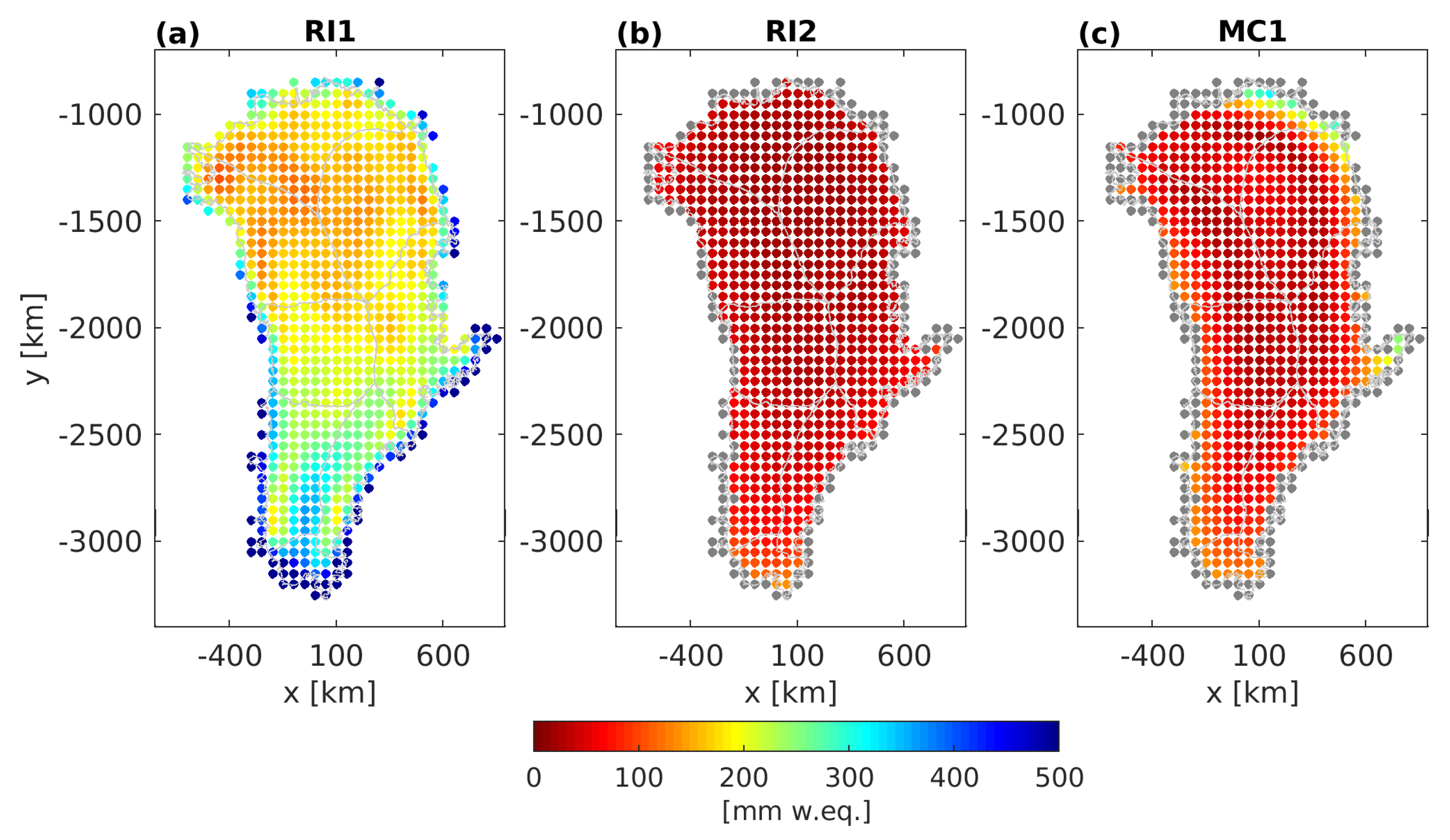
The gridded GMB product consists of one mass-change grid per epoch solely covering the ice sheet. These grids are defined in a polar-stereographic projection with a formal spatial resolution of 50 km × 50 km. Hence, gridded results had to be provided using the same grid domain and projection. Since the gridded results were only evaluated over the ice sheets, a well-performing algorithm needs to effectively restore leaked-out signal back to the ice sheet.

Mass changes per basin and mass-change grids also had to be derived from the 27 individual synthetic data sets. Therefore, each synthetic data set had to be treated in the same way as the series of GRACE monthly solutions. Of course, replacing C${}_{2,0}$, adding degree one coefficients and applying corrections for GIA was not necessary when processing the synthetic data.

2.4. Assessment of Results

Ideally, an appropriate algorithm for the generation of GRACE-derived mass change products needs to minimise both GRACE error effects (i.e., the noise) and leakage errors. To validate how this trade-off was realised by the different approaches applied in the exercise, the assessment comprises the following steps:

(A)

Visual inspection of the mass change time series

(B)

Comparison with independent data sets (if possible)

(C)

Quantification of the temporal changes

(D)

Quantification of the noise level

(E)

Comparison of the synthetic results and the underlying synthetic truth

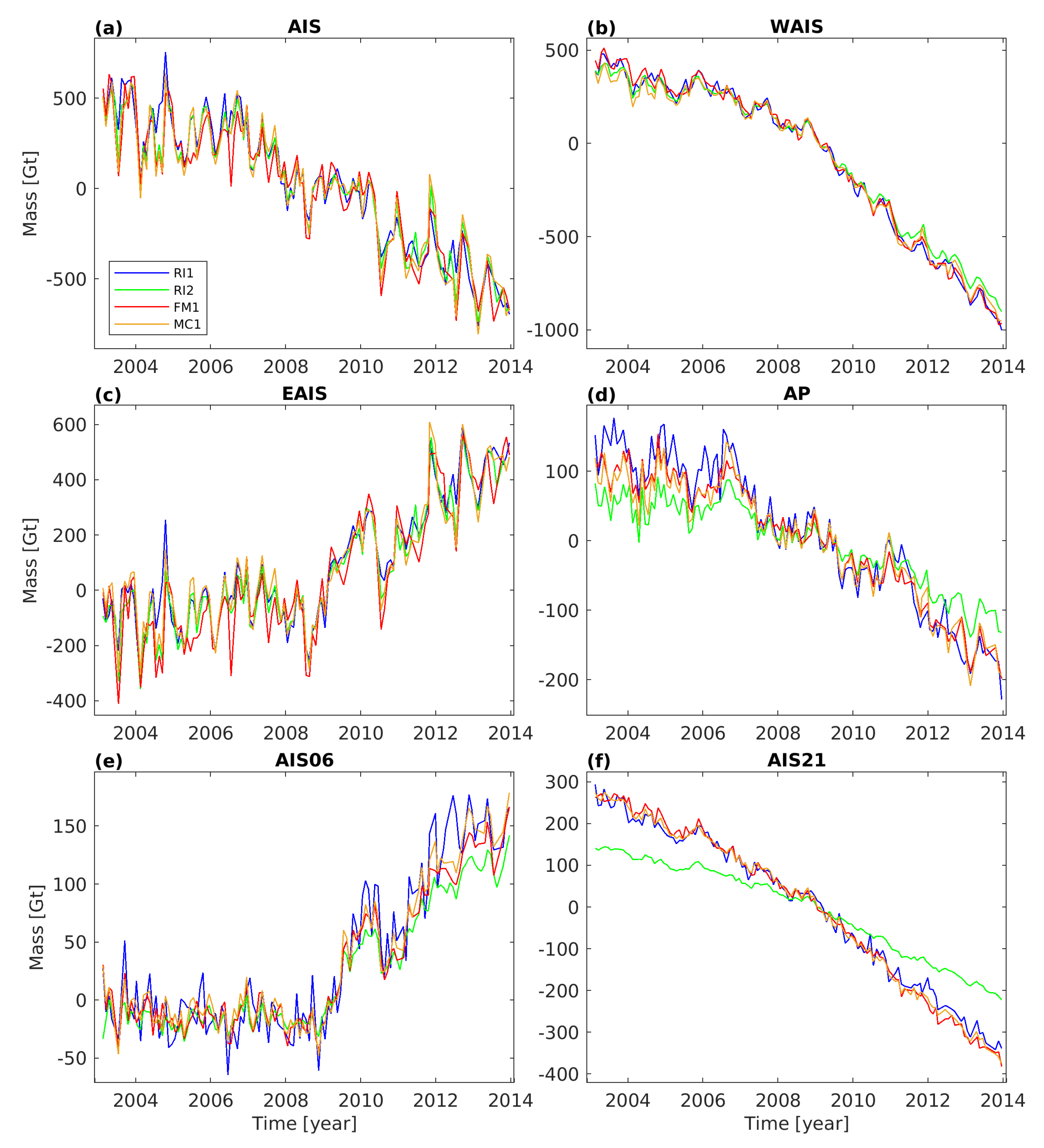
(A) Visual inspection of the mass change time series

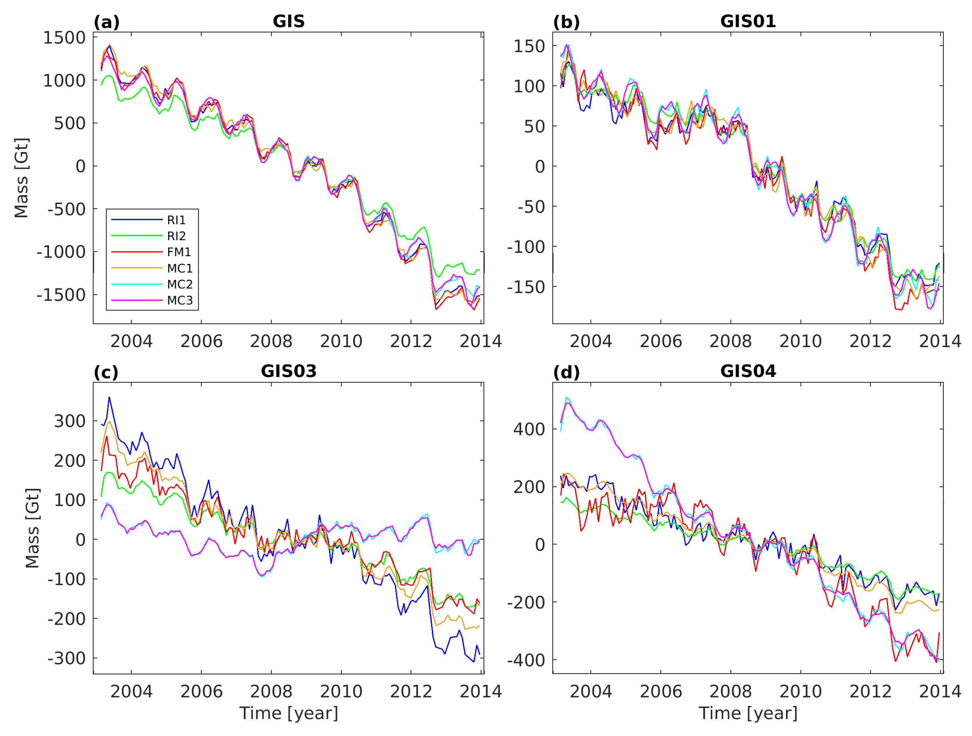
A visual inter-comparison of the different results was used to get a first impression of the level of agreement. Obvious difference both in signal content and noise level could be identified. The quantification of the revealed differences took place in the subsequent steps of the assessment.

(B) Comparison with independent data sets

An ideal validation data set consists of an independent observation of changes in ice mass, carried out by an alternative sensor. This sensor needs to be more precise and provide an identical spatial coverage at higher spatial resolution. Hence, a data set with a temporal resolution of one month and a spatial resolution better than 50 km, covering the entire AIS, is be required. However, no sensor except of GRACE is able to directly observe changes in mass with a comparable or even better spatial and temporal coverage. Therefore, observations of alternative quantities related to mass changes have to be used after applying an appropriate conversion. For example, changes in the ice sheet’s surface elevation can be converted into mass changes using an assumption of the density. A comprehensive overview of different approaches suitable for determining ice mass changes is given by Shepherd et al. [18].

Only a few independent data sets, fulfilling the requirements listed above, are available. We made use of an updated elevation time series derived from several radar altimetry (RA) satellites originally compiled by Shepherd et al. [18]. As described in Section 2.2, the volume-mass-conversion was performed using a prescribed density mask which discriminates between regions where fluctuations in elevation occur with the density of snow or ice [28]. Integrated mass change time series are available for EAIS and WAIS. However, because of the limitations of RA (e.g., sampling issues along the steep coastal margins or errors in the density assumption used for the volume-mass-conversion), this independent data set cannot provide a true reference value suitable to be used in a rigorous validation.

Due to the limited number of independent data sets available, we considered a wider range of data sets for the comparison with the GRACE results derived within the exercise. We included the reconciled mass change time series for EAIS and WAIS from IMBIE-2 [19], which are a combination of results from different techniques (satellite gravimetry, satellite altimetry and input-output-method). Moreover, we also made use of alternative GRACE products. First, mass change time series for AP, EAIS, WAIS, AIS and GIS from an additional mascon approach [16] were utilised and are referred to as “Schrama” in the following. Although this approach is consistent with our exercise in the sense that it works on Level-2 GRACE data and that the treatment of degree one and C${}_{2,0}$ is identical, there is no consistency with respect to the applied GIA corrections. Second, we made use of three different mascon products, which are directly derived from GRACE Level-1 data, to generate mass change time series for all drainage basin and aggregations of both AIS and GIS. The mascon products are provided by CSR (RL05 mascons, v01 [40]), JPL (GLO.RL05M_1 v02, CRI v02 [41]) and GSFC (v02.4 [42]). Hereinafter, time series based on these products are referred to as CSR MC, JPL MC and GSFC MC, respectively. Where necessary, we replaced the GIA correction applied by the processing centres with the correction used in our inter-comparison exercise.

The comparison of the products generated within the exercise with those from independent and alternative data sets is provided and discussed in Section 4.

(C) Quantification of the temporal changes

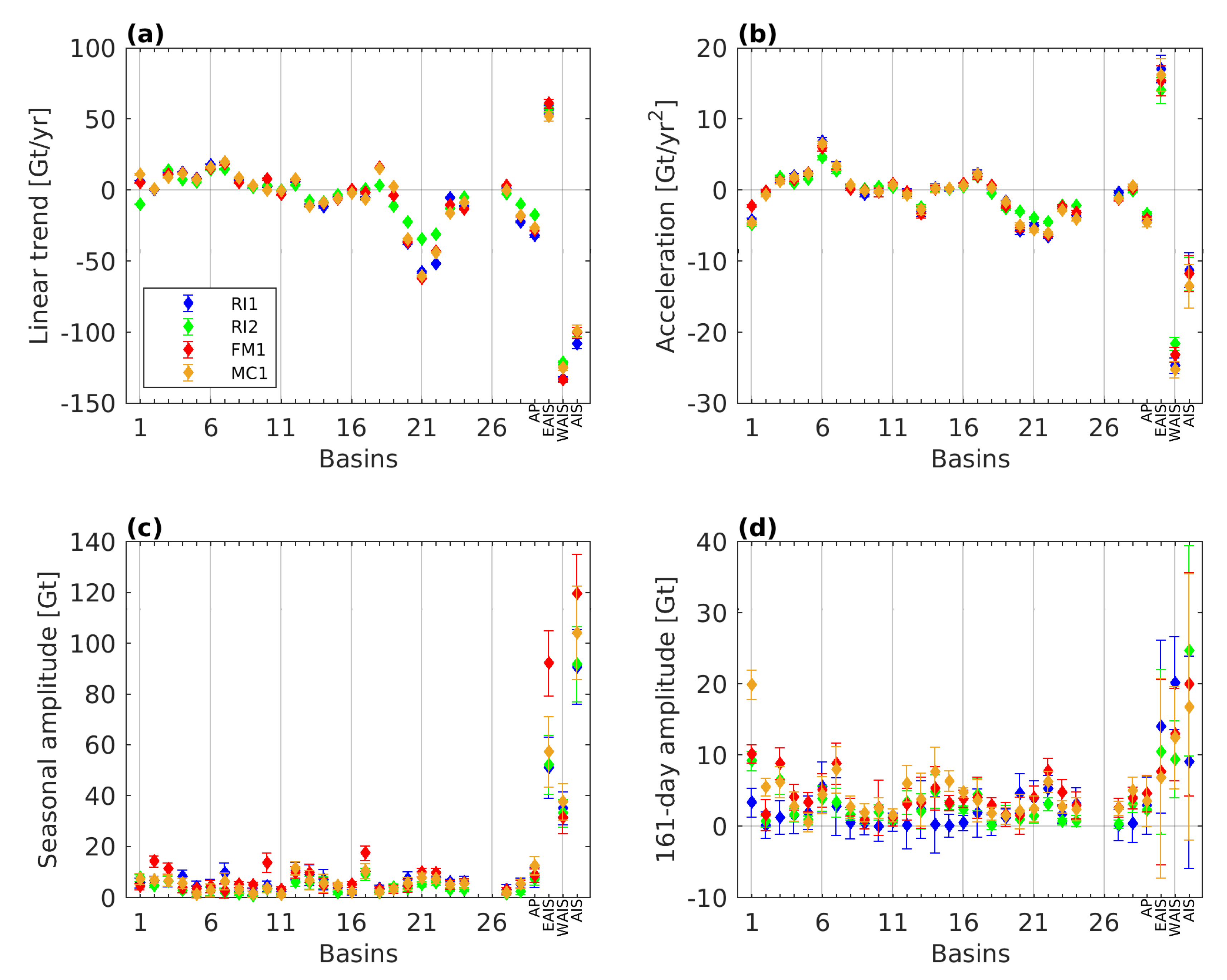
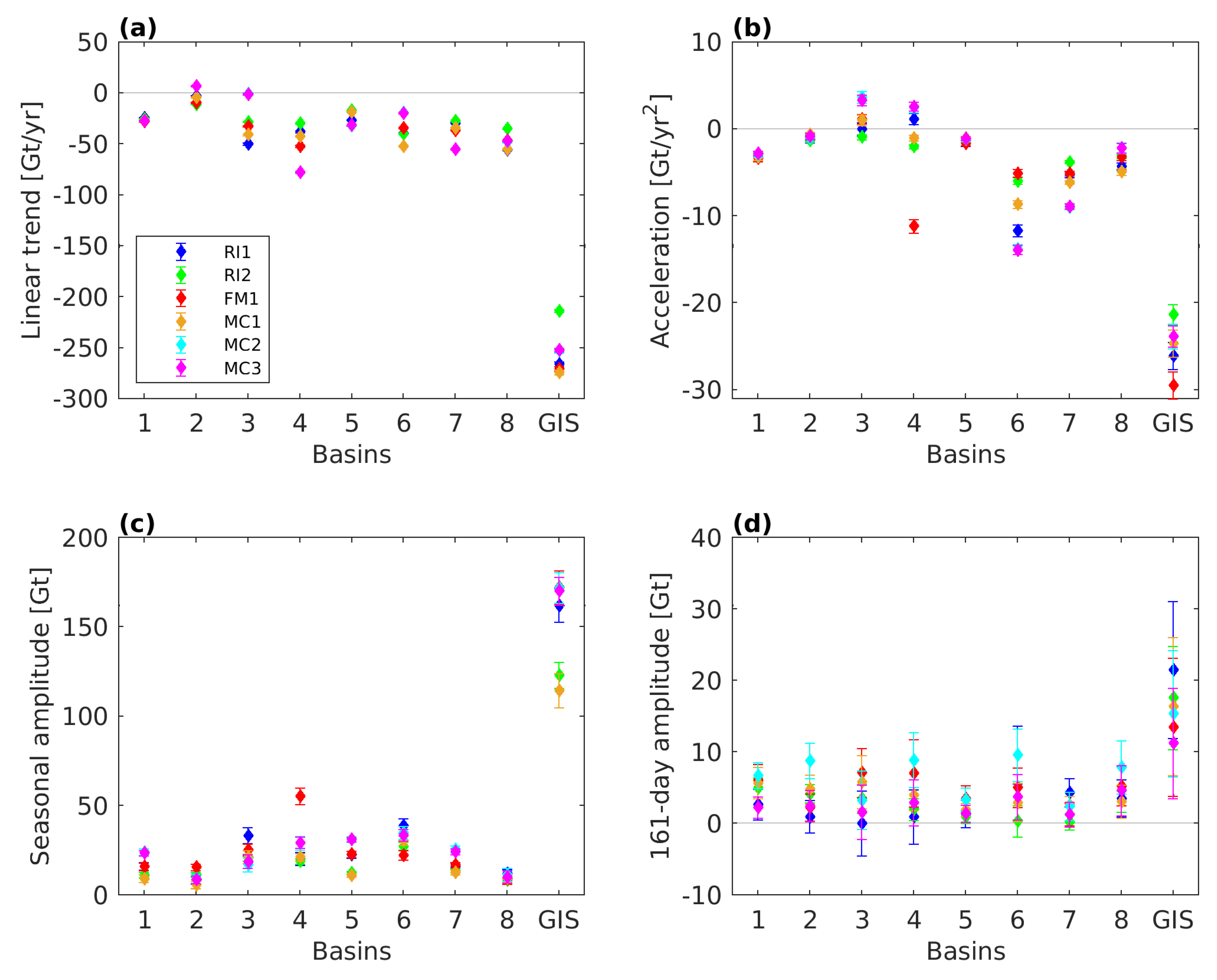
Temporal changes in mass change time series were quantified by fitting a linear, periodic (1 year, 1/2 year, 161 days) and quadratic model,

$$y\left(t\right)=a+bt+\sum _{i=1}^3\left(c_{i}sin\left(\frac{2\pi }{T_i}t\right)+d_{i}cos\left(\frac{2\pi }{T_i}t\right)\right)+e\frac{t^2}{2},T_i=1yr,1/2yr,161/365.25yr$$

(1)

with t being the time relative to the middle of the entire observational period, and by applying an equal weight to every month. Hereinafter this model is referred to as the standard model. The periodic terms account for the dominant periods of geophysical signals (annual and semi-annual) and for the 161-day alias period caused by errors in the S2 tide correction [43]. The quadratic term accounts for a possible acceleration in the mass change time series. Although alternative models are possible, this model was consistently applied to all data sets. We solved for the model parameters and derived formal errors for each parameter by means of a least squares adjustment.

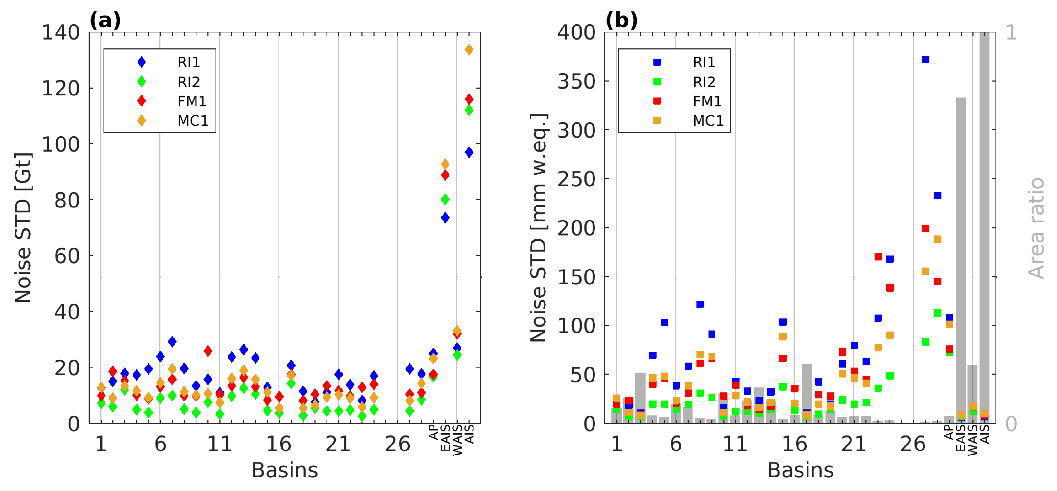
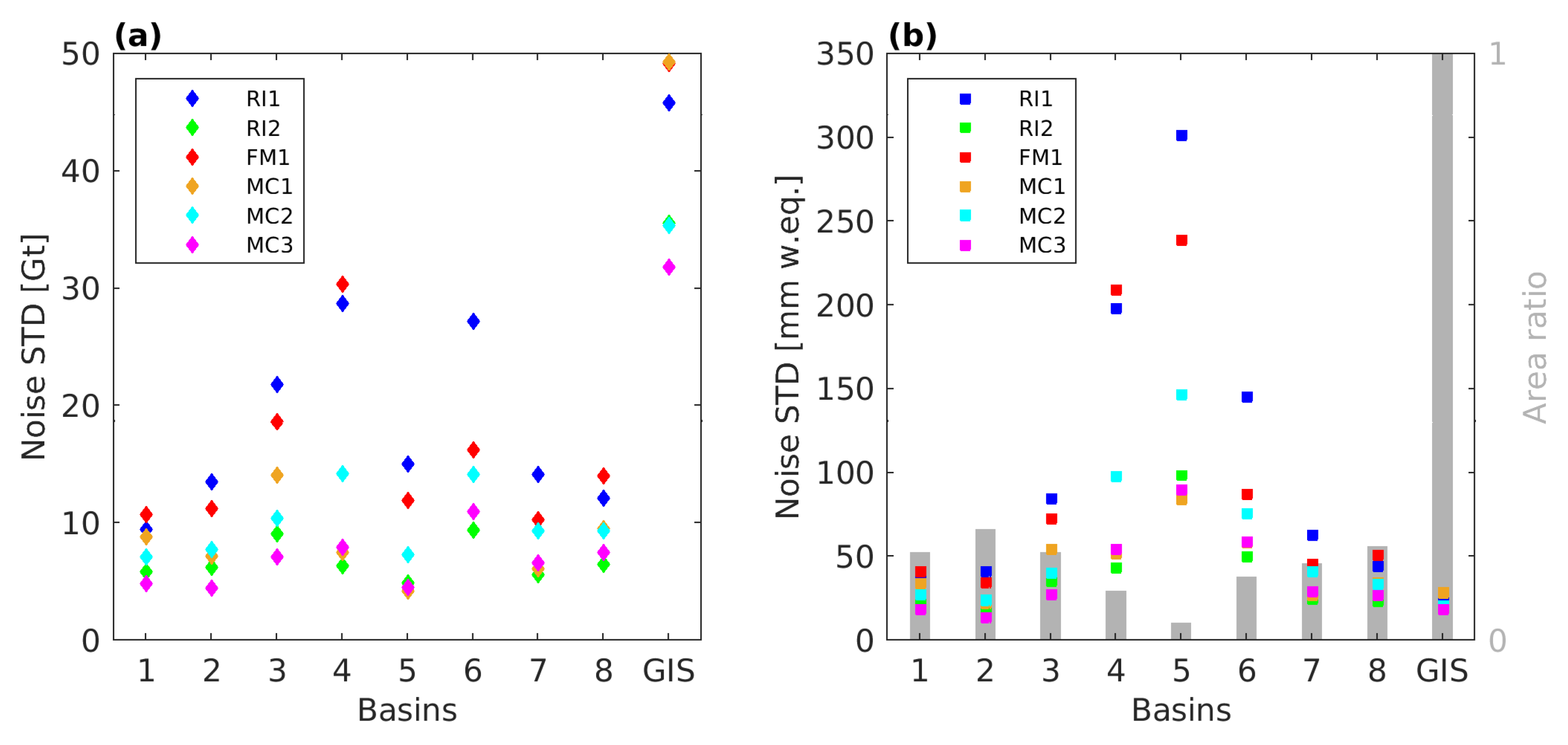
(D) Quantification of the noise level

The level of temporally uncorrelated noise in the time series was quantified. This noise includes the errors of the GRACE monthly solutions, but may also include effects of errors in the de-aliasing models, e.g., for atmospheric mass variations. In addition to a noise measure derived from the mass change time series, we also calculated a noise measure from the average surface density (i.e., mass per area) time series, which accounts for the area of the drainage basin.

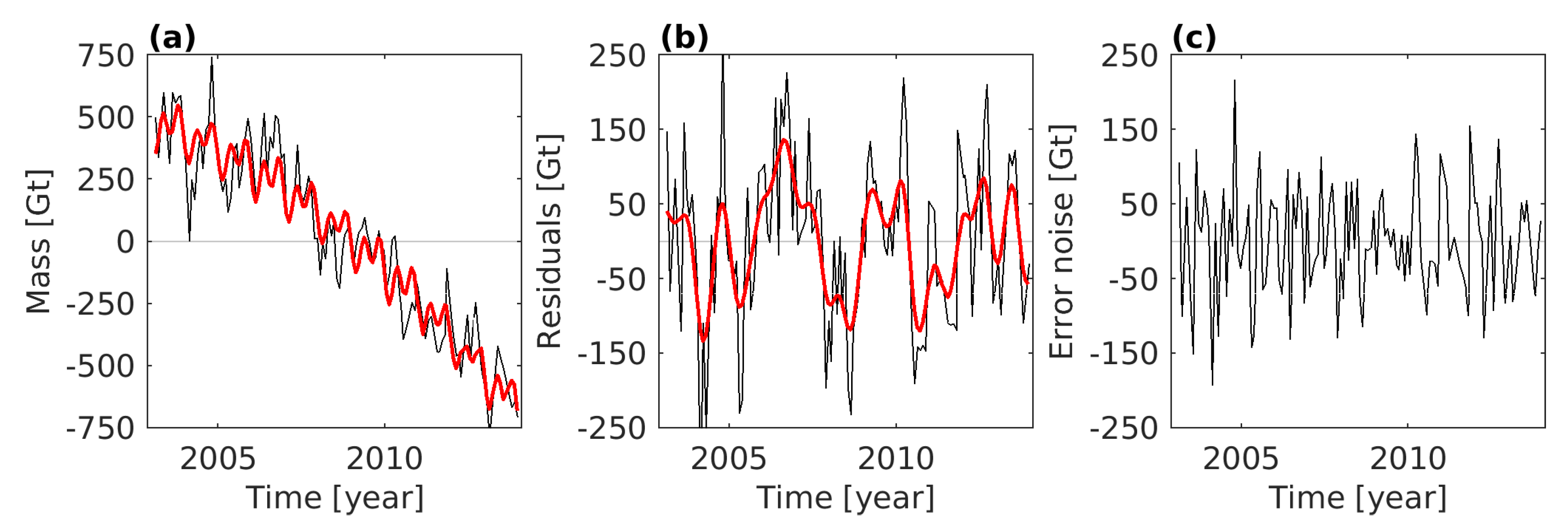
The method for quantifying the noise level is illustrated in Figure 2. First, the major long-term and periodic signal components were removed by means of the already mentioned model. Residuals of the fitted model still contain both error effects and un-modelled mass changes (e.g., inter-annual changes). To remove still present mass signals a high-pass filter based on a Gaussian average ($\sigma =2.17$ months, corresponding to a $6\sigma$ filter width of 13 months) was applied in a second step. The remaining high frequency residuals, which do not account for any low frequency components or biases, were used to assess the noise level. The calculated standard deviation was scaled to account for the fact that part of the temporally uncorrelated noise content was dampened by the preceding steps of model reduction and high-pass filtering. The scaling factor (1.35) was derived through simulations with random noise time series. Hereinafter, we refer to the scaled standard deviation of the noise time series as the noise level. The applied approach may overestimate the actual noise level, since the residuals may still contain signal. On the other hand, the method ignores possible temporal correlations of the errors in monthly GRACE solutions.

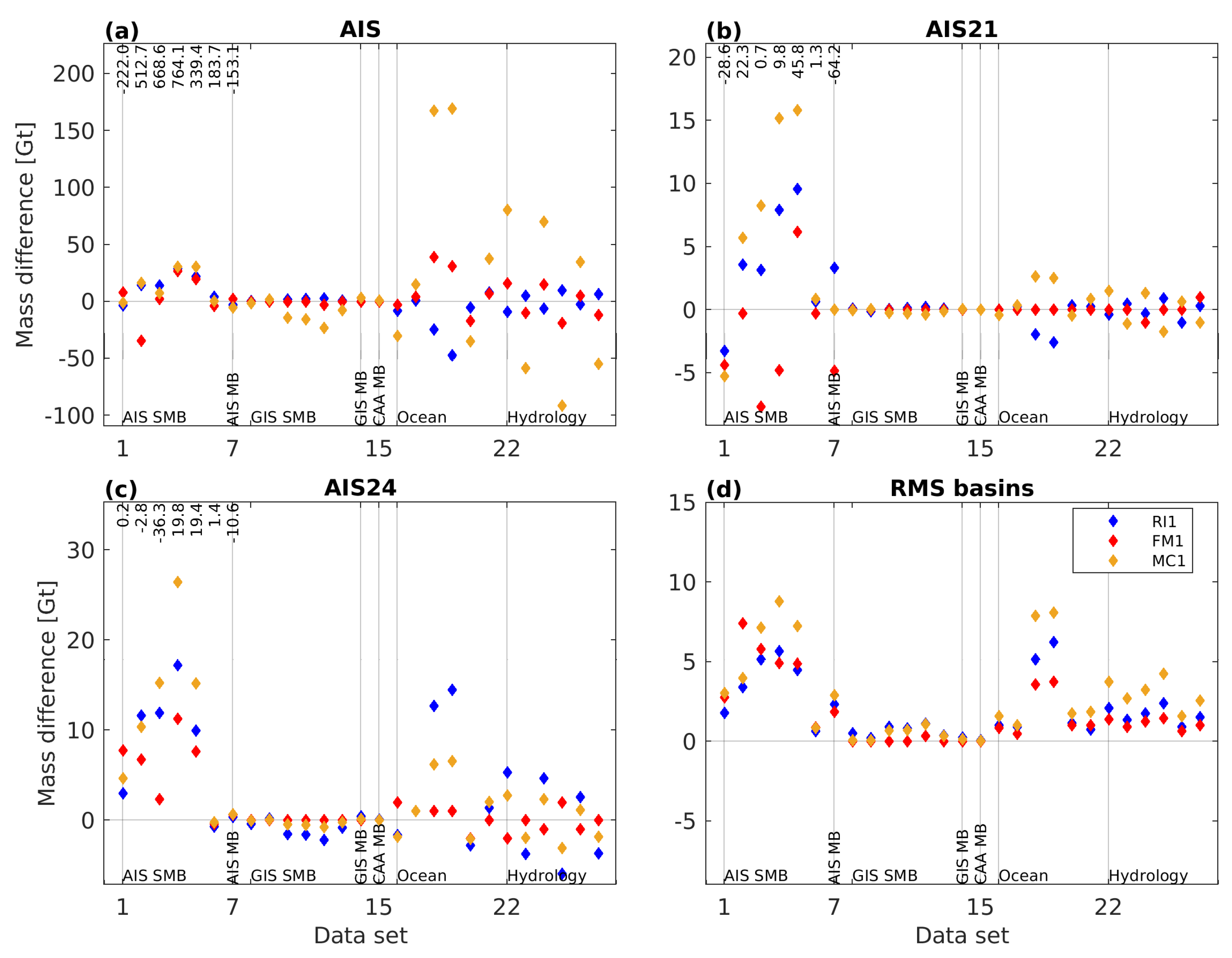
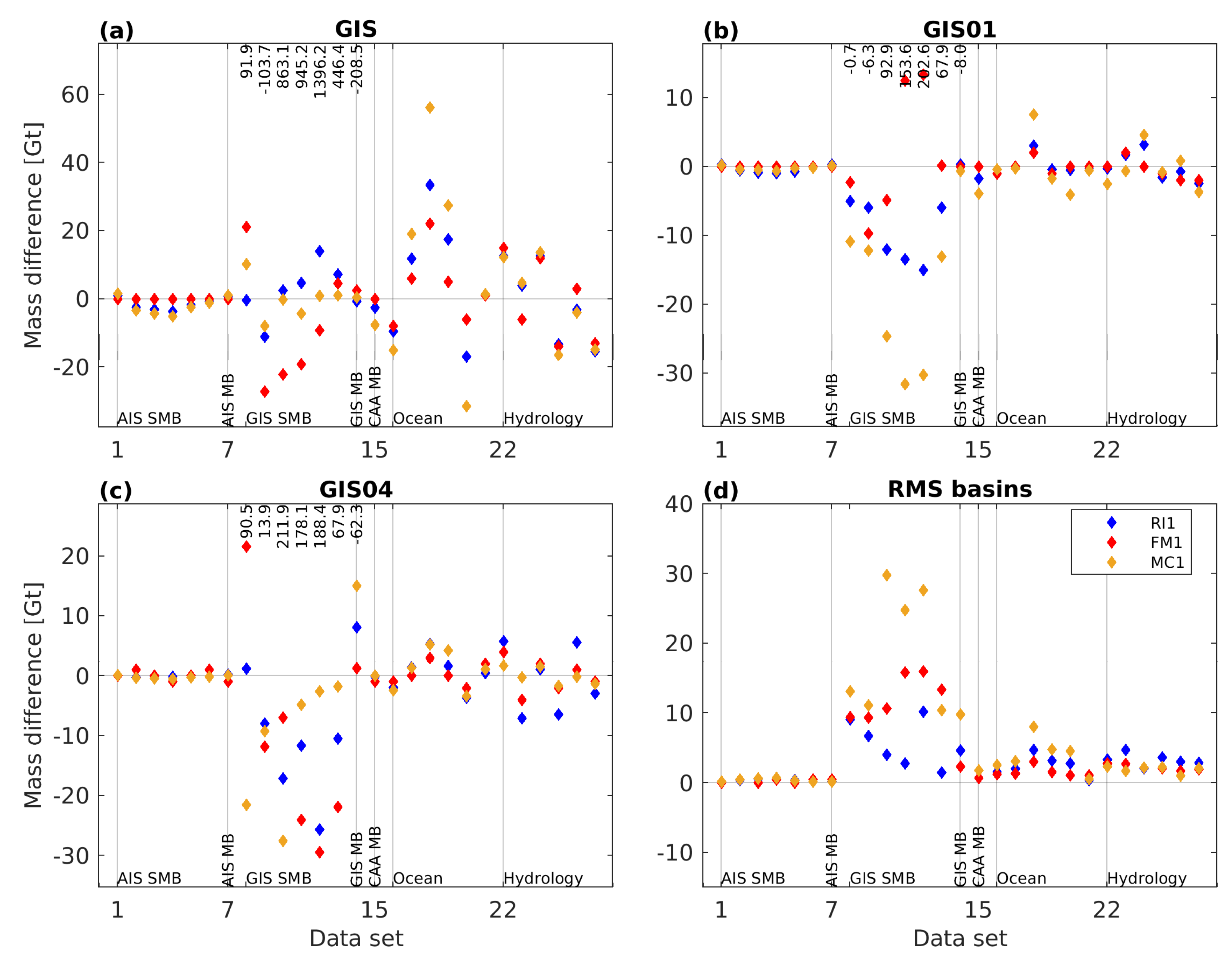
(E) Comparison of the synthetic results and the underlying synthetic truth

Mass change estimates for ice sheet drainage basins and aggregations derived by processing the spherical harmonic coefficients of the 27 synthetic data sets (Table 1) were compared to the true mass changes (synthetic truth) of the underlying original data set. The differences are used as measures for the leakage errors of the basin under investigation, induced by the signal which is mimicked by the corresponding synthetic data set. For all data sets mimicking mass changes outside the ice sheets, i.e., data sets 08–27 in case of the AIS and data sets 01–07,15–27 in case of the GIS, the synthetic truth is zero by definition for any ice sheet basin. The true mass change of all synthetic data sets covering the studied ice sheet basin or aggregation, i.e., data sets 01–07 in case of the AIS and data sets 08–14 in case of the GIS, is derived by integrating the original high-resolution gridded input data as described in Section 2.2.

It was intended to perform this inter-comparison for both the basin-averaged and the gridded results. Because of the limited number of gridded results from the synthetic data sets submitted by the participants, the assessment was limited to the synthetic results per drainage basin (Section 3.1).

3. Results

The subsequent subsections present and discuss both basin averaged and gridded results for AIS and GIS separately and follow the assessment outlined in Section 2.4. In addition to the selected results presented hereinafter, a compilation of the results for all drainage basins and aggregations can be found in the supplementary material.

3.1. Submissions

After 13 individuals had registered at the exercise website and downloaded the instructions and data sets, five different groups finally participated in the exercise. The results were provided by research groups at University of Bristol, TU Delft, DTU Space Copenhagen, TU Dresden and Ohio State University. Each contribution is referenced throughout this document using an ID based on the utilised processing approach. All approaches make use of Level-2 spherical harmonic solutions. Three different methods were applied in different variants, namely, regional integration approaches (RI), a forward modelling technique (FM) and different mass concentration (or mascon) methods (MC). The term “mascon” is manifold and can also be applied to the forward modelling method. However, here we followed the notation of the contributing group and denoted the approach as “forward modelling”.

RI1 [44] results were inferred by a regional integration approach in the spherical harmonic domain using tailored sensitivity kernels. For every basin or even grid cell a kernel was designed using different constraints (optimised by means of synthetic data sets) which allow to control signal leakage and the impact of GRACE errors using empirical error variance-covariance information. RI2 [45,46] used a regional integration approach in the spatial domain based on gridded equivalent water heights. A leakage correction was used to restore mass leaked to the ocean back to the ice sheet. The forward modelling approach FM1 [15] prescribes ice mass changes that are uniform within the coastal and the inland part of each basin. In an iterative procedure, the set of prescribed uniform mass changes was adjusted in order to fit the GRACE-observed changes in equivalent water height until convergence is reached. MC1 [17] made use of a point mass inversion scheme. GRACE-observed gravity disturbances at satellite altitude are related to point masses evenly distributed on an icosahedron-based grid. A comparable approach was used by MC2 [47,48], where gravity disturbances at satellite altitude were converted into mass anomalies in the drainage basins. A unique feature of the MC2 approach is data weighting based on the full error variance-covariance information for each monthly solution. This group has provided a second, regularised solution based on the MC2 results. The regularisation considers temporal correlation within the mass change time series. This solution is referred to as MC3 [49]. An overview of submissions from each approach is given in

Table 2. Spatial coverage of the results contributed by five groups, derived from GRACE data and synthetic input data. Basin-scale products comprise all prescribed basins and the entire ice sheet (Figure 1).

ID	RI1	RI2	FM1	MC1	MC2/MC3
Results from GRACE data
Basin mass changes	AIS, GIS	AIS, GIS	AIS, GIS	AIS, GIS	GIS
Grids	AIS, GIS	AIS, GIS	None	AIS, GIS	None
Results from synthetic input data
Basin mass changes	AIS, GIS	None	AIS, GIS	AIS, GIS	None
Grids	AIS, GIS	None	None	None	None

.

All groups have submitted GRACE-derived mass change time series per basin for the GIS, while all except one group have submitted basin-averaged GRACE results for the AIS. Three out of five participants provided time series of GRACE-derived gridded mass changes (both for AIS and GIS). The same applies for the basin-averaged results from synthetic data sets. RI1, FM1 and MC1 have provided these results for both AIS and GIS. Gridded results from synthetic data were submitted by a single group (RI1). The absence of synthetic results severely limits the possibilities to thoroughly assess the retrieval of ice mass signals by the different algorithms.

Not all participating groups were able to adjust their algorithms and processing chains to fulfil the full range of assigned tasks (e.g., processing of synthetic data) and to follow the prescribed product specifications (e.g., use the consistent grid definitions) as described in Section 2.3. Consequently, the largest number of results were submitted for the most common type of products used in ice mass studies: basin mass change time series. The number of results for the gridded products and from the synthetic data sets was clearly smaller. Considering the number of participants and the completeness of the individual submission, it becomes clear that our inter-comparison exercise does not fully meet the strict definition of a Round Robin Experiment.

A summary on the utilised data sets and applied methods is given in

Table 3. Selected details on the data sets and the processing strategy used by each participating group.

ID	RI1	RI2	FM1	MC1	MC2/MC3
Software specifications
Software	Matlab code	C code	Fortran code	Fortran code	Fortran code, Matlab code, UNIX scripts
Data used
GRACE data	CSR RL05 [20]	CSR RL05 [20]	CSR RL05 [20]	CSR RL05 [20]	CSR RL05 [20]
Period	2003-02– 2013-12	2003-01– 2013-12	2003-01– 2013-12	2003-01– 2013-12	2003-01– 2013-12
$l_{\max }$	96 (used: 90)	60	60	60	96
Degree 1	[22]	[22]	[22]	[22]	[22]
C${}_{2,0}$	[21]	[21]	[21]	[21]	[21]
GIA	[23,25]	[23,25]	[23,25]	[23,25]	[23,25]
Methods applied
Methods for mass changes per basin	Regional integration with tailored integration kernels [44]	Regional integration  [45,46]	Forward modelling [15]	Mascon [17]	Mascon [47,48,49]
Filtering	Empirical GRACE error variance and covariance model	300 km Gaussian	150 km/250 km Gaussian	DDK [8]	None

. Since RI1 decided to exclude the monthly solution 2003-01 from their time series, all subsequent analysis steps were performed for the period common to all submissions, i.e., the period from 2003-02 to 2013-12.

3.2. The Antarctic Ice Sheet

3.2.1. GRACE-Derived Mass Changes per Basin

(A) Visual inspection of the mass change time series

Figure 3 compares the different mass change time series for AIS, EAIS, WAIS and AP. In addition, time series for single drainage basins in Dronning Maud Land (AIS06) and the Amundsen Sea Sector (AIS21) are shown. All remaining basins are illustrated in Figures S1–S5. Please note the different scales among the panels. Differences in the temporal evolution as well as in the noise level are clearly visible. For some basins, time series provided by RI2 exhibit deviating temporal changes compared to the other solutions. This applies both to regions experiencing an increase and decrease in ice mass. Basin AIS06 experienced a mass gain caused by two exceptional large accumulation events in 2009 and 2011 [50]. The dynamic mass loss of basin AIS21 observed by RI2 is significantly smaller compared to the other solutions.

(C) Quantification of the temporal changes

Figure 4 illustrates the temporal variations in mass change time series derived using the standard model, i.e., linear trend, acceleration, amplitudes of seasonal (combined annual and semi-annual) and 161-day signal. The numerical values of all estimated parameters including their formal errors from the least squares adjustment are summarised in Tables S1–S3.

The linear trend estimates and their formal errors are shown in Figure 4a. For the entire AIS, trend estimates from the participants’ time series vary between −99 Gt/yr and −108 Gt/yr. Larger discrepancies can be found at basin scale. The corresponding formal errors cover the range between ±3 Gt/yr and ±4 Gt/yr, and are even smaller for most of the basins and therefore hard to identify in the plot. For the majority of basins revealing significant loss in ice mass (e.g., in West Antarctica), the loss rates for RI2 are clearly the lowest. At the same time, RI2 observes the lowest mass gain for basins in East Antarctica. However, since all participants made use of the same GRACE monthly solutions, background models and corrections, the revealed discrepancies are solely due to different methodologies.

Various studies (e.g., [10,51]) have shown that the consideration of deviating input data may even lead to larger discrepancies. For the AIS and the period 2005–2015, Blazquez et al. [51] found that trends from GRACE solution series provided by the three official processing centres differ up to 4 Gt/yr, although the differences can be about one order of magnitude larger for other processing centres. We found that the impact of the maximum spherical harmonic degree $l_{\max }$ does not exceed 5 Gt/yr, when considering $l_{\max }$ = 90 and $l_{\max }$ = 60 in the method applied by RI1 (Figure S6). On the other hand, trend differences induced by the utilisation of deviating time series for degree one and $C_{2,0}$ coefficients can be as large as 29 Gt/yr and 7 Gt/yr, respectively [51]. It is noteworthy, that the spread induced by different degree one time series is larger than the total effect caused by the degree one time series used by the participants. For example, for method RI2, the neglection of degree one would reduce the AIS mass loss by 19 Gt/yr (Figure S6). By far the largest error in GRACE-based mass balance estimates is caused by uncertainties in recent GIA models [11]. Trends from various models differ by up to 61 Gt/yr [51].

Figure 4b depicts the co-estimated acceleration terms for all basins and aggregations. The AIS estimates range from −11 Gt/yr${}^2$ through −13 Gt/yr${}^2$ and agree within the range of the corresponding formal errors. The largest positive accelerations (among all basins and aggregations) are evident for EAIS, mainly caused by the already mentioned accumulation events, while an accelerated mass loss is clearly visible in West Antarctica (WAIS). The revealed differences between the linear trends for RI2 and the other groups also apply for the inferred accelerations.

The seasonal amplitudes are shown in Figure 4c. While the estimates for different submissions agree within the range of the formal errors for most of the basins, the seasonal amplitudes for FM1 are clearly larger for certain basins (e.g., AIS09, AIS17, EAIS). Seasonal amplitudes for AIS cover the range between 91 Gt and 120 Gt, while formal errors vary between ±15 Gt and ±18 Gt. Figure 4d depicts the amplitudes of the 161-day aliasing period, which are at the same order of magnitude as the seasonal amplitude for most of the single drainage basins. However, for larger aggregations (e.g., EAIS, WAIS, AIS), the 161-day amplitudes are considerably smaller, while their error estimates exceed the amplitudes themselves.

(D) Quantification of the noise level

Finally, the noise level of each mass change time series was evaluated as described in Section 2.4 (D). The noise standard deviation of the mass change time series for a single drainage basin is on the level between 3 Gt and 29 Gt and increases for larger basin aggregations (Figure 5a, Tables S1–S3). The noise level derived from the time series of the average surface density (Figure 5b) clearly indicates that basins of small size (e.g., AIS08, AIS24 or AIS27) are most affected by noise. Time series provided by RI2 exhibit the lowest overall noise level.

3.2.2. Synthetic Results per Basin

(E) Comparison of the synthetic results and the underlying synthetic truth

Figure 6 illustrates the differences between the results from the synthetic data sets and the true synthetic mass changes, which are measures for the leakage errors, for the entire AIS, basin AIS21 and basin AIS24. Results for all basins are shown in Figures S8–S12. For all data sets with a non-zero true mass change, i.e., data sets covering the AIS, the value of the true mass change is indicated at the top margin.

For the entire AIS the largest leakage errors are induced by residual oceanic mass changes, followed by variations in Antarctic SMB and continental hydrology. Far-field effect stemming from the GIS and CAA are negligible. It should be kept in mind that the maximum leakage is caused for two data sets where the residual oceanic mass changes are exceptionally large (Section 2.2). The size of the leakage error depends on both the magnitude and the spatial pattern of the underlying signal. For example, for the entire AIS, leakage from AIS SMB is larger than from the AIS annual mass balance pattern (AIS MB), since overall magnitude of the AIS SMB data sets is larger than for the AIS MB data set, as indicated by the synthetic truths given in Figure 6.

We chose basin AIS21 (Amundsen Sea Sector) as an example since it is dominated by dynamic thinning and therefore allows us to assess the recovery of the mean annual mass change mimicked by data set 7 (AIS MB). Figure 6 depicts that the algorithms underlying both RI1 and FM1 are able to recover the mean annual mass change equally well. While RI1 slightly underestimates the true mass loss, FM1 provides a slight overestimation. The differences are 3.3 Gt and −4.8 Gt corresponding to a relative error of about 5% and 7%, respectively. MC1 almost perfectly recovers the true mass change, with the difference being smaller than one tenth of a gigaton, only. The spread between all three leakage errors for the mean annual mass change is 8.1 Gt. This is still clearly lower than the additional error effects on the linear trend described in Section 3.2.1 (C). For comparison, the spread between the three linear trend estimates derived from the GRACE time series for AIS21 is 3.8 Gt/yr (RI1 being less negative than MC1 and FM1). We also found that the different maximum spherical harmonic degree used by the participants has a minor impact on the corresponding leakage errors (Figure S20).

Basin AIS24 (George VI Sound) is located close to Alexander Island whose changes in surface mass balance are included in the synthetic data sets 1–6 (AIS SMB). Therefore, the algorithm’s ability to separate these nearby signals can be studied. Like for other basins, the largest leakage errors are induced by SMB variability. However, for basin AIS24 the SMB-induced leakage is clearly larger compared to other basins. For example, in comparison to basin AIS21 the leakage error may be about twice as large, depending on the magnitude of the SMB signal. For most of the synthetic data sets on SMB variability, FM1 results exhibit the smallest leakage errors for basin AIS24.

For a more comprehensive assessment, we need to consider all drainage basins. Leakage errors depend on the magnitude and pattern of the inducing signal, the area of the basin under investigation or, in case of leakage caused by the nearby ocean, on the length of the shoreline. Hence, leakage errors differ between the basins. Figure 6d gives a general overview on the leakage errors showing the root mean square (RMS) of the differences between the individual synthetic estimates and the synthetic truth for all drainage basins constituting the entire AIS. It becomes evident that leakage induced by AIS SMB variability is largest, while far-field changes in ice mass (GIS and Canadian Arctic) are negligible. Leakage caused by errors in the oceanic component of the GRACE de-aliasing product may be in the same order of magnitude as errors caused by continental hydrology. Hence, basin-averaged monthly mass change estimates derived from GRACE may exhibit leakage errors in the order of 10 Gt, on average. The large errors for oceanic data sets 18 and 19 are related to gross errors in the de-aliasing product and can be considered an upper limit. In general, no coherent differences could be identified in the overall performance of RI1 and FM1 for the dominant leakage signals (AIS SMB and Ocean), although RI1 performs slightly better in terms of AIS SMB signal leakage, whereas FM1 performs best in terms of the Ocean signal leakage. MC1 exhibits slightly larger leakage errors stemming from signals in the ocean and continental hydrology.

3.2.3. GRACE-Derived Gridded Mass Changes

The gridded results submitted by the different groups differ with respect to their representation (e.g., regular geographic grid projected to a polar-stereographic plane, regular polar-stereographic grid or an icosahedron grid). For the AIS, three sets of gridded results are available, namely, RI1, RI2 and MC1. These data were used to quantify temporal changes and the noise level for each grid cell as described in Section 2.4 (C) and (D), respectively. However, this did not allow us to directly compare the results from different groups. For a quantitative comparison, all but the RI1 results for the linear trend and the noise level were interpolated to the prescribed polar-stereographic grid with a grid spacing of 50 km× 50 km grid (Section 2.3). In this step we did not extrapolate beyond the domain of the original grids. Hence, all cells of the polar-stereographic grid lying outside the original grid domain were ignored in the comparison.

(C) Quantification of the temporal changes

Figure 7 reveals significant differences between the patterns of the linear trend. Since the linear trends for the entire AIS are nearly identical for MC1 and RI2 (Figure 4), the same applies for the averages of the gridded trends (−8.3 and −8.1 mm w.eq./yr). The small difference arises from differing areas covered by the interpolated gridded products. In theory, if two algorithms are comparably effective in restoring ice mass changes back to the ice sheet, a smaller solution area would result in a larger change in surface density, both in terms of the average as well as the extreme values. However, existing differences in the extreme values visible in Figure 7 indicate differences in the algorithms’ performance. Both the mass loss in West Antarctica and the mass gain, e.g., along coastal regions of East Antarctica (Dronning Maud Land), are clearly the weakest for RI2. While the trend for MC1 ranges from −678.7 to 208.3 mm w.eq./yr, the trend for RI2 varies between −284.3 and 53.8 mm w.eq./yr, only. The largest average mass loss trend is revealed for RI1 (−8.5 mm w.eq./yr), even though their extreme values (−562.2 and 185.6 mm w.eq./yr) do not exceed those of MC1. Moreover, RI1 exhibits features of smaller scale in terms of more localised mass trend patterns (e.g., over the Kamb Ice Stream). The largest differences are revealed between MC1 and RI2, with an RMS of 49.0 mm w.eq./yr, while the RMS of the differences between MC1 and RI1 is 36.8 mm w.eq./yr, only. The RMS difference between RI1 and RI2 is 41.7 mm w.eq./yr.

(D) Quantification of the noise level

Figure 8 reveals large differences between the noise levels of the gridded products. The largest noise level was found for RI1 with an RMS of 229.7 mm w.eq. In particular, coastal regions are heavily affected by noise, exceeding the 500 mm. w.eq. level. Over the ice sheet artefacts of GRACE striping patterns are still visible. The noise level of MC1 (RMS: 92.5 mm w.eq.) is clearly lower than for RI1. However, larger noise along the coastal margins, compared to the interior of the ice sheet, can also be observed for MC1. By far the lowest overall noise level is revealed for RI2, which shows only minor variations over the AIS, with slightly increased value at the tip of the Antarctic Peninsula (AP). The RMS for RI2 (32.8 mm w.eq.) is about one order of magnitude smaller than for RI1. Hence, the largest differences are found between the noise levels of RI1 and RI2. The RMS of the differences calculated for all common grid cells is 169 mm w.eq.

Synthetic data sets can help to identify the origin of the larger noise in coastal regions. Figure 6 reveals the largest leakage errors for the data sets mimicking residual oceanic mass changes (Table 1). However, these basin-integrated estimates do not allow for an assessment of the spatial patterns. This information can only be derived from gridded results derived from the synthetic data sets, which were solely provided by RI1 (Table 2). We found that gridded leakage errors derived from synthetic data sets 16–21 (not shown) can be as large as 500 mm w.eq. along the coastline. The same also applies to other synthetic data mimicking far-field signals, e.g., from the continental hydrology (data sets 22–27), which also include an oceanic component through the mass conserving ocean layer.

3.3. The Greenland Ice Sheet

3.3.1. GRACE-Derived Mass Changes per Basin

(A) Visual inspection of the mass change time series

Mass change time series for the entire GIS as well as basins GIS01 (northern GIS), GIS03 (eastern) and GIS04 (south-eastern) are compared in Figure 9. Figures for all GIS basins are provided in the Supplementary Materials (Figures S14 and S15). Note that MC2 has provided an additional, regularised solution referred to as MC3. The most northern basin GIS01 is closest to the Canadian Arctic Archipelago and potentially affected by leakage-in. Differences in the temporal evolution and the noise content are evident for every basin. Time series provided by RI2 reveal the smallest loss in mass for the entire GIS. For basin GIS03 the MC2/MC3 time series clearly deviate from the majority of time series. While the decrease in ice mass is smaller for basin GIS03 the opposite is true for the neighbouring basin GIS04. This is a clear indication for differences in signal leakage, caused by the neighbouring basins, among the various results. These differences can only be verified by means of synthetic data sets.

(C) Quantification of the temporal changes

Linear trends derived using the standard model and their corresponding error estimates are shown in Figure 10a. Using the standard model, the consistently inferred linear trends for GIS vary between −213 Gt/yr and −274 Gt/yr, while the corresponding formal errors of the trends derived from the least squares adjustment are in the range of ±1 Gt/yr. The significant spread between the results is mainly caused by the RI2 estimate. Excluding this result reduce the range to −252 Gt/yr through −274 Gt/yr. Numerical values for all basins are given in Table S4.

As already outlined in the section on the AIS results, different choices of input data may lead to discrepancies in the trends still exceeding the discrepancies revealed here. Blazquez et al. [51] quantified the following variations in linear trend depending on the input data (entire GIS, 2005–2015): GRACE monthly solution series: up to 10 Gt/yr, degree one: 7 Gt/yr, C${}_{20}$: 4 Gt/yr, GIA correction: 4 Gt/yr. We assessed the impact of the degree one time series through the example of RI2 and found the impact on the trend to be 4 Gt/yr. This estimate is in the same or of magnitude as the trend differences derived by Blazquez et al. [51]. The impact of the maximum spherical harmonic degree (RI1: $l_{\max }$ = 90 vs. $l_{\max }$ = 60) is no larger than 1 Gt/yr (Figure S16).

Figure 10b depicts the jointly estimated acceleration terms for all basins and aggregations. The GIS estimates range from −21 Gt/yr${}^2$ through −30 Gt/yr${}^2$, indicating an increased overall mass loss. This range is reduced to −24 Gt/yr${}^2$ to −30 Gt/yr${}^2$ if the RI2 results is excluded. The largest accelerations can be observed for the western basins GIS06 and GIS07, where an increased mass loss is observable from 2005 onwards.

The seasonal amplitudes shown in Figure 10c vary significantly between 114 Gt and 172 Gt for the entire GIS, while the corresponding errors are in the range from ±4 Gt to ±7 Gt. RI2 and MC1 exhibit clearly smaller amplitudes for GIS and most of the basins compared to the remaining submissions. Table S4 reveals that this offset mainly originates from the annual component of the seasonal amplitude. The smaller seasonal signals for RI2 are, in a way, consistent with the smaller mass loss rates (Figure 10a). This does not apply for MC1. Somewhat larger amplitudes for FM1 (e.g., basin GIS04) are in agreement with our findings for the AIS. The amplitudes of the 161-day aliasing period (Figure 10c) do not exceed 10 Gt for single drainage basins and agree within the corresponding error estimates among the different submissions.

(D) Quantification of the noise level

The standard deviations of the noise, assessed according to Section 2.4 (D), are shown in Figure 11a. The noise standard deviation for a single drainage basin time series varies between 4 Gt and 30 Gt, where the noise is higher for larger basin aggregations. The noise level derived from the average surface density time series is shown in Figure 11b and reveals that the small basin GIS05, located at the southern tip of Greenland, is mostly affected by noise. Using basin definitions which avoid very small basins like GIS05, e.g., the basin definitions used in IMBIE-2, may help to reduce the noise level of the corresponding mass change time series. Time series provided by RI2 and MC2/MC3 exhibit the lowest overall noise level. For the entire GIS, the linear trend estimates from these solutions are the least negative (Figure 10a).

3.3.2. Synthetic Results per Basin

(E) Comparison of the synthetic results and the underlying synthetic truth

Figure 12 compares the differences between the results from all synthetic data sets with the corresponding true mass changes for the entire GIS as well as basins GIS01 and GIS04. Results for all basins are depicted by Figures S18 and S19. For the entire GIS, the mean annual mass change is well recovered by all three approaches (RI1, FM1, MC1). The absolute differences between the synthetic truth of data set 14 (GIS MB) and the user estimates are below 1 Gt for RI1 and MC1, and are about 2 Gt for FM1, only. Hence, leakage errors in GRACE-derived mass balance estimates for the entire GIS are supposed to be clearly smaller than additional error effects on the linear trend, e.g., caused by uncertainties in auxiliary data sets and applied corrections (Section 3.3.1 (C)). For single drainage basins (e.g., GIS04), leakage errors associated with the pattern of the mean annual mass change can be larger than for the entire GIS. This is an indication that all algorithms are distributing mass signals between the basins. Synthetic results for data set 15 (CAA MB) allow us to study the impact of Canadian Arctic mass changes. The estimates for GIS01 are of particular interest due to the proximity of this region to the Canadian Arctic. For RI1 and FM1, the error in the GIS01 estimate caused by the mean annual mass change over CAA is below 2 Gt, while the error for MC1 is slightly larger (4 Gt). When integrating over the entire GIS, leakage errors caused by the trend in ice mass change over CAA are larger than for single drainage basins. This is the opposite of what we have observed for data set 14 (GIS MB). Hence, this source of leakage outside the GIS, and its corresponding mass changes over the ocean, may lead to slightly larger leakage errors in GRACE-derived ice mass trends for the GIS, than the GIS signal itself.

Figure 12d gives a general overview on the leakage errors across all drainage basins constituting the GIS. The RMS of the differences between the individual synthetic estimates and the synthetic truth depicts that the largest leakage errors are induced by GIS SMB variability. As a result, on average, leakage errors in the order of 10 to 20 Gt are to be expected in basin-scale monthly GRACE mass change estimates. The majority of all remaining sources of leakage considered in the exercise cause errors below 5 Gt. This includes mean changes in ice mass over GIS and CAA as well as oceanic leakage and far-field effects stemming from continental hydrology. Antarctic far-field signals are negligible. The overall performance of all three algorithms is comparable.

3.3.3. GRACE-Derived Gridded Mass Changes

Three sets of gridded results are available for the GIS: RI1, RI2 and MC1. Figure 13 and Figure 14 depict the spatial patterns of the linear trend and of the noise level, respectively. As described in Section 3.2.3, these grids were derived by interpolating the trend and noise estimates (Section 2.4 (C) and (D)) calculated for each grid cell of the original grids, to the prescribed polar-stereographic grid with a grid spacing of 50 km × 50 km.

(C) Quantification of the temporal changes

MC1 exhibits the largest average trend over the GIS (−150.9 mm w.eq./yr), followed by RI1 (−131.5 mm w.eq./yr). As for the integrated GIS mass change time series, the smallest average trend is revealed for RI2 (−103.4 mm w.eq./yr). The differences between the average trends arise from clearly more negative trends along the southern and western ice sheet margin for both MC1 and RI1 compared to RI2. Moreover, while MC1 and RI1 exhibit positive trends in central and northeast Greenland of more than 80 mm w.eq./yr, the gridded trend for RI2 are entirely negative, reaching from −389.0 to −13.6 mm w.eq./yr. Figure 13 reveals that the RI2 pattern is clearly the smoothest among the three. Both RI1 and MC1 exhibit the largest mass loss rates along the southeastern and the western ice sheet margin. However, most spatial details can be identified in the RI1 solution. In particular, along the western coast of Greenland different patterns coinciding with fast-flowing outlet glaciers (e.g., Jakobshavn Isbræ) become evident. For RI1, a less strong mass loss rate is revealed towards the coastal region of the southern part of basin GIS06 (Figure 1), which breaks up the strong near coastal mass loss in the northern part of GIS06 and in GIS05. Such a pattern is not visible for any other solution. However, we also see this pattern in the gridded synthetic results for data set 14 (mean annual mass change) provided by RI1 (not shown). Since such a pattern is not visible in the synthetic data set itself, it is an artefact caused by the RI1 algorithm. Over the entire GIS, the differences between RI1 and MC1 are the largest, with an RMS of 146.7 mm w.eq./yr, while the smallest difference are found between RI1 and RI2 (RMS: 97.6 mm w.eq./yr).

(D) Quantification of the noise level

Figure 14 clearly reveals the largest noise standard deviation for the RI1 gridded product, with an RMS of 278.0 mm w.eq. In contrast, the RMS of the noise standard deviation is 70.9 and 38.9 mm w.eq./yr for MC1 and RI1, respectively. Hence, the largest difference in the noise level are evident between RI1 and RI2 with an RMS of 174.6 mm w.eq./yr. This is comparable to what we found for the noise level of the basin-averaged mass change time series (Section 3.3.1 (D)). Since the noise averages out to some extent when integrating over larger regions, the differences between the gridded products are larger than between the basin products, for which the differences among the various products are in general decreasing with increasing size of the basin (Figure 11b).

In particular, coastal regions of the RI1 solution are heavily affected by noise, clearly exceeding the 500 mm w.eq. level. Comparable effects of smaller magnitude are visible along the north-eastern coast in the MC1 product. This is comparable to what we found for the AIS and discussed in Section 3.2.3 (D). The north-south-oriented pattern of larger noise at the southern tip of the GIS for RI1 coincides with the region of less pronounced mass loss visible in Figure 13.

4. Discussion and Conclusions

An algorithm suitable for the generation of GMB products, consisting of both time series of basin averaged mass changes and mass change grids, needs to fulfil conflicting requirements. On the one hand the algorithm has to minimise the effect of GRACE errors on the mass change estimate, e.g., by means of an appropriate filtering technique. On the other hand leakage errors need to be minimised, which will most likely be increased due to the applied filtering. Well-performing algorithms realise a trade-off between the minimisation of both error sources.

We described in detail the concept and realisation of an inter-comparison exercise. The standard deviation of the temporally uncorrelated variability has been used as a measure of the noise level. Synthetic data sets with an a priori known true mass change allow for the quantification of leakage errors. A comprehensive evaluation of an algorithm is only possible if both GRACE-derived GMB products and results of simulations with synthetic data sets, ideally both basin-average and per grid cell, are available. Moreover, a certain level of consistency with respect to the utilised data sets (e.g., the period under investigation or the applied GIA correction) and unified formats and conventions for the results to be submitted, are mandatory prerequisites for a successful comprehensive algorithm assessment.

The present study illustrates the spread between GMB products derived using different algorithms. Both temporal changes and the noise level of the products exhibit significant differences. In case of the ice-sheet-wide basin products, the consistently derived linear trends vary from −99 Gt/yr to −108 Gt/yr for the AIS and between −213 Gt/yr and −274 Gt/yr for the GIS. This large spread corresponds to 8% and 28% of the corresponding minimum mass loss rates, respectively. By excluding the RI2 results for GIS, the spread is reduced to −252 Gt/yr – −274 Gt/yr (9%). The large discrepancies indicate an incorrect recovery of the linear trend in ice mass change by either RI2 or the remaining algorithms. Results from synthetic data sets, which are not available for RI2, did not indicate any serious shortcomings in the recovery of the mean annual ice mass change (synthetic data sets 07 and 14) for both ice sheets. Hence, it is most likely that the linear trends in ice mass loss are underestimated by RI2 for most of the basins (Supplementary Materials). It should be kept in mind that the differences between the mass change time series are even larger at basin scale, indicating differences in the algorithms’ ability to reduce signal leakage from neighbouring basins, i.e., to correctly attribute the mass signals to the basins.

The lowest noise level was found for GMB products provided by RI2 for both AIS and GIS. For GIS MC2/MC3 products exhibit even less noise. While the low noise level of RI2 might be related to a possible signal attenuation, visible in terms of clearly smaller mass loss rate, this is not true for MC2/MC3. The signal and noise content of RI2 is comparable to that of an over-regularised solution. In this case, the low noise level cannot be considered as an indicator for a high solution quality. Compared to the other solutions, MC2/MC3 time series exhibit differences for certain basins which may indicate deviating leakage signals between neighbouring basins. Ran et al. [52] have shown that MC2/MC3 GMB estimates for single drainage basins strongly depend on the applied data weighting based on full error variance-covariance information. However, these discrepancies could not be investigated in more detail since both RI2 and MC2/MC3 did not provide results from the synthetic data sets.

So far, we just compared the GRACE-derived mass change time series provided by the participants. However, an independent data set, fulfilling the requirements outlined in Section 2.4 (D), is needed to validate the GRACE time series. Hence, we compared our GRACE time series with the data sets described in Section 2.4 (D). Time series from radar altimetry (RA) have been used in numerous studies together with GRACE times series to either compare the two (e.g., [18,19,53]) or combine them to infer information on the densities of the ongoing mass changes (e.g., [45,54]) or to separate changes in firn and ice [55].

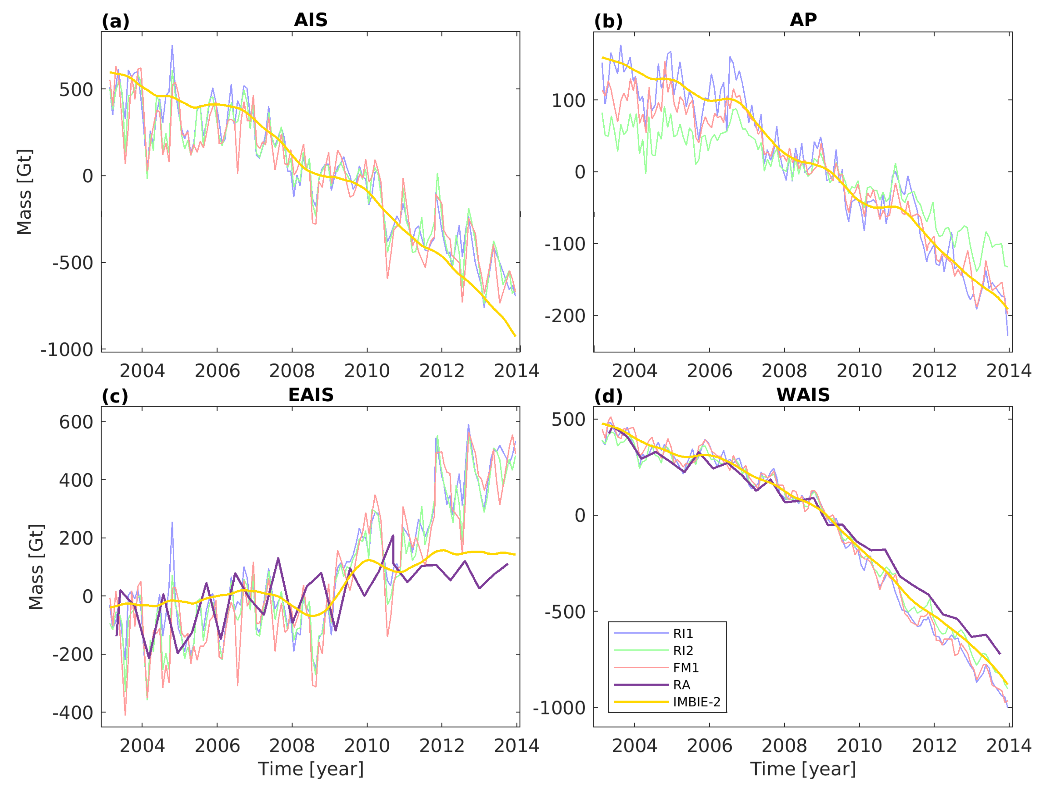
Figure 15c,d compares our GRACE mass change time series for EAIS and WAIS with those derived from RA [18]. Since the RA time series exhibit a temporal sampling of 140 days, less temporal variations can be revealed compared to GRACE. However, for WAIS RA confirms the general mass loss observed by GRACE, although the RA mass loss is slightly smaller. The most striking difference for EAIS is related to the accumulation events in 2009 and 2011, whose magnitude is clearly larger in the GRACE time series. After the 2011 event the data sets exhibit differing trends. These differences could be explained by the density mask used to convert RA-observed height changes into mass changes. This mask is constant in time and does not account for temporal changes in the firn densification process, which might be triggered by the accumulation events. Moreover, the change in the surface properties also has an impact on the radar signal penetration. Because of these limiting factors in RA analysis, RA time series are not suitable for a rigorous validation. It is impossible to attribute revealed differences to either RA or GRACE.

In addition, we also made use of the reconciled mass change time series from IMBIE-2 [19], which are a combination of results from different approaches (altimetry, gravimetry, input-output-method). These time series are available for AP, EAIS, WAIS as well as the entire AIS and are also shown in Figure 15. It is noteworthy that some participants, namely, RI1, FM1 and MC1, have contributed variants of their GRACE products to IMBIE-2 and those products are therefore included in the reconciled IMBIE-2 time series. Hence, it is not surprising that the IMBIE-2 time series show a temporal characteristic which lies between that of RA and that of GRACE, as revealed for EAIS and WAIS. For AIS, the mass loss evident in the IMBIE-2 is slightly larger than shown by our GRACE results. For AP, which is a challenging region for both GRACE and RA, the RA time series is in good agreement with RI1 and FM1, while larger differences are visible for RI2. In general, for larger basins and aggregations, time series provided by RI2 are in better agreement with the other GRACE products and with independent data as for smaller drainage basins.

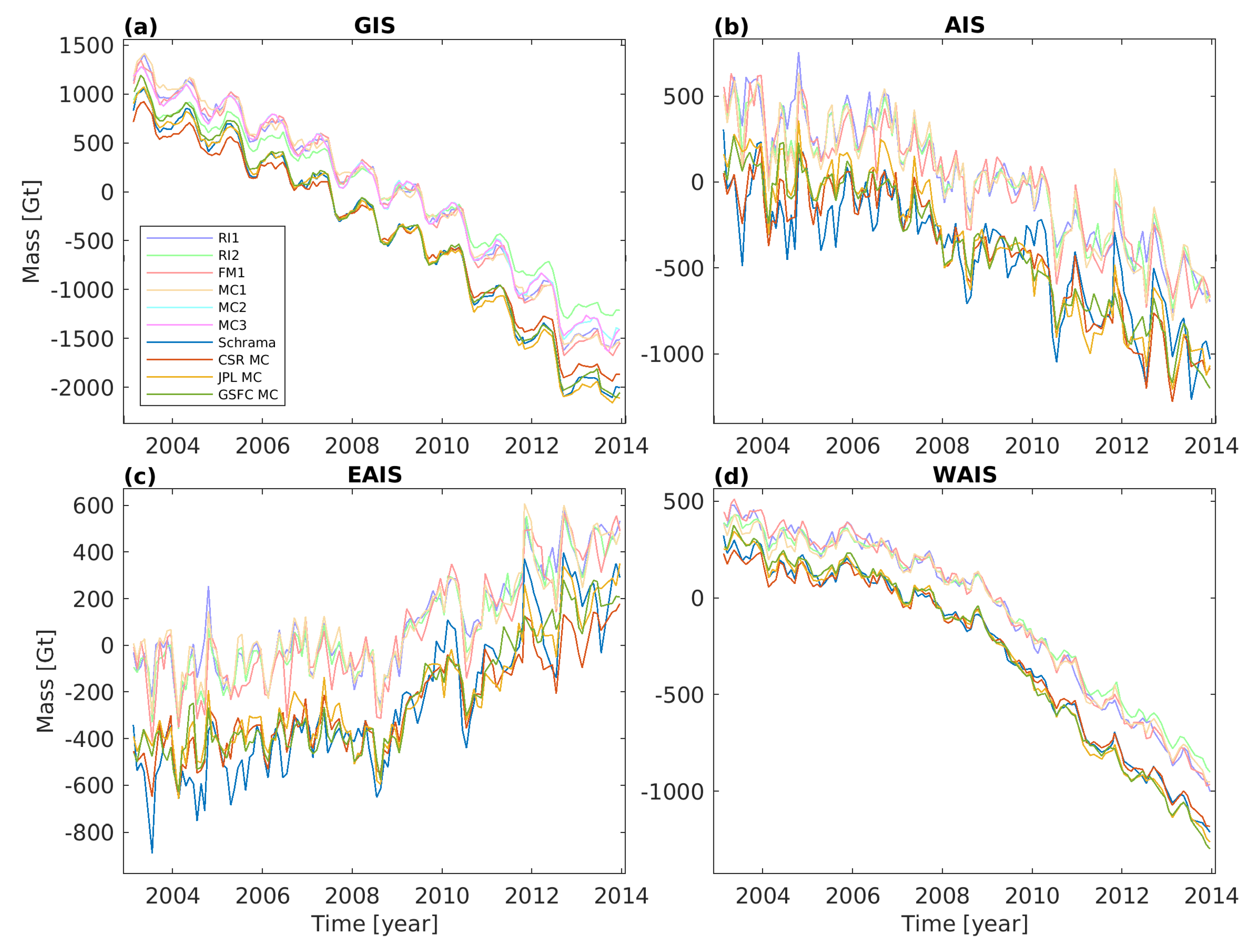
Figure 16 compares the mass change time series provided by the participants with alternative GRACE results (Section 2.4 (B)) for GIS, AIS, EAIS and WAIS. For the mascon solutions by CSR, JPL and GSFC, time series for all remaining drainage basins are depicted by Figures S1–S5, S14 and S15. Temporal variations and noise levels were derived in the same way as described in Section 2.4 (C) and (D), respectively, and are summarised in Tables S1–S4. The linear trend of the GIS time series by CSR MC (−258 Gt/yr) falls within the range of the trend estimates derived from our time series (−252 – −274 Gt/yr exluding RI2), whereas the mass loss rates of Schrama (283 Gt/yr), JPL MC (293 Gt/yr) and GSFC MC (291 Gt/yr) are larger. The smallest differences were found for the most norther basin GIS01, where our estimates vary from −24 to −28 Gt/yr and the three MC solutions exhibit trends between −25 and −30 Gt/yr. Differences between our trend estimates and the mean MC trend are shown in Figure S17a. We found a general good agreement for the estimated seasonal amplitudes. For the entire GIS and the majority of the basins, the noise level of RI1, FM1 and MC1 is larger than the average noise level of the MC solutions, while RI2 and MC2/MC3 exhibit a smaller or comparable noise level (Figure S17b).

The AIS mass loss inferred from the Schrama solution (92 Gt/yr) is lower than what we found for our solutions (99–108 Gt/yr). This is mainly because of a more pronounced mass gain for EAIS (82 Gt/yr) and is most likely related to the different GIA correction applied [56]. Just like for GIS, the MC solutions exhibit a stronger mass loss for the AIS than our solutions. The CSR MC mass loss (111 Gt/yr) is closest to our results, followed by GSFC MC (117 Gt/yr), while JPL MC (127 Gt/yr) reveals the largest mass loss. These differences originate from the WAIS, where especially JPL MC and GSFC MC observe a more negative mass change exceeding −145 Gt/yr. Generally speaking, the largest differences between the MC solutions and our solutions were found for basins exhibiting the largest mass changes (Figure S7a). In contrast, the seasonal amplitudes agree very well for the different solutions, except for the Schrama solution, which shows a significantly larger annual signal for EAIS. For nearly all AIS basins the noise level of the majority of our solutions (RI1, FM1, MC1) is larger than the RMS of the noise level derived from the three MC solutions (Figure S17b). For some basins, e.g., for AIS15 (Table S1) which is one of the smallest basins, the noise level of our solution significantly exceeds the MC noise level (in some cases by more than a factor of 2). Only RI2 exhibits a noise level which is comparable or even lower than that of the MC solutions.

Altogether, we found that the MC solutions reveal larger mass loss rates for the entire ice sheets and are beneficial with respect to the noise level of the mass change time series, especially when looking at smaller drainage basins (Figures S7 and S17). Unfortunately, we are not able to resolve the discrepancies in the linear trend. From the synthetic results provided by RI1, FM1 and MC1, we know that all solutions recover the mean annual mass changes comparably well. However, we have no possibility to draw a comparable conclusion for the MC solutions. The MC data sets are provided as global grids, from which the user can only extract the data for his region under investigation. There is no way to quantify signal leakage.

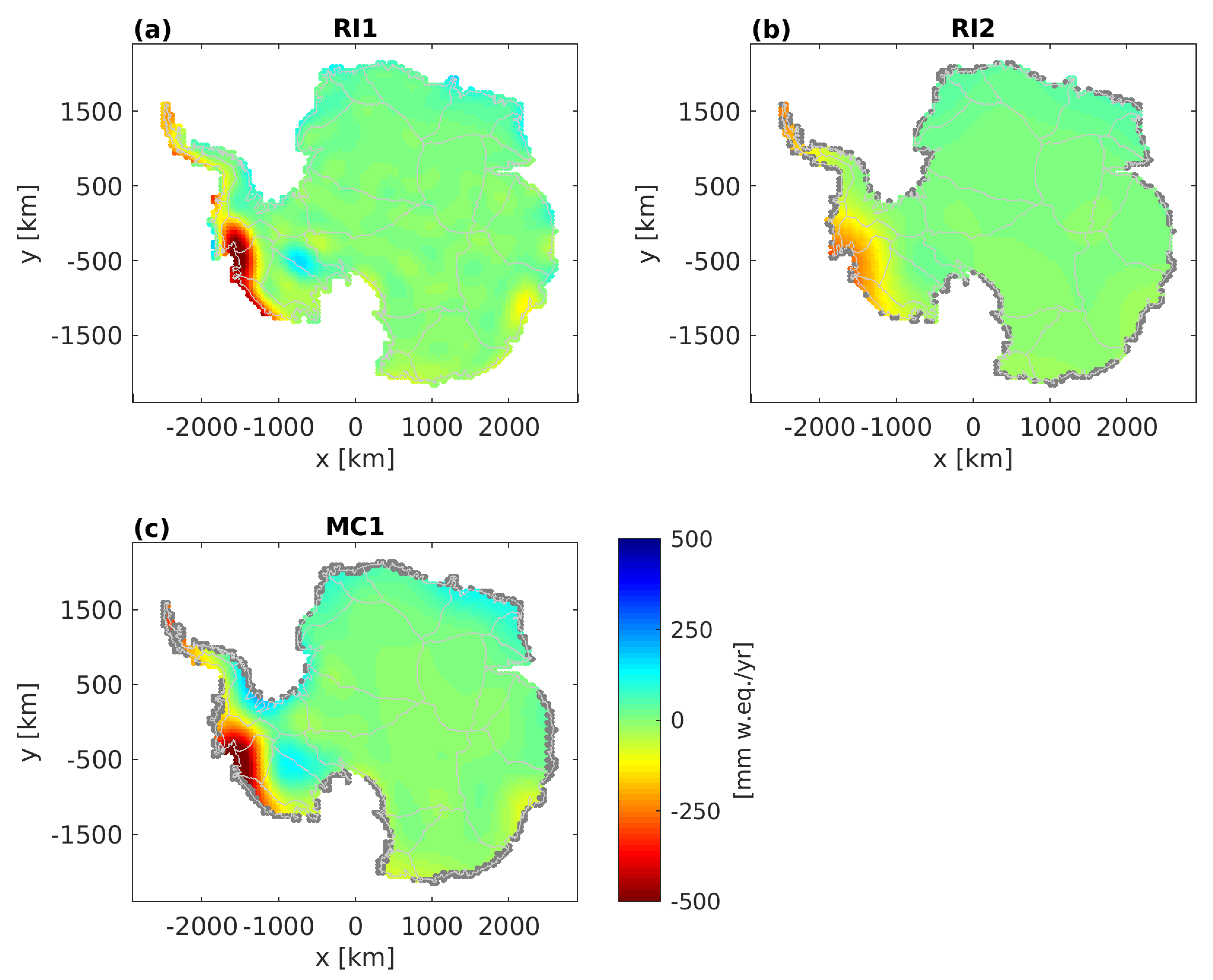
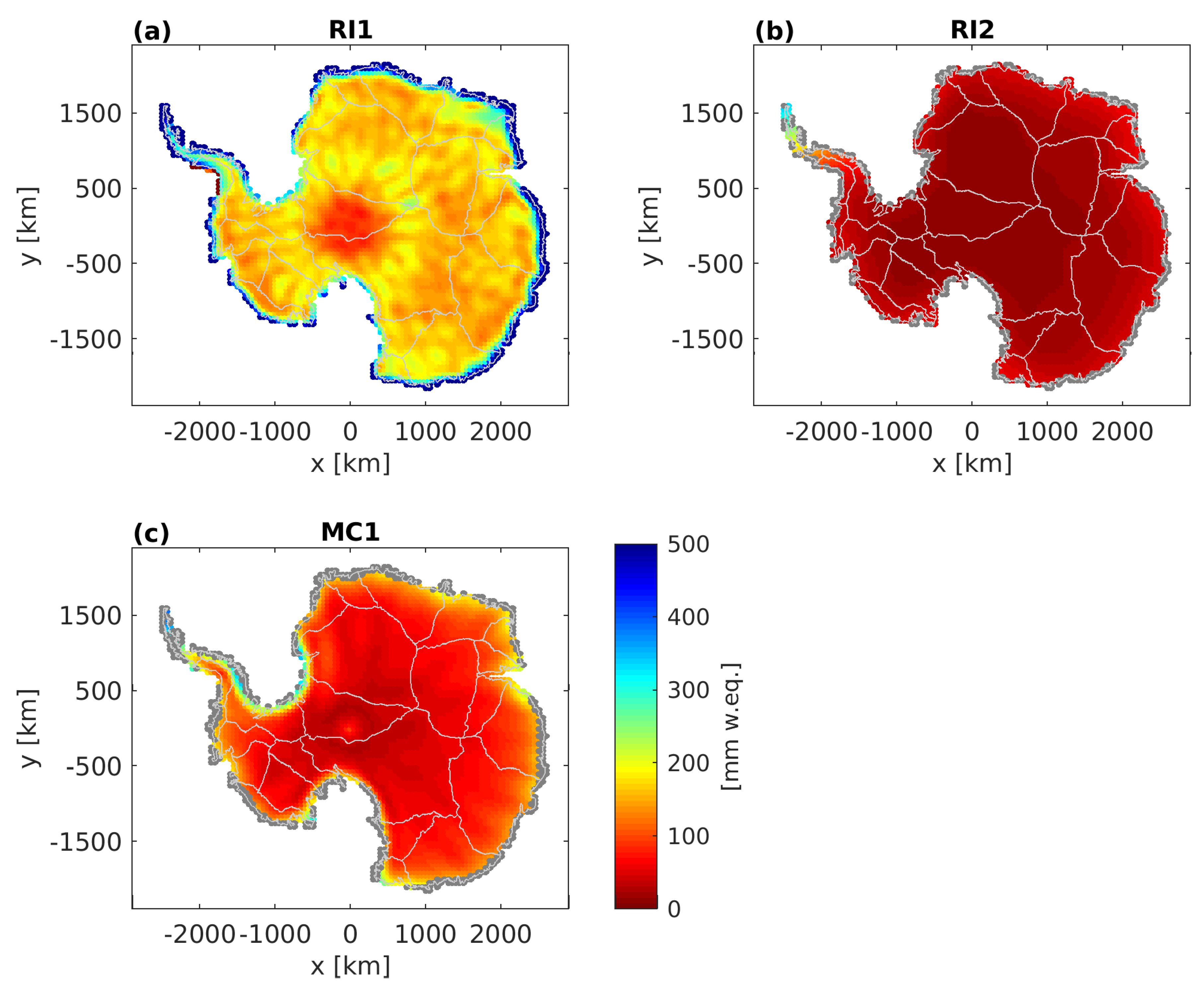
A comprehensive assessment was only possible for the results provided by RI1, FM1 and MC1. It could be shown that all three products are in general good agreement with respect to their noise level and the induced leakage errors, although the MC1 results exhibit slightly larger leakage errors for certain synthetic data sets. Nevertheless, from our analyses none of the three algorithms is clearly superior. Gridded products based on the FM1 algorithm have not been provided since the implied method does not involve sub-basin resolution. The generation of gridded products using FM1 does not seem to be straight forward. However, the algorithm to be selected has to be applicable for the production of both types of GMB products. It has also been shown that among the two methods suitable for the generation of gridded products, results by RI1 exhibit a somewhat larger noise level compared to MC1. A comparison between Figure 7 and Figure 8 suggests that the higher spatial resolution (i.e., smaller leakage) of RI1 was achieved at the expense of a higher noise level.

To summarise, since neither RI1 nor MC1 is clearly superior to the other, the final CCI GMB products are generated using various algorithms. The GIS_cci GMB products are available in two different versions based on both the MC1 algorithm and an updated version of the RI1 algorithm, while the AIS_cci GMB products are solely based on an update of RI1. This algorithm update was based on the findings of this study and reduced the noise level of RI1 by adjusting the weights given to the different conditions used for constructing the tailored sensitivity kernels. The finally generated AIS_cci and the GIS_cci GMB products are freely available through the projects’ websites (www.esa-icesheets-cci.org).

In addition, this study has clearly demonstrated that a fully rigorous assessment of GMB algorithms is only possible if a sufficient number of results, namely, complete sets including synthetic results, are available. This is the only way to comprehensively evaluate a product and to assess the algorithm’s ability to minimise both signal leakage and noise. Ideally, the synthetic data set could combine known geophysical signals in different subsystems of the Earth with GRACE-like errors, based on realistic assumptions for both instrument errors and background model errors. Satellite mission simulation studies [57] usually generate these kind of synthetic data in terms of an entire perennial GRACE-like time series instead of just a number of selected data sets like in our study. On the one hand side, this would allow one to derive leakage errors on different temporal scales (e.g., annual, inter-annual and long-term) instead of just month-to-month errors from selected epochs. On the other hand side, the algorithms’ ability to reduce leakage and to suppress GRACE errors could by tested in a single step. Consequently, any future inter-comparison exercise should involve time series of synthetic data which cover the entire Earth system and include realistic GRACE-like errors. One could even go one step further. After the algorithms have been evaluated using identical input data and background models for all participants, the algorithms could be applied to different input data (e.g., GRACE solutions, degree one and C${}_{2,0}$ time series, GIA model corrections). Performing such extensive experiments is a big effort but still urgently needed. We hope that this study could help to raise the awareness of this necessity and to encourage people to participate in upcoming inter-comparison exercises, e.g., in a possible continuation of IMBIE.